A New Wave of Hybrid Algorithms for Roots of Transcendental and Non-Linear Equations

Preprint

Article

A New Wave of Hybrid Algorithms for Roots of Transcendental and Non-Linear Equations

Altmetrics

Downloads

Views

Comments

Chaman Lal Sabharwal^*

This version is not peer-reviewed

Submitted:

26 December 2023

Posted:

28 December 2023

You are already at the latest version

Alerts

Abstract

Finding the roots of an equation is a fundamental problem in diverse fields. Optimization problem leads to non-linear equations for calculating the roots of the equation efficiently. Numerical iterative techniques are frequently applied when analytic solution is not available. Hybrid techniques to find roots of an equation is new to this fundamental problem. Recently, some attempts emerged to design hybrid algorithms for efficient solutions. A new heuristic algorithm is designed which is an intuitive approach to hybridization. In this paper, we implement two new algorithms: (1) a new BTsection algorithm blending the Bisection and Trisection algorithm, (2) a hybrid algorithm, that promises to be more efficient than the existing hybrid algorithms. The new hybrid algorithm is a blend of BTsection algorithm and Regula Falsi algorithm. The implementation results validate that the new algorithm, Hybrid4, surpasses the efficiency of existing hybrid algorithms Hybrid1, Hybrid2, and Hybrid3 algorithms. This paper contributes an essential hybrid algorithm to the repertoire of hybrid root finding algorithms.

Keywords:

Subject: Computer Science and Mathematics - Computational Mathematics

1. Introduction

Numerical iterative techniques are applied to find roots of an equation when analytic solution is not available [1,2,3,4]. Hybrid algorithm is a new concept to iterative solutions. Envisioning hybrid techniques to find roots of an equation is an inspiring technique to solve the fundamental problem in diverse fields. Recently, there have been some hybrid algorithms designing efficient solutions. Here we present a new hybrid algorithm which is a more intuitive and heuristic approach to hybridization.

Mostly optimization problems lead to solving non-linear equations for optimizing calculation of the value of a parameter, that is the root of the equation. We design and implement a new algorithm Hybrid4 that is more efficient hybrid of BTsection and False Position methods. The implementation results validate that the new algorithm surpasses the existing hybrid algorithms rooted on standalone Bisection and Trisection algorithms in conjunction with False Position and Newton Raphson algorithms. We designed and implemented an essential hybrid algorithm to the root finding algorithms.

First, why do we need another root finding algorithm? Even though the classical methods have been developed and used for decades, enhancements are progressively made to improve the performance of these methods [5]. There are several factors in determining the efficiency of an algorithm: accuracy, CPU time efficiency, and generality that it is works most of the time on all functions and domain intervals as expected. Accuracy may be measured in terms of number of decimal digits. For iterative methods, efficiency could mean the number of iterations to arrive at a solution coupled with CPU times, and computational complexity of iteration etc.

Finding the roots of an equation is a fundamental problem in diverse fields in physical and social sciences including Computer Science, Engineering (Biological, Civil, Electrical, Mechanical), and Social Sciences (Psychology, Economics, Businesses, Stock Analysis) etc. They look for the optimal solution to the recurring non-linear problems. The problems such as minimization, Target Shooting, Orbital Motion, Plenary Motion, Social Sciences, Financial Market Stock prediction analysis etc, lend themselves to finding roots of non-linear functional equations [6,7]. There is thorough study by Sapna and Mohan in the financial sector away from mathematics [8].

Thus, a root-finding algorithm implies solving an equation defined by a function that may be linear, non-linear or transcendental. Some root-finding algorithms do not guarantee that they will find a root. If such an algorithm does not find a root, that does not mean that a root does not exist. No single classical method outperforms another method on all functions [9]. A method may outperform other methods on one input and may produce inferior results on another input. Different methods have their own strengths/weaknesses.

There are classical root-finding algorithms: Bisection, False Position, Newton-Raphson, Secant, methods for finding the roots of an equation f(x) = 0. Every textbook on Numerical Techniques has details of these methods [1,2,3]. In the presence of classical methods, enhancements are progressively made to improve the performance of these methods [10,11,12].

Recently papers are making a headway on seeking better performing methods. In response, the better algorithms that are hybrid of classical methods Bisection, Trisection, with False Position, Newton Raphson methods been developed, namely Hybrid1 [10], Hybrid2 [11], and Hybrid3 [12]. Inspired by these three algorithms, we have crafted a new proficient algorithm, Hybrid4, that is a blend of BTsection and Regula Falsi algorithms. This blended algorithm is comparatively better than Hybrid1, Hybrid2, and Hybrid3 with respect to computational efficiency, solution accuracy (less error) and iteration count required to terminate within the specified error tolerance. This algorithm, Hybrid4, further optimizes these algorithms, first by blending Bisection and Trisection algorithms, then the resulting algorithm is blended with False Position method to evolve into Hybrid 4 algorithm hybridizing one step further by eliminating some of the computing time and increasing the efficiency of the algorithm.

The paper is organized as follows. Section II is brief description of classical methods Bisection, Regula Falsi, Newton-Raphson, Secant; their strengths and pitfalls. In addition, Trisection and new BTsection algorithms are included. Section III describes hybrid algorithms and a new algorithm, Hybrid4, that blends BTsection and False Position algorithms. Section IV presents experimental results simulating the performance of new algorithm Hybrid4 and validating it by comparing its performance with the previous hybrid algorithms. Section V is conclusion.

2. Related Background

The classical algorithms Bisection, False Position, Newton-Raphson, Secant methods are readily found in any text book in detail and iterated in most articles [1,2,3]. The classical algorithms, that are ubiquitous are available everywhere, These are iteration based methods. BIS-Bisection method compute a new approximation at the mid point of the interval, FP-FalsPosition obtains a new approximation by the secant line joining the endpoints of the function. NR- Newton Raphson derives new approximating by the tangent line at the iterated point on the function. All these algorithms are iterative for calculations of better approximations.

We will discuss the recent algorithms Trisection and BTsection. As Bisection method divides an interval into two equal parts, the Trisection algorithm subdivides the interval in three equal parts to get better estimate at the next iteration. BTsection is new algorithm that subdivides the interval adaptively into three parts: first Bisection into two, then the promising one half is adaptively trisected into parts to get better approximation, see algorithm in sectio3 [14].

Bisection algorithm states that “If f is continuous on a closed interval [a, b] and f is of opposite signs at the end points, i.e. f(a)f(b) < 0, then there is a root in the open interval (a, b).” Standard algorithm implementation expects that f(a)fb) < 0 to begin with. Because, f(a)f(b)=0 in the following, it will fail to proceed on this root finding problem: ” x²-x-2=0 on interval [2,4], or [0, 2], or [-2,-1] or [-3,-1]. A robust bisection algorithm first confirms that f(a)f(b) < 0 before proceeding to iterate. For example, for f(x) = (x-1)*(x-2)*(x-3) on the interval [1,3], the original version of algorithm will not start, but will succeed on [a,b] only when a, b are not 1, 2, 3.

In order to be successful on any interval including special cases, we reconsider the wording in this theorem and reformulate this theorem to include closed interval all the way. “If f is continuous on a closed interval [a, b] and f is not of same sign at the end points, i.e. f(a)f(b) <= 0, then there is a root in the closed interval [a, b].” The Bisection algorithm is generalized from “f(a)f(b) < 0” to “f(a)f(b ≤ 0” to include the interval boundary also in definition. For example, the equation x²-x-2=0 may show up in some applications with an interval like [2, 4], [0, 2]. Though, it may look simple but if f(a)f(b) = 0, then a or b must be a root, but we still want to know which one of a and b?

For approximate solutions using iterative methods, we have some idea about where the root may be. We should have initial guess as close to the location of root as far as possible. That is, we provide a start point or a guess or initial bracketing interval to the algorithm to iterate in search for the true approximate value of actual root, within some acceptable tolerance.

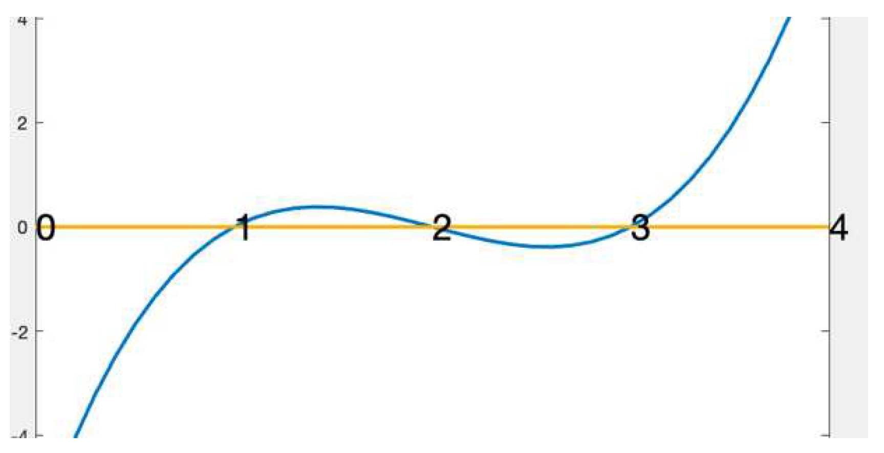
Figure 1. Modified version of Bisection on [1,3], succeeds in determining a root x=2 of (x-1)(x-2)(x-3)=0, in one iteration.

Since the Bisection, Regula Falsi, and Newton Raphson methods are readily available in the literature, their standalone derivations are skipped in this background section.

To enhance the performance of Bisection method, Bader et.al designed a Trisection method that supersedes Bisection method in finding an approximate root. Trisection method reduces the number of iterations performed, computation time, and error of approximation at a small cost on number of function computations. It inspired us to combine Bisection and Trisection algorithms to a BTsection algorithm at no additional compute cost and is at par with Trisection algorithm in computation CPU time, and error in approximate root, but BTsection requires fewer number of iterations, see examples in this section. These algorithms are blended with False Position and Newton-Raphson methods to construct hybrid algorithms. The effectiveness and efficacy of root approximation is measured by number of iterations in root calculation and the approximation accuracy of the root at the termination of algorithms. The heuristic metrics for measuring error, the number iterations and stopping criteria are elaborated here first.

Heuristics for comparing algorithms

2.1. Metric for Approximation Error Measurement

There are various ways to measure the error in the approximate root of an equations, f(x) = 0, at successive iterations to continue to a relatively more accurate approximation to the actual root. At iteration n, to determine r_n for which f(r_n)

≅

0, we proceed to analyze as follows.

The iterated root approximation error can be

RelativeRootError = |\frac{r_{n} - r_{n - 1}}{r_{n}}|

A b s o l u t e R o o t E r r o r = |r_{n} - r_{n - 1}|

Since a root can be zero, in order to avoid division by small numbers, it is preferable to use absolute error

|r_{n} - r_{n - 1}|

for convergence test. Another reason for this is that if r_n = 2^-n, then

|\frac{r_{n} - r_{n - 1}}{r_{n}}|

is always 1, it can never be less than 1, so the root-error tolerance test cannot be satisfied effectively, this test does not work. Since function value is expected to be zero at the root, an alternate cognitively more appealing error test is to use f(r_n) for error consideration instead of r_n. There are three versions for this concept, for comparison criteria, they are

R e l a t i v e V a l u e E r r o r = Q U O T E Q U O T E |\frac{f (r_{n}) - f (r_{n - 1})}{f (r_{n})}|

A b s o l u t e V l a u e E r r o r = |f (r_{n}) - f (r_{n - 1})|

T r u e V a l u e E r r o r = |f (r_{n})|

Since f(r_n) is to be close to zero near the root, in order to avoid divide by small numbers, we discard using

|\frac{f (r_{n}) - f (r_{n - 1})}{f (r_{n})}| .

Further, since

|f (r_{n}) - f (r_{n - 1})|

can be close to zero without |f(r_n)| being close to zero, we discard using

|f (r_{n}) - f (r_{n - 1})|

also in favor of using only

|f (r_{n})|

, trueValue error. For example, f(r_n)= (n-1)/n is such an example. We avoid using the first two criteria for this reason and exploit the last one,

|f (r_{n})|

Now we are left with two options

|r_{n} - r_{n - 1}|

and

|f (r_{n})|

to consider for error analysis. Again, r_n and r_n-1 can be closer to each other without f(r_n) being closer to zero. For example r_n = 1 +1/n, f(r_n) = r_n . Between the options

|r_{n} - r_{n - 1}|

and

|f (r_{n})|

, we find that

|f (r_{n})|

is the only reliable metric for analyzing the approximation error. Hence, we use,

|f (r_{n})|

, as the criteria for for comparing with tolerance error analysis for all the methods uniformly.

2.2. Metric for Iterations Stopping Criteria, Halting Condition

Stopping criteria plays a major role in simulations. The iteration termination (stopping) criteria for False Position method is different from Bisection method. Tradeoff between accuracy and efficiency is accuracy of the outcome. In order to obtain n significant digit accuracy, let

\in_{s}

be stopping error and let

\in_{a}

be the approximation error at any iteration. If

\in_{a}

\in_{s}

, the algorithm stops iterations. With

\in_{s}

= 5/10^n-1, we have n significant digit accuracy in the outcome [1]. The bisection algorithm is trivial [2], Trisection and BTsection algorithms are described in Section III.

Here we describe two enhancements to bisection algorithm. Trisection algorithm and BTsection [section III] algorithm, each algorithm has five comparison tests and reference to four function values. The BTsection algorithm uses the same amount of computation resources as Trisection algorithm.

But the number of iterations bn (Bisection), tn (Trisection), btn (BTsection) required by the Bisection, Trisection, and BTsection algorithms on [a, b] with stopping tolerance tol are

\frac{b - a}{2^{b n}} < t o l, \frac{b - a}{3^{t n}} < t o l, \frac{b - a}{6^{b n}} < t o l,

bn =log{(b-a)/tol} tn=(0.63) log{(b-a)/tol} btn= (0.39) log{(b-a)/tol}.

Trisection algorithm takes 37% fewer iterations than Bisection algorithm to converge within the desired tolerance.

BTesection algorithm takes 24% fewer iterations than Trisection algorithm to converge to the root within the desired tolerance. In addition, as observed below in both Trisection and BTsection algorithms, in each iteration, there is no change in the computation time: five comparison tests and references to four function values.

2.3. Criteria for Performance

This is an experimental science. The methods are numerical and iterative, not analytic solutions. A method may perform well in one case, and fail miserably in another case, see examples below. No one method outperforms all other methods all the time on all the intervals of definition [9,15]. We determine that the proposed algorithm performs better than the existing related algorithms.

There is no easy way to declare that an algorithm superior to other exiting algorithms. There are several factors that must be taken into consideration for distinguishing between the competing algorithms for a root finding problem.

Smart way is to represent new algorithm as to how the proposed algorithm differs from the other algorithms. To emphasize the new idea, it is also desirable that the new solution be applicable to a larger spectrum, devoid of incomplete domain. A simple customized example does not give a quantitative or qualitative view. We need to check the performance and applicability of the proposed approach in a broader scope. To comprehend this further, let us take the following example.

For example, the following problem shows that Trisection algorithm outperforms the other algorithms, see Table2 [Bader], [12], it gets the correct root in one iteration whereas other cited algorithms take more iterative steps, and more CPU time as well. One can infer from this example that the Trisection algorithm 2 and 3 work well and are superior to other algorithms. Of course, it is when input test function is x^2 - x – 2 and interval is [1, 4].

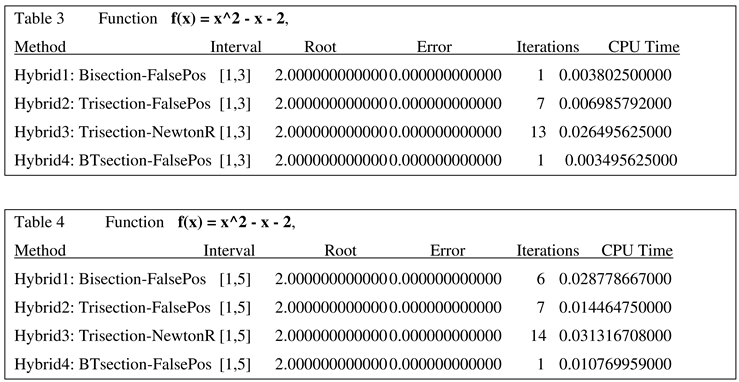
Now, consider the same function, and same four test algorithms. The initial input interval [1, 4] is changed to [1, 3] or [1, 5], the Table3 indicates that the inference from Table 2 does not hold good, the tables are turned, see Tables 3, 4. Here algorithm4 solves the same problem in one iteration and uses the lowest amount of CPU time. Again, from this example, it is unfair to declare that the algorithm 4 outperforms Algorithms 1, 2, 3. Considering Table 4, it gives a clue to inference. Even though algorithm4 doesn’t terminate in one iteration, it does terminate before the other algorithms.

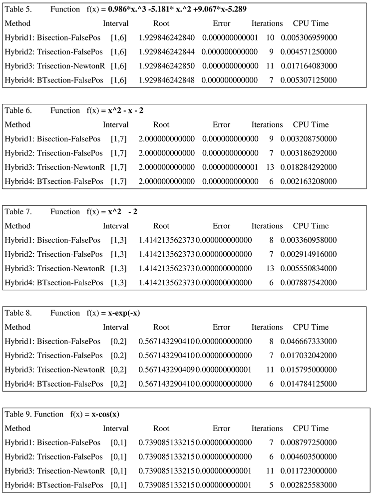
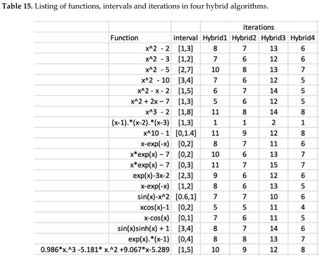
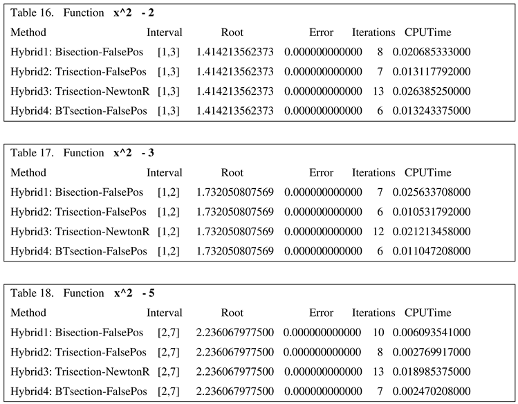
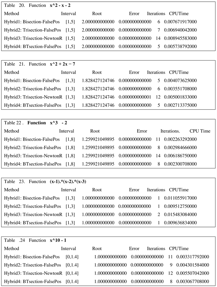
We have seen that in one case algorithms 2, 3 and in the other two cases algorithms 1, 4 come out ahead because they solve the problem in one iteration and use the lowest CPU time. The dilemma is is to determine which algorithm will work satisfactorily on the majority of cases, if not, all the cases. We have to consider not only this function but other functions as well; not one interval, but other related intervals as well. Let us first see the next examples in Tables 5,6,7,8,9 where none of these four algorithms succeed in finding the approximation in one iteration. We used different functions and different intervals for these examples in Tables 5,6,7,8,9. In all these examples, the algorithm 4 has the lowest number of iterations and lowest amount of CPU time. We have tested on number other examples as well to validate the same phenomena. The following examples use different functions and different initial intervals [1, 6], [1, 7], [1, 8], even [0, 1] as well to make a intuitive heuristic that algorithm 4 may be more efficient than the others. In all the ensuing examples in this paper, algorithm halting upperbound is 40 for iterations and upto 12 decimal digits for approximation in the acceptable root.

2.4. Algorithms

2.4.1. Bisection, Regula Falsi, Newton-Raphson algorithm

These algorithms are ubiquitous [1], [2], [3]]. We use Regula Falsi method for analysis of hybrid algorithms. There are multiple reasons for neglecting Newton Raphson from this analysis: (a) it requires that function be differentiable, (2) it depends heavily on the start point, (3) iterated approximations are not bracketed, (4) it fails if start point is not close to the root. Although False Position method is preferably used in hybrid algorithms, it does not fit well in the category of Bisection, Trisection and BTsection, we will first compare these algorithms.

2.4.2. Trisection Algorithm [11].

Bader extended bisection algorithm to trisection in order to create a better algorithm to hybridize it with false position algorithm. The algorithm is as follows.

Input: Function f(x), Initial approximations [a,b] and absolute error eps.

Output: Approximate root r, bracketing interval, and number of iterations k

for k=1 to n

p := (2*a +b)/3; q := (a +2*b)/3;

if |f(p)| < |f(q)|

r := p

else

r := q

endif;

if |f(r)| < eps

return r, a, b, k;

else if f(a)*f(p) < 0

b:=p;

else if f(p)*f(q) < 0

a:=p;

b:=q;

else

a:=q;

end if;

end for

2.4.3. BTsection Algorithm

In this paper, we adapted both Bisection and Trisection algorithms to craft a BTsection algorithm to hybridize, more heuristically, with False Position method [14]. BTsection algorithm incurs no more computational cost than the Trisection algorithm, but requires fewer iterations, in general, to reach an approximate solution. The algorithm is as follow.

Input: function f(x), Initial interval [a,b] and absolute error eps.

Output: Approximate root r, bracketing interval, and number of iterations k

for i=1:imax

bisection step

r=(a+b)/2;

if (f(a)*f(r)) < 0

b=r; r=(a+2*b)/3;

elseif (f(r)*f(b)) < 0

a=r; r=(2*a+b)/3;

else

return i, r, a, b

endif

trisection step

if (f(a)*f(r)) < 0

b=r;

elseif (f(r)*f(b)) < 0

a=r;

else

return i, r, a, b

endif

if |f(r)| < eps

return i,r,a,b ;

endif

endfor

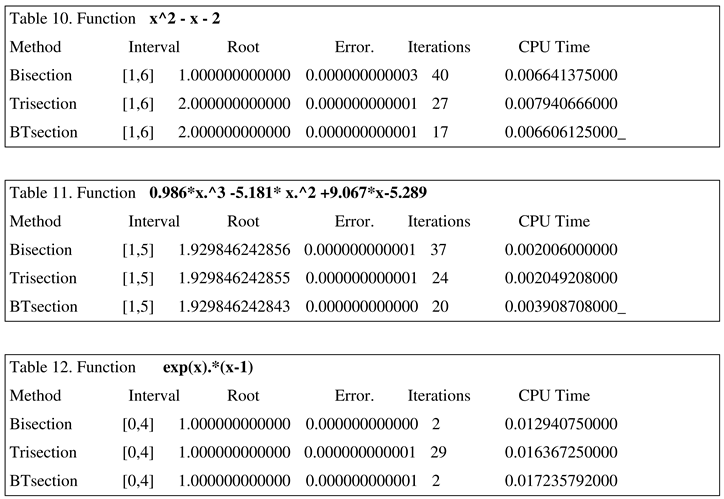
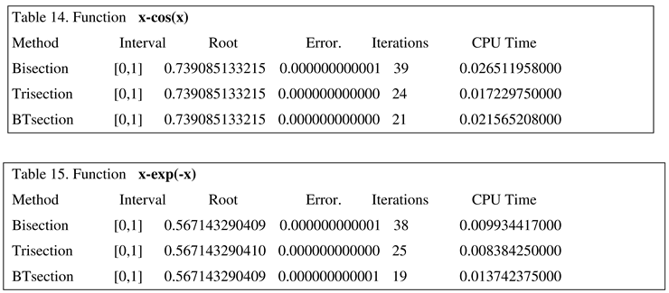
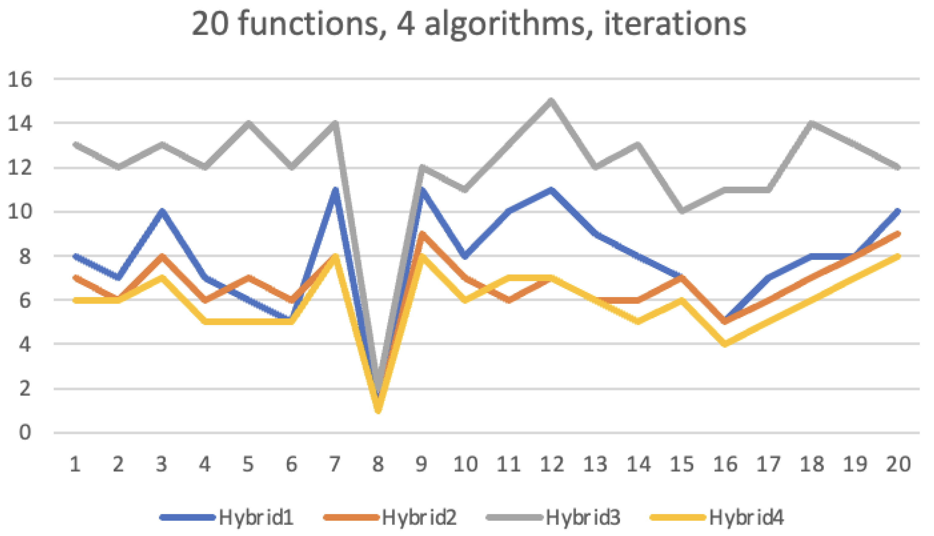
The Trisection algorithm and a new BTsection algorithm are conceptually equivalent in each iteration. From the following tables, it is clear that BTsection algorithm requires fewer iterations to converge. It shows that BTsection algorithm competes successfully with the other algorithms with respect to number of loop iterations, CPU time, and accuracy in approximation of the root. These benchmark functions appear in recent papers in the literature. See Tables 10–15 for comparing the performance of the sectioning algorithms. The functions and the interval of definition are generic of any algorithm. In all the ensuing examples in this paper, algorithm halting upperbound is 40 for iterations and upto 12 decimal digits for approximation in the acceptable root.

3. Hybrid Algorithms

Now we present recent hybrid algorithms and a new proposed hybrid algorithm. The existing hybrid algorithms have one thing in common. At each iteration, they compute the bracketing interval for each of the two hybridizing algorithms, and compute the interval common to the two algorithms to use at the next iteration. It incurs a computation step. Here in the new algorithm, there is no need to perform such computation because we can have the common interval readily available without performing this computation.

First we describe the original hybrid algorithm, namely, Hybrid1 based on classical Bisection and False Position algorithms. Since the classical algorithms can be found in any text book, those algorithms are not described here.

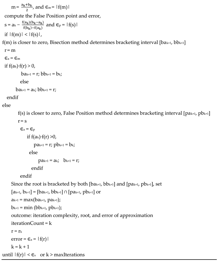
In Hybrid1 algorithm, at each iteration, more promising root between the Bisection and False Position approximate roots is selected, and common interval is computed for the next iteration. This curtails the unnecessary iterations in either method. It was succeeded by more efficient algorithms using Trisection method in place of Bisection algorithm: Hybrid2 and Hybrid3 [12]. These algorithms lead the way for us to discover more heuristics to design a new blended algorithm Hybrid4 which is more efficient than the previous three hybrid algorithms. All the four algorithms are described here for reference. For ease in readability, the prefixed variables use symbols: b for Bisection, p for False Position, t for Trisection, and bt for BTsection. The variables without prefix are algorithms local working variable.

Hybrid1: Bisection and False Position Algorithm [10]

Input: f , [a, b],

\in

maxIterations

Output: root r, k-number of iterations, error of approximation

\in

bracketing interval [a_k+1, b_k+1]

//initialize

k = 0; a₁ = a, b₁ = b

Initialize bounded interval for bisection and false position

pa_k+1=ba _k+1=a₁;pb_k+1=bb_k+1=b₁

repeat

pa_k+1=ba_k+1=a_k; pb_k+1=bb_k+1=b_k

compute the mid point the error

Hybrid2: Trisection and False Position Algorithm[11]

This function implements a blend of trisection and false position methods.

Input: The function f; the interval [a, b] where f(a)f(b) < 0 and the root lies in [a, b],

The absolute error (eps).

Output: The root (x), The value of f(x), Numbers of iterations (n), the interval [a, b] where the root lies in

n = 0; a1 := a; a2 := a; b1 := b, b2 := b

while true do

n := n + 1

xT1 := (b + 2*a)/3

xT2 := (2*b + a)/3

xF := a − (f(a)*(b − a))/(f(b) − f(a))

x := xT1

fx := fxT1

if |f(xT2)| < |f(x)|

x := xT2

if |f(xF)| < |f(x)|

x := xF

if |f(x)| <= eps

return x, f(x), n, a, b

if fa * f(xT1) < 0

b1 := xT1

else if f(xT1) * f(xT2) < 0

a1 := xT1

b1 := xT2

else

a1 := xT2

if fa*f(xF) < 0

b2 := xF;

else

a2 := xF;

a := max(a1, a2) ; b := min(b1, b2)

end (while)

Hybrid 3: Trisection and Newton-Raphson Algorithm

This algorithm is along the same lines as Hybrid 2, but with (1) instead of false position method, it uses Newton-Raphson algorithm which requires differentiability of the function, (2) improved iteration count and accuracy in the hybridization step: namely, the common interval in each iteration is computed by analyzing the five function values and then mapped to parameter values for the optimal interval.

The Algorithm is as follows.

Input: Function f(x), an Initial approximations x₀ and absolute error eps.

Output: Root x and number of iterations n

df(x):=f’(x); k:=0;

for k=1:n

p := (2*a + b)/3;

q := (a + 2*b)/3;

if |f(p)| < |f(q)|

then r := p - f(p)/df(p);

else r := q - f(q)/df(q);

end if;

if |f(r)| < eps

then

return r, k;

else

find fv:={f(a),f(b),f(r),f(p),f(q)};

a := xa where fv max -ve;

b := xb where fv min +ve

end if;

end.

Recall, in these three algorithms, there are two common steps to coordinate the two algorithms to hybridize. At each iteration, they determine (1) the promising approximation root out of the two roots (2) the common interval bracketing the approximate root. In Hybrid1 and Hybrid 2 algorithms, this simply reduces to intersection of two intervals so that common interval contains the approximate root. No function evaluation is involved in the search for common interval to contain the predicted approximate root. In the Hybrid3 algorithm, it searches among five function values used to determine two function values pertaining the common interval. From these two function values, the function parameters are determined to create the common bracketing interval.

New Hybrid Algorithm

Hybrid4 algorithm provides a more proficient approach to optimization: (1) BTsection algorithm is used instead of bisection or trisection, (2) it eliminates the computation of common interval required by the foregoing algorithms used to hybridize, There is no work needed to determine the better of the two roots. This leads to more efficiency for optimal root approximation and readily available common interval. It is based on common sense Occam’s razor principle [13], Figure 2. The Occam’s razor principle is a heuristic, not a proof. That is, when faced with competing choices, we use the simplest from what we have. It will be shown that Occam’s Razor Principle works quite well in this case.

Hybrid4.

This algorithm is a blend of BTsection and False Position methods to find iteration approximations with minimal effort.

Input a₀, b₀, r_o, eps, imax, f

Output k, a_k, b_k, r_k

for k=1:imax

BTsection iteration step determines

bta_k, btb_k-, btr_k- from bta_k-1, btb_k-1, btr_k-1

relable

bta_k, btb_k, btr_k to a_k, b_k, r_{k -}

False-position iteration step

input is a_k, b_k, r_k instead of old pa_k-1, pb_k-1, pr_k-1

false position iteration step determines

pa_k,pb_k, pr_k- from a_k, b_k, r_k instead of from old pa_k-1, pb_k-1, pr_k-1

This makes [pa_k,pb_k] as the common interval [a_k, b_k] without any computation.

The use of a_k, b_k, r_k instead of old pa_k-1, pb_k-1, pr_k-1, makes this step more optimal for next approximation

if f(pr_k)<eps

return k, pa_k,pb_k, pr_k

end

relabel pa_k,pb_k, pr_k to qa_k, qb_k-, qr_k-

endFor

Summarizing the foregoing algorithms, succinctly the iteration step in the algorithms are:

Hybrid1

[ba_k,bb_k,br_k]= Bisection(a_k-1, b_k-1, r_k-1,f)

[pa_k,pb_k,pr_k]=FalsePosition(a_k-1,b_k-1, r_k-1,f)

The results of hybridization step are:

r_k is better of br_k pr_k,

[a_k,b_k] is common to [ba_k,bb_k], [pa_k,pb_k],

r_k belongs to [a_k,b_k]

Hybrid 2

[ta_k,tb_k,tr_k]=Trisection(a_k-1,b_k-1, r_k-1,f)

[pa_k,pb_k,pr_k]=FalsePosition(a_k-1,b_k-1, r_k-1,f)

The outcomes of hybridization are:

r_k is better of tr_k pr_k,

[a_k,b_k] is common to [ta_k,tb_k], [pa_k,pb_k],

r_k belongs to [a_k,b_k]

Hybrid3

[ta_k,tb_k,tr_k]=Trisection(a_k-1,b_k-1, r_k-1,f)

[na_k,nb_k,nr_k]=NewtonRaphson(a_k-1,b_k-1, r_k-1,f)

The upshot of hybridization is:

r_k as better of tr_k nr_k,

[a_k,b_k] is common from [ba_k,bb_k], [pa_k,pb_k] and nr_k by analyzing { f(ba_k), f(bb_k), f(na_k),f(nb_k), f(nr_k})}then finding from {{ ba_k,bb_k,pa_k,pb_k, nr_k}}.

r_k belongs to [a_k,b_k]

Hybrid4

[a,b,r]=BTsection(a_k-1,b_k-1, r_k-1,f)

[pa_k,pb_k,pr_k]=FalsePosition(a,b,r,f)

The conclusion of hybridization is: there is no need to do any work calculation: [a_k,b_k] is the same interval [pa_k,pb_k] containing r_k is the same as pr_k, the desired root. This algorithm is optimal in the number of iterations and the accuracy in approximate root.

4. Discussion

Many researchers focused their attention toward using such methods to solve their problems. The roots are calculated iteratively, along with the number of iterations within a specified tolerance. In this section, all the existing hybrid methods are compared. Error analysis is performed. It is validated here that Hybrid4 algorithm preferable than the existing algorithms Hybrid1, Hybrid2, and Hybrid3.

4.1. Empirical Evidence Testing.

We have tested our new algorithm Hybrid4 with other hybrid algorithms on diverse examples of functions found in articles in the literature to validate that new algorithm outperforms the other three hybrid algorithms.

4.2. Experiments in Matlab

Moazzam used Microsoft visual C++ to find roots, we used Matlab R2022A 64 bit (maci64) on MacBook Pro MacOS Sonoma 14.1.1 16 GB Apple M1Pro . Along with numerous different functions and varying intervals, we use the same frequently cited functions. Overall we have validated that the new algorithm performs better than all the hybrid algorithms. These tests indicate that hybrid with false position algorithm is still preferable to hybridization with Newton-Raphson possibly because the NR method requires that the function be differentiable.

For all these Tables 16–34, the functions are frequently occuring in the literature. For all the functions the upperbound on the number of iterations is 40 and acceptable approximation error bound is 10^-12 . These tables are for comparision of four algorithms number of iterations, CPU compute time, accuracy of the solution.

Frequently used twenty functions are compared for iterations efficiency. These functions are listed in the table. This table lists functions used in the simulations. Columns represent the functions, the interval of function’s domains, the number of iterations required by each of four algorithm to reach an approximate root within tolerance. Figure 3 is a visual representation of the table.

In the chart below, functions are along x-axis, number of iterations along y-axis, legend color indicates algorithms 1,2,3,4: Hybrid1 is series1 (blue) Hybrid2 is series2(magenta), Hybrid3 is serie3(gray), Hybrid4 is series 4 (yellow). Four algorithms are in the body of the chart.

The tables 16–34 depict the Matlab numerical outputs of the simulation on 20 functions.

V. Conclusion

We have designed and implemented a new algorithm Hybrid4, an efficient algorithm hybrid of BTsection and Regula Falsi methods. The algorithm was implemented in Matlab R2022A 64 bit (maci64) on MacBook Pro MacOS Sonoma 14.1.1 16 GB Apple M1Pro. The implementation tests Tables 15–34 and numerical and visual iteration count graph indicate that Hybrid4 outperforms the Hybrid1,Hybrid2, and Hybrid3 algorithms. The experiments on numerous datasets used in the literature validate that the new algorithm Hybrid4 is effective both conceptually and computationally. This algorithm is applicable to both differentiable and non-differentiable functions. This paper provides an essential algorithm for the practitioners and contribution to the repertoire of hybrid algorithms.

References

Steven C Chapra and Raymond P Canale, Numerical Methods for Engineers, 7th Edition, McGraw-Hill Publishers, 2015.
John H. Mathews and Kurtis K. Fink Numerical Methods Using Matlab, 4th Edition, 2004 ISBN: 0-13-065248-2 Prentice-Hall Inc. Upper Saddle River, New Jersey, USA.
J. F. Traub: Iterative Methods for the Solution of Equations, Chelsea Publishing company, New York, NY, USA, 1982.
Douglas Wilhelm Harder, https://ece.uwaterloo.ca/~dwharder/NumericalAnalysis/10RootFinding/falseposition/, accessed Jun 2019.
5. Ehiwario, J.C., Aghamie, S.O.; Comparative Study of Bisection, Newton-Raphson and Secant Methods of Root- Finding Problems; IOSR Journal of Engineering (IOSRJEN) www.iosrjen.org; ISSN (e): 2250-3021, ISSN (p): 2278-8719; Vol. 04, Issue 04 (April. 2014), ||V1|| PP 01-07.
Donna Calhoun https://math.boisestate.edu/~calhoun/teaching/matlab-tutorials/lab_16/html/lab_16.html accessed December 2023.
C. Thinzar, and N. Aye, "Detection the storm movement by sub pixel registration approach of Newton Raphson method" International Journal of e Education, e Business, e Management and e Learning, Vol. 4, No. 1, 2014.
S. Sapna, Biju R. Mohan, Comparative Analysis of Root Finding Algorithms for Implied Volatility Estimation of Ethereum Options, Computational Economics, https://doi.org/10.1007/s10614-023-10446-8, springer, August, 2023, pp.1-37. [CrossRef]
G. Moazzam, A. Chakraborty, A. Bhuiyan: A robust method for solving transcendental equations. Int. J. Comput. Sci., 9 (2012), 413–419.
Sabharwal, C. L. (2019). Blended root finding algorithm outperforms bisection and regula falsi algorithms. Mathematics, 7(11), 1118. [CrossRef]
Badr, E., Almotairi, S., & Ghamry, A. E. (2021). A comparative study among new hybrid root finding algorithms and traditional methods. Mathematics, 9(11), 1306. [CrossRef]
Srinivasarao, Thota A Blended Root-Finding Algorithm for Solving Transcendental Equations SNAPP, International Journal of Applied and Computational Mathematics, https://doi.org/10.21203/rs.3.rs-2956091/v1, May 2023, pp.1-9. [CrossRef]
Occam’Razor: https://conceptually.org/concepts/occams-razor, accessed December 2023.
G.E. Collins and A.G. Akritas Trisection using Bisection, https://www.lamath.org/journal/Vol1/trisection_using_bisection.pdf, 1976.
Srivastava, R.B and Srivastava, S (2011), Comparison of Numerical Rate of Convergence of Bisection, Newton and Secant Methods. Journal of Chemical, Biological and Physical Sciences.Vol 2(1) pp 472-479, 2011.
Wikipedia https://en.wikipedia.org/wiki/False_position_method#Two_historical_types accessed December 2023.

Figure 2. https://conceptually.org/concepts/occams-razor.

Figure 3. Comparing iterations in twenty functions by four algorithms.

Disclaimer/Publisher’s Note: The statements, opinions and data contained in all publications are solely those of the individual author(s) and contributor(s) and not of MDPI and/or the editor(s). MDPI and/or the editor(s) disclaim responsibility for any injury to people or property resulting from any ideas, methods, instructions or products referred to in the content.

© 2023 by the authors. Licensee MDPI, Basel, Switzerland. This article is an open access article distributed under the terms and conditions of the Creative Commons Attribution (CC BY) license (http://creativecommons.org/licenses/by/4.0/).

Copyright: This open access article is published under a Creative Commons CC BY 4.0 license, which permit the free download, distribution, and reuse, provided that the author and preprint are cited in any reuse.

MDPI Initiatives

Important Links

Choose an area of interest and we will send you notifications of new preprints at your preferred frequency.

Disclaimer

A New Wave of Hybrid Algorithms for Roots of Transcendental and Non-Linear Equations

Abstract

1. Introduction

2. Related Background

2.1. Metric for Approximation Error Measurement

2.2. Metric for Iterations Stopping Criteria, Halting Condition

2.3. Criteria for Performance

2.4. Algorithms

2.4.1. Bisection, Regula Falsi, Newton-Raphson algorithm

2.4.2. Trisection Algorithm [11].

2.4.3. BTsection Algorithm

3. Hybrid Algorithms

4. Discussion

4.1. Empirical Evidence Testing.

4.2. Experiments in Matlab

References

MDPI Initiatives

Important Links

Subscribe