A Method for Developing Fragility Curves for Soil Liquefaction Consistent with the Seismic Hazard Using Monte Carlo Simulation

Preprint

Article

A Method for Developing Fragility Curves for Soil Liquefaction Consistent with the Seismic Hazard Using Monte Carlo Simulation

This version is not peer-reviewed.

This version is not peer-reviewed.

Altmetrics

Downloads

Views

Comments

Submitted:

28 December 2023

Posted:

28 December 2023

You are already at the latest version

A peer-reviewed article of this preprint also exists.

Abstract

The aim of this study is to present a method for developing fragility curves for soil liquefaction that are consistent with the seismic hazard using Monte Carlo simulation. This method can account for all the uncertainties and variabilities of the input parameters. The seismic parameters of earthquake magnitude (M) and the associated peak ground acceleration (PGA) are considered together for the liquefaction assessment. The liquefaction potential and damages obtained by this method are more realistic. A case study is performed using data from a sand-boil site in Yuanlin, Changhua county, where liquefaction occurred during the Chi-Chi earthquake in Taiwan in 1999. The results show that the liquefaction potential index, IL, the post-liquefaction settlement, St, and the liquefaction probability index, PW, are all suitable parameters for evaluating the liquefaction damages. The fragility curves for soil liquefaction developed by this method can support the performance-based earthquake engineering (PBEE) approach, provide guidance for liquefaction evaluation to the ‘Taiwan Earthquake Loss Estimation System’-TELES, and serve as a basis for scenario simulation and an earthquake early warning system for liquefaction damages.

Keywords:

Subject:

Engineering - Civil Engineering

1. Introduction

Taiwan lies on the ring of fire around the Pacific Ocean and has experienced many devastating earthquakes in its past. Earthquakes are unavoidable and their impact has to be taken seriously. One of the common types of ground failure during an earthquake is soil liquefaction [1,2,3]. Therefore, assessing liquefaction is a crucial issue for earthquake disaster management. To minimize seismic losses from earthquakes, earthquake disaster scenarios and earthquake early warning systems are important for updating the seismic code and for ensuring seismic safety and risk reduction [3]. Hence, developing fragility curves for soil liquefaction is a key part of these goals. In this study, we propose a method to construct hazard-consistent fragility curves for soil liquefaction using Monte Carlo simulation. We apply this method to the data from the sand-boil site in Yuanlin town of Changhua county that was affected by the Chi-Chi earthquake in Taiwan in 1999. The results can not only match the development trends of PBEE, but also provide guidance for the simulation of liquefaction damage scenarios in the ‘Taiwan Earthquake Loss Estimation System’-TELES [4,5].

2. Liquefaction Fragility

2.1. Fragility Assessment Method

If the damage index of liquefaction is denoted by the random variable X, the probability that X exceeds a specified value of x in t years can be evaluated by the total probability theorem to incorporate the contribution from all values of intensity measure (IM) of earthquake (e.g., peak ground acceleration, PGA) as:

P {[X > x]}_{t} = \int P [X > x | I M = a] [- \frac{d H_{t} (a)}{d a}] d a

(1)

where

H_{t} (a) = P {[I M > a]}_{t}

(2)

H_t(a) is the hazard curve that describes the probability of exceeding a in t (for example, 50) years, which can be constructed from probabilistic models of the source, path, and site based on available regional seismicity information.

The item of

P [X > x | I M = a]

in Equation (1) is now defined as the seismic fragility of liquefaction:

F (x; a) = P [X > x | I M = a]

(3)

If three types of damage state (DS) are assumed: D₃ (light to no damage), D₂ (medium damage), and D₁ (extreme damage), the probabilities for these three damage states of liquefaction of a soil layer subjected to an earthquake are defined as:

P [D S = D_{3} | I M = a] = F (x_{3}; a)

(4a)

P [D S = D_{2} | I M = a] = F (x_{2}; a) - F (x_{3}; a)

(4b)

P [D S = D_{1} | I M = a] = 1 - P [D S = D_{3} | I M = a] - P [D S = D_{2} | I M = a]

(4c)

2.2. Damage Evaluation of Soil Liquefaction

In engineering practice, concerns are not only focused on the liquefaction potential at a specific depth, there is also a need to predict the overall potential of liquefaction to cause foundation damages. In this study, three liquefaction damage indices are adopted. It is liquefaction potential index (I_L), liquefaction-induced settlement (S_t), and liquefaction probability index (P_W). Each index and associated damage states are described in the following.

Iwasaki et al. (1982)[6] proposed a liquefaction potential index (I_L) using the factor of safety (FS) against liquefaction and the depth weighting factor (W) to quantify the severity of the degree of liquefaction at depths ranging from 0 to 20m beneath the ground as below:

I_{L} = \int_{0}^{20} F \cdot W (z) d z

(5)

or in discrete form:

I_{L} = \sum_{i = 1}^{n} F_{i} \times W_{i} \times H_{i}

(6)

where

F_{i} = {\begin{cases} 1 - F S_{i} f o r 0 \leq F S_{i} \leq 1 \\ 0 f o r F S_{i} > 1 \end{cases}

(7)

and

W_{i} = 10 - 0.5 z_{i}

(8)

In which z is the depth of the soil in metres; H is the thickness of the soil layer considered. The severity of liquefaction was classified into four classes called ‘‘very low,’’ ‘‘low,’’ ‘‘high’’ and ‘‘very high’’, depending on the value of I_L shown in Table 1, proposed by Iwasaki et al. (1982) [6].

The second damage index used in this study is liquefaction-induced settlement, which could result in collapse or partial collapse of a structure, especially if there is significant differential settlement between adjacent structural elements. The total settlement, S_t, for sandy soil is given by:

S_{t} = \sum_{i = 1}^{n} ε_{v i} H_{i}

(9)

where H_i = thickness of layer i ; ε_vi = volumetric strain of layer i; and n = number of soil layers.

Ishihara and Yoshimine (1992)[7] developed a practical method by correlating volumetric strain with relative density and associated penetration resistances (SPT-N value and CPT tip resistance) and the factor of safety (FS) of the sand against the state of liquefaction. It can be used to compute the settlements in Equation (9). The relationship between the extent of the damage and the approximate settlements is shown in Table 2.

When evaluating I_L and S_t in Equations (6) and (9), the simplified method [8,9] is used first to calculate the factor of safety against liquefaction, denoted by FS_Seed. And then Equation (10) is adopted to convert FS_Seed to FS (as mentioned above) based on the research by Huang [10] to determine the factor of safety in the case of equal probability of liquefaction.

FS = 1.1417 FS_Seed^0.5433

(10)

The third damage index used in this study is the liquefaction probability index (P_W). Because the probability of liquefaction, P_L_iq, is the information required to make risk-based design decisions, the following expression of P_L_iq derived by Huang (2008)[11] using logistic regression is used to evaluate the potential for liquefaction in this study:

P_{L i q} = \frac{1}{1 + \exp {- [10.097 - 0.245 {(N_{1})}_{60 c s} + 3.757 \ln (C S R N)]}}

(11)

where

C S R N = C S R / M S F = 0.65 \cdot (\frac{a_{\max}}{g}) (\frac{σ_{v 0}}{{σ^{'}}_{v 0}}) r_{d} / {(\frac{M_{w}}{7.5})}^{- 2.56}

(12)

in which

{(N_{1})}_{60 c s}

is the clean sand equivalence of the corrected SPT blow count defined in Youd et al. (2001) [9]. CSRN is the normalized cyclic stress ratio (CSR) shown in Equation (12) where MSF = magnitude scaling factor; a_max= peak horizontal acceleration of ground surface; g = acceleration due to gravity; σ_v₀ = total vertical stress in question; σ′_v₀ = effective vertical stress at the same depth;

r_{d}

= stress reduction factor defined by Youd et al. (2001) [9]; and

M_{w}

= moment magnitude.

To represent the overall liquefaction potential in the upper 20 m of the site profile, the liquefaction probability index, P_W, is defined below [11]:

P_{W} = \frac{\int_{0}^{20} P_{L i q} (z) W (z) d z}{\int_{0}^{20} W (z) d z}

(13)

where

P_{L i q} (z)

is the value of P_Liq at depth of z, and the weighting function W(z)=10-0.5z.

The liquefaction damage states are classified into three classes: ‘‘minor,’’ ‘‘moderate,’’ and ‘‘heavy’’, according to the value of P_W shown in Table 3, proposed by Huang [11].

3. Hazard-Consistent Fragility Curves of Soil Liquefaction

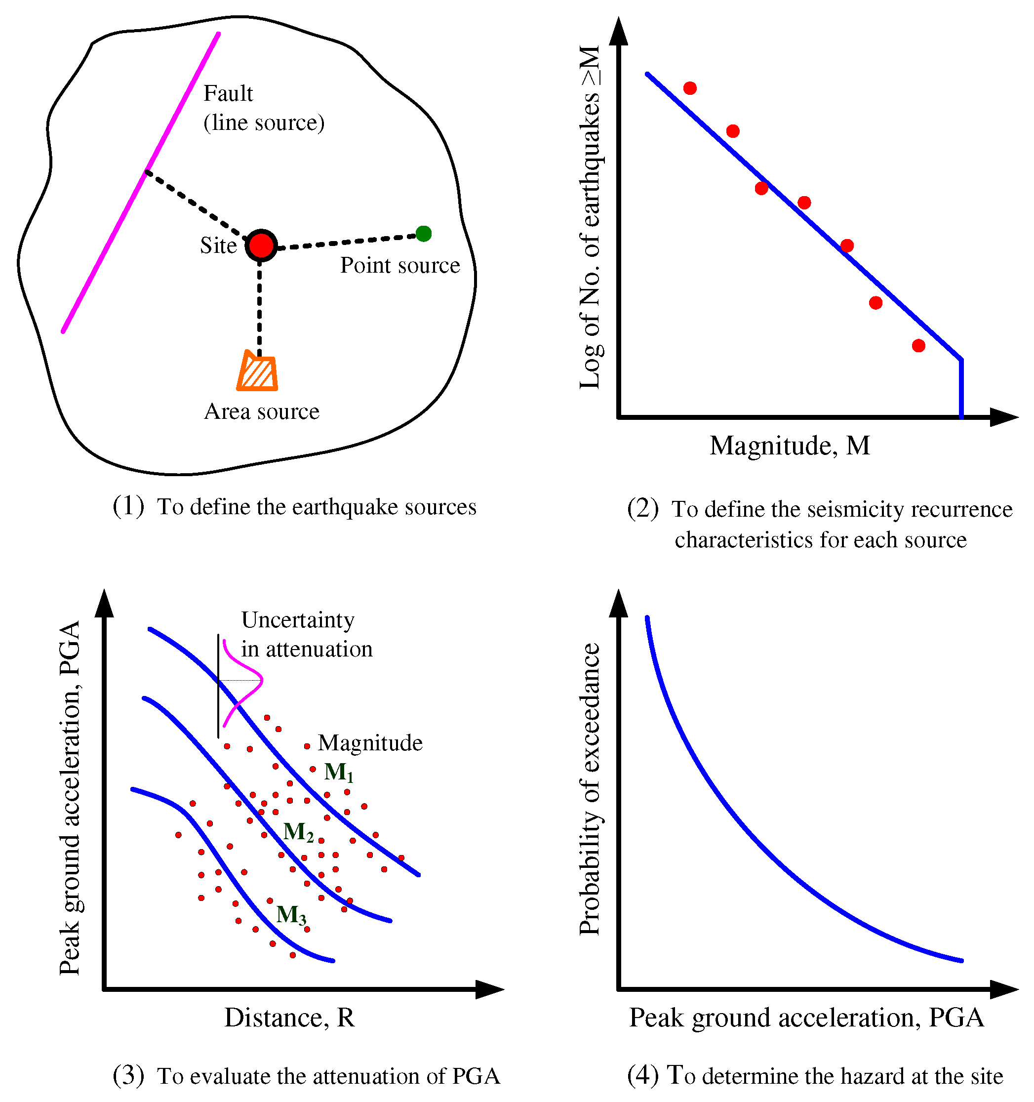
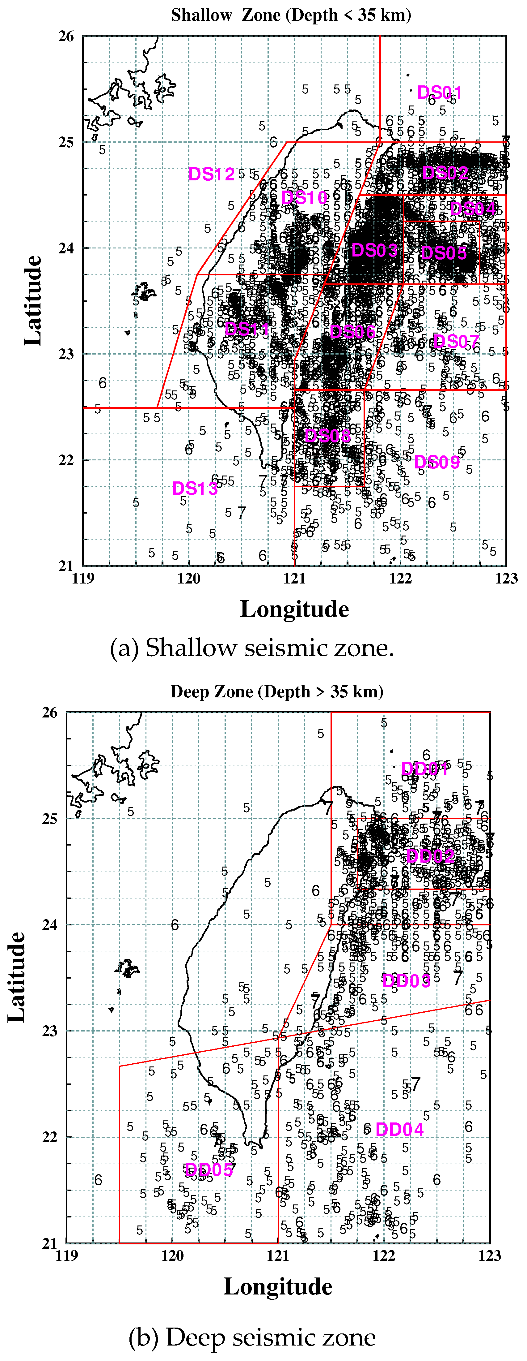
To evaluate the liquefaction damage of soil, this study uses the Monte Carlo simulation to generate the combination of earthquake magnitude (M) and peak ground acceleration (PGA), which are the seismic parameters for the assessment. The simulation methods and the seismic source database are consistent with those used in probabilistic seismic hazard analysis, so the resulting parameters are also hazard-consistent. Moreover, the hazard-consistency is maintained in the fragility curves of the soil liquefaction analysis.

3.1. Procedures for Seismic Hazard Analysis

Probabilistic seismic hazards can be divided into four steps [12], as shown in Figure 1.

The first step is to identify the earthquake sources. As Figure 2 illustrates, this study models the sources in the deep seismic zone (hypocentral depth > 35 km) as point sources [13]. On the other hand, in the shallow seismic zone (hypocentral depth < 35 km), the sources are modelled as area sources or line sources (such as active faults) [14].

The next step is to describe how often and how strongly each source produces earthquakes, or, in other words, the relationship between the frequency and the magnitude of seismic events. A maximum possible earthquake is selected for each source.

The third step is to assess the impact of the earthquake. To calculate how the peak ground acceleration (PGA) decreases with the magnitude (M) and the distance from the site to the source (R), this study uses the Campell's formula [15]:

P G A_{R} = f (M, R) = b_{1} e^{b_{2} M} {[R + b_{4} \exp (b_{5} M)]}^{- b_{3}}

(14)

σ_lnE = 0.68

(15)

where

P G A_{R}

is the horizontal PGA value for hard site conditions; b₁~b₅ are regression coefficients with values of b₁＝0.00369, b₂＝1.75377, b₃＝2.05644, b₄＝0.12220 and b₅＝0.78315, respectively [16]. σ_lnE is the standard deviation of the natural logarithm of the model error.

The next step is to estimate the site's seismic hazard, which means calculating how likely it is that different levels of ground shaking will occur at the site in a given year. The seismic hazard analysis is based on the assumption that earthquakes follow a stationary Poisson process, which means that they occur randomly and independently over time.

If go through the above four steps, the annual probability of peak ground acceleration, PGA_R, exceeding a value a can be expressed as [14]:

P {[P G A_{R} > a]}_{1 y e a r} = 1 - \exp {- \sum_{i = 1}^{n} P [P G A_{R} > a | E_{i}] \cdot v_{i}}

(1)

where n is the number of potential seismic sources in the region of the site;

E_{i}

is the event that the earthquake with M ≥ M₀ occurs in source i ;

v_{i}

is the annual average occurrence rate of earthquakes with M ≥ M₀ in source i; and M₀ is the smallest magnitude of concern to engineering.

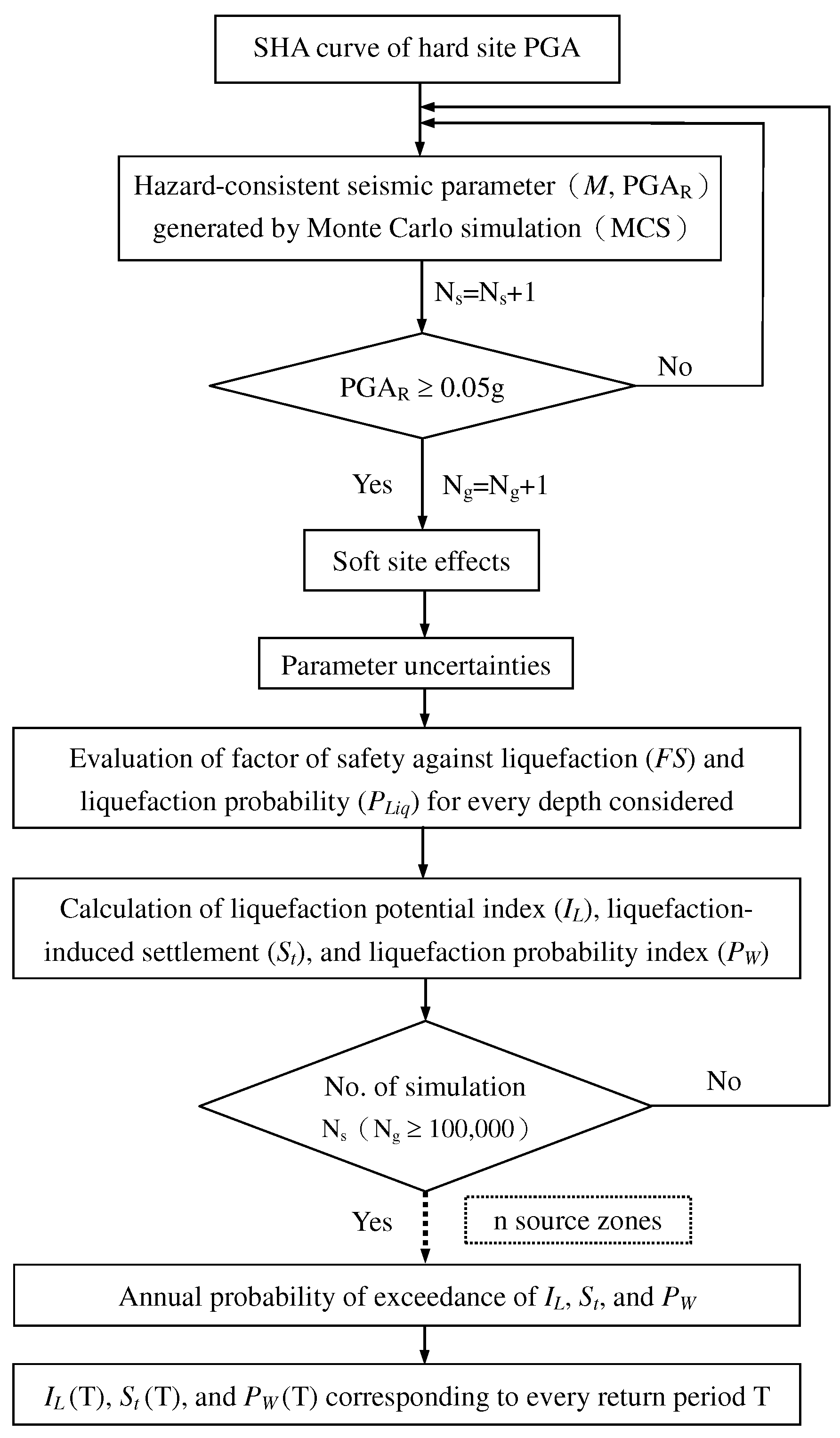
3.2. Simulation of Hazard-Consistent Seismic Parameters

To produce the pair of seismic parameters that match the hazard level, the earthquake magnitude (M) and the peak ground acceleration (PGA), we first simulate the magnitude, M, of a seismic event and the distance from the site to the source, R. Then, we use Equation (14) to calculate the horizontal peak ground acceleration, PGA_R, at the hard site for the given scenario of M and R. This way, we obtain the pair of (M, PGA_R) as well.

Table 4 lists the random variables that the Monte Carlo simulation uses. The seismic sources can be either line sources or area sources, depending on whether they are in the shallow zone or not. For well-defined faults (Type I sources [14]), the model uses line sources with known parameters such as position, direction and length of the fault line, for example, Type I active fault in Taiwan. The random variables for this type of source are magnitude (M), epicentral distance (R_e), hypocentral depth (h), and the model error term (E). The future seismic events may start a rupture at any location along the fault line. The rupture length of the future events depends on magnitude M.

For area sources, we can use a line source to represent them, but we have to account for the uncertainty of the line source's location and orientation (Type III source [14]). The fault line's length depends on the magnitude M. The random variables in this case are the magnitude (M), the depth of the hypocenter (h), the direction of the fault rupture (θ), and the model error term (E). We can divide the source areas into grid points and assume that each grid point can be the origin of a fault rupture. Therefore, we only use the depth of the hypocenter (h) as a random variable to capture the uncertainty of the seismic event's position.

If the seismic sources are located in a deep zone, they can be approximated as point sources. In this case, the position error may exceed the rupture length, and the hypocentral distance is large enough to make the rupture length negligible. Thus, the only random variables to consider are the magnitude (M), the hypocentral depth (h), and the model error term (E).

The aforementioned random variables follow different distributions. The probability density function of earthquake magnitude, M, is [14]

f_{M} (m) = {\begin{cases} 0 & f o r m \leq M_{0} \\ \frac{2.3 b \exp [- 2.3 b (m - M_{0})]}{1 - \exp [- 2.3 b (M_{u} - M_{0})]} & f o r M_{0} < m \leq M_{u} \\ 0 & f o r m > M_{u} \end{cases}

(17)

where b is the seismic region coefficient;

M_{0}

and

M_{u}

are the smallest magnitude of concern to engineering (5.0 is used in this study) and the upper bound magnitude, which depends on the region, respectively.

We assume that the model error term, E, follows a log-normal distribution. The fault rupture azimuth, θ, has a uniform distribution over 2π. For the epicentral distance of R_e and hypocentral depth of h, we also assume that they are uniformly distributed over the range given by the seismic source database.

3.3. Liquefaction Hazard and Fragility Curves

A diagram that illustrates the steps for assessing the risk of liquefaction is presented in Figure 2. The process begins by randomly creating a set of seismic parameters that are compatible with the hazard level, namely the earthquake magnitude, M, and the corresponding peak ground acceleration at stiff sites, . These parameters are then used to evaluate the liquefaction potential.

In the following, after considering the soft site effects and the uncertainties of associated parameters of geological data, the factor of safety against liquefaction (FS) and the liquefaction probability (P_Liq) for every depth considered are first computed. Then, the liquefaction potential index (I_L), liquefaction-induced settlement (S_t), and the liquefaction probability index (P_W) are calculated as follows to evaluate the liquefaction damage of the site subject to earthquake.

The system will only process the samples of PGA_R ≥ 0.05g to assess the liquefaction damage level of the site. The soil is considered to be non-liquefiable if it has a factor of safety above 1.0 and a zero liquefaction probability for the sample of PGA_R < 0.05g. The simulation runs until the number of samples of PGA_R ≥ 0.05g, denoted by Ng, exceeds 100,000.

If we denote the damage index of liquefaction as X, and assume that the occurrences of earthquakes follow the Poisson process, the annual probability of the damage index exceeding a specified state x can be expressed as

P {[X > x]}_{1 y e a r} = 1 - \exp {- \sum_{i = 1}^{n} P [X > x | E_{i}] \cdot v_{i}}

(18)

The symbols above are the same as those in Equation (16).

Based on the flowchart of the liquefaction hazard analysis shown in Figure 3 and the Equation (18), the damage state of the liquefaction for any specified return period T can be obtained as a reference for the engineering design. On the other hand, to meet the requirements of seismic scenario simulation and the early warning system for liquefaction damages, the fragility curves of the liquefaction of the site are another important part to be determined. As to how to build the fragility curves, the partial procedures are the same as those in Figure 3. When the pair of seismic parameters (M, PGA_R) is generated, the soft site effects and the uncertainties of the associated parameters of the geological data are considered, and then the damage indices (I_L, S_t, and P_W) are calculated, the following equation is used to estimate the liquefaction fragility corresponding to a specified peak ground acceleration value of a:

\hat{F} (x; a) = \hat{P} [X > x| IM = a] = \frac{No of (X_{i} > x)}{No of (a - \frac{∆ a}{2} < {IM}_{i} < a + \frac{∆ a}{2})}

(19)

In which IM_i and X_i are the i^th Monte Carlo simulation values of PGA_R and the corresponding damage index, respectively. Δa is the interval of PGA_R considered. The value of 0.02 g is adopted in this study.

4. Case Study

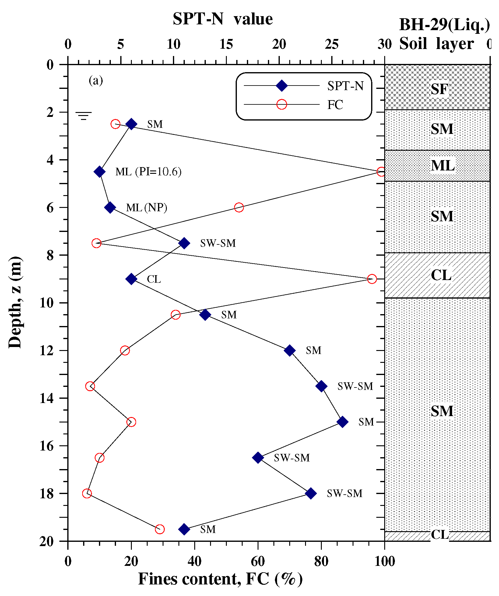
4.1. Site Condition

On 21 September 1999, the largest earthquake of the 20^th century in Taiwan (Mw = 7.6, M_L = 7.3) struck this island. The epicentre was near Chi-Chi, so it has been named the Chi-Chi earthquake. The earthquake killed more than 2400 people and caused serious damage to buildings, bridges, dams, and infrastructures. One of the causes of the severe damage to the structures was soil liquefaction and ground settlement during the earthquake. After the earthquake, Moh and Associates (MAA) [17,18] conducted a detailed site investigation at liquefaction sites and neighbouring zones, including Yuanlin city of Changhua county. Of these site investigation data, one borehole labelled BH-29 with definite evidence of liquefaction is taken as an example in this study to demonstrate the build-up of fragility curves for soil liquefaction and its application. The borehole site of BH-29 is located in an old well filled with boiling sand during the Chi-Chi earthquake.

The soil profile of the BH-29 site is shown in Figure 4. According to the condition of the site under investigation, to a depth of 20 m below the ground surface, the majority consisted of alluvium silty sands and silts, except for the depths of 7.9~9.8m and 19.6~20.0m with clay. The SPT-N values are below 10 within shallow depths. The groundwater table is located at a depth of 2.0 m.

For the Chinan Plain in Taiwan, the relationship of PGA between the soft site and the hard site conditions is shown in Figure 5 [3]. Because the BH-29 site is near the Chinan Plain, the median relationship curve in Figure 5 is adopted to consider the soft site effects when evaluating the seismic fragility of soil liquefaction. On the other hand, uncertainties about the SPT-N value and groundwater table will be included in the analyses.

4.2. Liquefaction Fragility

According to the flowchart of liquefaction hazard analysis shown in Figure 3, Equation (19), and the site condition of the BH-29 site, the fragility curves and the corresponding probability density of the liquefaction potential index (I_L), the liquefaction-induced settlement (S_t), and the liquefaction probability index (P_W) are shown in Figure 6, Figure 7 and Figure 8, respectively. If the PGA of the design earthquake is 0.3g and “Medium damage” or “Moderate liquefaction” is selected for reference, i.e., I_L≥10, S_t ≥20cm, and P_W≥0.5. The corresponding probabilities are 0.98, 0.97, and 0.89 from the fragility curves, respectively. Although these probabilities are different, they are all close to 1.0. The results fully respond to the soil characteristics of the liquefaction site and demonstrate the use of the developed fragility curves. Furthermore, it can be found that the damage state will get higher as the PGA becomes larger from the trend of the histogram of probability density for each damage index. That is, the larger the PGA, the higher the probability of heavy liquefaction damage.

Here, a lognormal cumulative distribution function is assumed to model the fragility curve, F(x;a) in Equation (3), as:

F (x; a) = Φ {[\frac{\ln (a / m)}{ζ}]}_{x}

(20)

in which a represents PGA; m and

ζ

are median and log-standard deviation, respectively; and Φ[⋅]= standardized normal distribution function.

Table 5 shows the two parameters m and

ζ

for the damage indices I_L, S_t, and P_W for several damage levels. It fits very well when comparing regression curves and data points, obtained from Equation (19), as shown in Figure 6, Figure 7 and Figure 8.

From Table 5, we can find that the median m is large when the damage level becomes high, whereas the log-standard deviation does not have this common trend.

5. Conclusions

This research proposed a method to construct hazard-consistent fragility curves for soil liquefaction using Monte Carlo simulation. The seismic parameters for evaluating liquefaction damage are the pair of earthquake magnitude and associated peak ground acceleration (M, PGA). The results of the liquefaction potential and damages thus obtained are more reasonable.
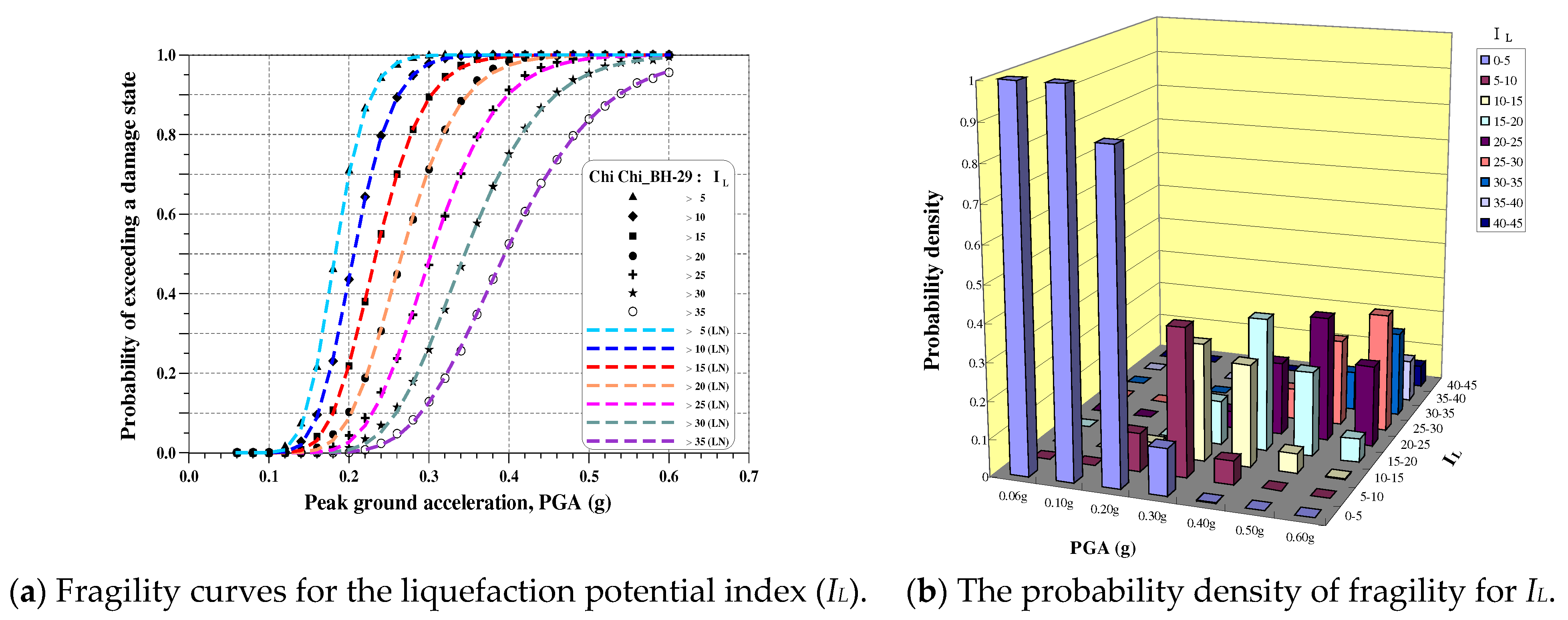
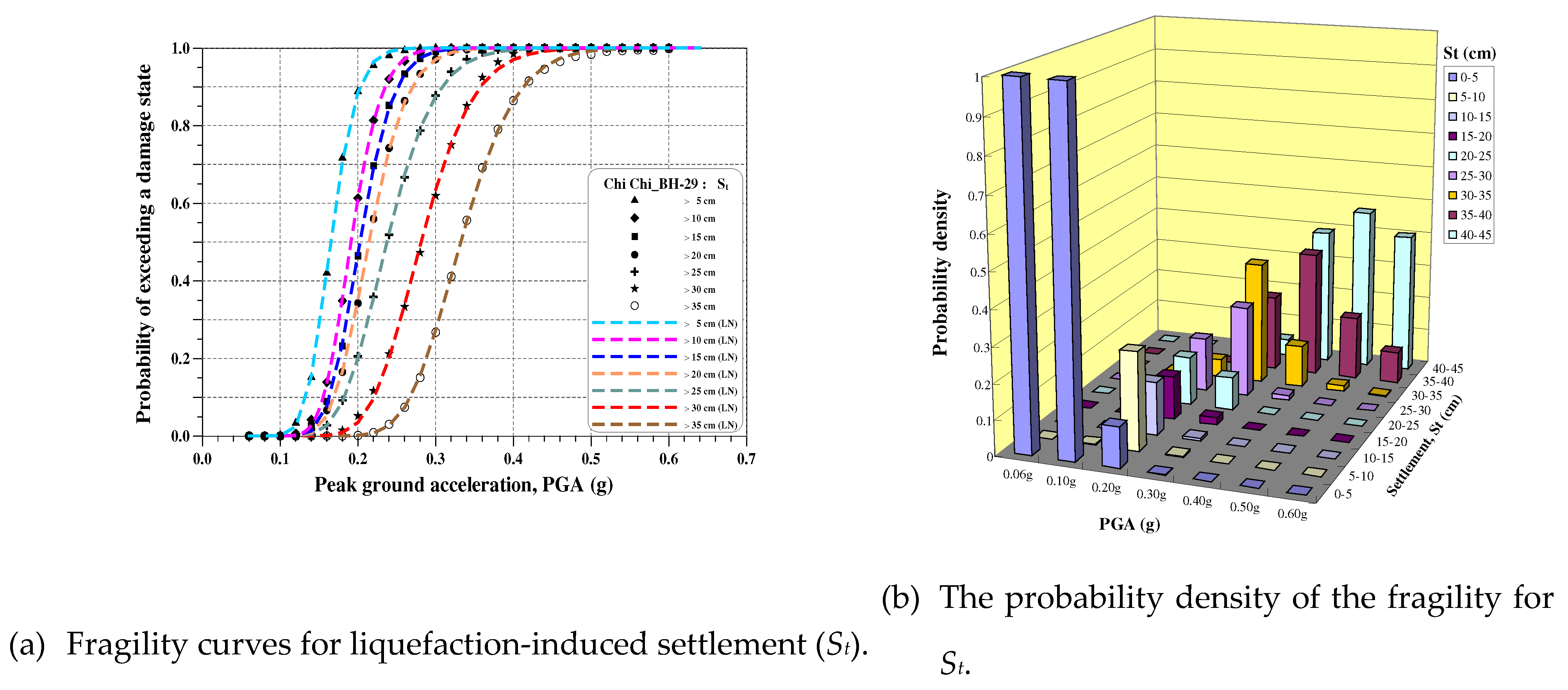
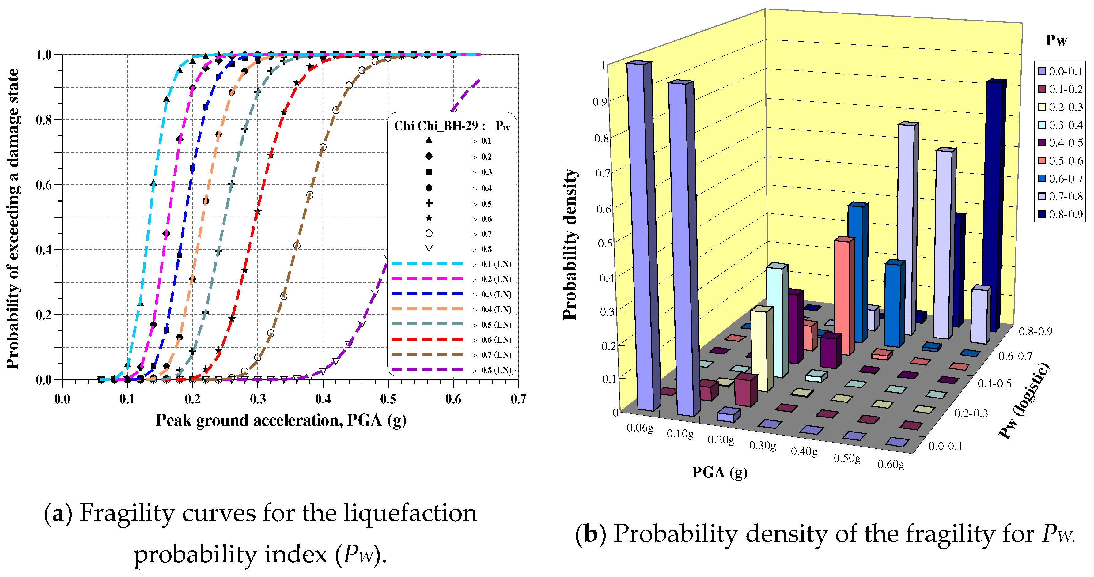
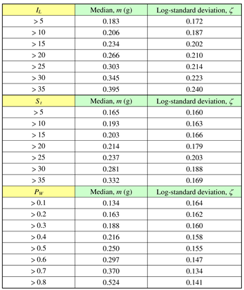
According to the results of the analysis of the case study for the sand-boil site located in Yuanlin city in Changhua county, the liquefaction potential index, I_L, the settlement after liquefaction, S_t, and the liquefaction probability index, P_W, have been shown to be appropriate parameters to assess the damage of liquefaction and to build fragility curves.
By the hazard-consistent fragility curves of soil liquefaction developed here, a tool of scenario simulation for liquefaction damage is provided. It will be beneficial to the “Taiwan Earthquake Loss Estimation System”－TELES. Furthermore, it can serve as a guide for the decision-making of countermeasure design against liquefaction.

References

Cubrinovski, M.; Ntritsos, N. 8th Ishihara lecture: holistic evaluation of liquefaction response. Soil Dyn. Earthq. Eng. 2023, 168, 107777. [Google Scholar] [CrossRef]
Ko, Y.Y.; Tsai, C.C.; Hwang, J.H.; Hwang, Y.W.; Ge, L.; Chu, M.C. Failure of engineering structures and associated geotechnical problems during the 2022 M_L 6.8 Chihshang earthquake, Taiwan. Nat. Hazards 2023, 118, 55–94. [Google Scholar] [CrossRef]
Huang, F.K. Analysis for Seismic Risk of Soil Liquefaction, Ph.D. Dissertation, National Taiwan University, Taipei, Taiwan, 1996. [Google Scholar]
Yeh, C.H. Taiwan Earthquake Loss Estimation System–TELES, Report No. NCREE-03-002, National Center for Research on Earthquake Engineering, Taipei, Taiwan, 2003.
Risk Management Solutions, Inc., Earthquake Loss Estimation Method－HAZUS97 Technical Manual, National Institute of Building Sciences, Washington, DC, 1997.
Iwasaki, T.; Arakawa, T.; Tokida, K. Simplified procedures for assessing soil liquefaction during earthquake. In Proceedings of the Conference on Soil Dynamics and Earthquake Engineering, Southampton, 13–15 July 1982; pp. 925–939. [Google Scholar]
Ishihara, K.; Yoshimine, M. Evaluation of settlements in sand deposits following liquefaction during earthquakes. Soils Found. 1992, 32, 173–188. [Google Scholar] [CrossRef]
Seed, H.B.; Idriss, I.M. Simplified procedure for evaluating soil liquefaction potential. J. Soil Mech. Found. Div. ASCE 1971, 97, 1249–1273. [Google Scholar] [CrossRef]
Youd, T.L.; Idriss, I.M.; Andrus, R.D.; Arango, I.; Castro, G.; Christian, J.T.; Dobry, R.; Finn, W.D.L; Harder, L. F., Jr.; Hynes, M.E.; Ishihara, K.; Koester, J.P.; Laio, S.S.C.; Marcuson, W.F., III; Martin, G.R.; Mitchell, J.K.; Moriwaki, Y.; Power, M.S.; Robertson, P.K.; Seed, R.B.; Stokoe, II, K.H. Liquefaction resistance of soils: summary report from the 1996 NCEER and 1998 NCEER/NSF workshops on evaluation of liquefaction resistance of soils. J. Geotech. Geoenviron. Eng. ASCE 2001, 127, 817–833. [Google Scholar] [CrossRef]
Huang, F.K. Establishment and application of the evaluation model for the liquefaction probability and associated damages based on the information theory. J. Chin. Inst. Civ. Hydraul. Eng. 2008, 20, 301–314. [Google Scholar]
Huang, F.K. Establishment and application of the SPT evaluation model for the liquefaction probability and associated damages. J. Chin. Inst. Civ. Hydraul. Eng. 2008, 20, 155–174. [Google Scholar]
Reiter, L. Earthquake Hazard Analysis: Issues and Insights, Columbia University Press, New York, 1990.
Cornell, C.A. Engineering seismic risk analysis. Bull. Seismol. Soc. Am. 1968, 58, 1583–1606. [Google Scholar] [CrossRef]
Der Kiureghian, A.; Ang, A.H.-S. Fault rupture model for seismic risk analysis. Bull. Seismol. Soc. Am. 1997, 67, 1173–1194. [Google Scholar]
Campbell, K.W. Near-source attenuation of peak horizontal acceleration. Bull. Seismol. Soc. Am. 1981, 71, 2039–2070. [Google Scholar]
Jean, W.Y.; Chang, Y. W.; Loh, C. H. Early Estimation Procedure for the Potential of Seismic Disaster, Report No. NCREE-04-001, pp.67-72, National Center for Research on Earthquake Engineering, Taipei, Taiwan, 2004.
Moh and Associates (MAA), Soil Liquefaction Assessment and Remediation Study, Phase I (Yuanlin, Dachun, and Shetou), Summary Report and Appendices, Moh and Associates (MAA), Inc., Taipei, Taiwan (in Chinese), 2000.
Moh and Associates (MAA), Soil Liquefaction Investigation in Nantou and Wufeng Areas, Moh and Associates (MAA), Inc., Taipei, Taiwan (in Chinese), 2000.

Figure 1. Procedures for seismic hazard analysis.

Figure 2. Seismic zone and epicentral distribution for M>5.0.

Figure 3. Flowchart of liquefaction hazard analysis.

Figure 4. Soil profile of the BH-29 site.

Figure 5. PGA relationship between the soft site and the hard site condition. [3].

Figure 6. Fragility for I_L of the BH-29 site.

Figure 7. Fragility for S_t of the BH-29 site.

Figure 8. Fragility for P_W of the BH-29 site.

Table 1. Liquefaction potential classes based on I_L (Iwasaki et al., 1982) [6].

I_L	Liquefaction potential class
0	Very low
0 < I_L ≤ 5	Low
5 < I_L ≤ 15	High
I_L >15	Very high

Table 2. Relation between the extent of the damage and approximate settlements [7].

Extent of damage	Settlements S_t (cm)	Phenomena on the ground surface
Light to no damage	0 ~ 10	Minor cracks
Medium damage	10 ~ 30	Small cracks, oozing of sand
Extensive damage	30 ~70	Large cracks, spouting of sands, large offsets, lateral movement

Table 3. Classification of the damage states of liquefaction according to P_W.

Class	P_W	Description of damage state
I	< 0.30	Minor liquefaction
II	0.30 ~ 0.85	Moderate liquefaction
III	> 0.85	Heavy liquefaction

Table 4. Types of seismic sources and random variables.

Table 5. Parameters of the fragility curves of the BH-29 site.

Disclaimer/Publisher’s Note: The statements, opinions and data contained in all publications are solely those of the individual author(s) and contributor(s) and not of MDPI and/or the editor(s). MDPI and/or the editor(s) disclaim responsibility for any injury to people or property resulting from any ideas, methods, instructions or products referred to in the content.

© 2023 by the authors. Licensee MDPI, Basel, Switzerland. This article is an open access article distributed under the terms and conditions of the Creative Commons Attribution (CC BY) license (http://creativecommons.org/licenses/by/4.0/).

Copyright: This open access article is published under a Creative Commons CC BY 4.0 license, which permit the free download, distribution, and reuse, provided that the author and preprint are cited in any reuse.

Alerts

MDPI Initiatives

Important Links

Choose an area of interest and we will send you notifications of new preprints at your preferred frequency.

Disclaimer

A Method for Developing Fragility Curves for Soil Liquefaction Consistent with the Seismic Hazard Using Monte Carlo Simulation

Abstract

Keywords:

Subject:

1. Introduction

2. Liquefaction Fragility

2.1. Fragility Assessment Method

2.2. Damage Evaluation of Soil Liquefaction

3. Hazard-Consistent Fragility Curves of Soil Liquefaction

3.1. Procedures for Seismic Hazard Analysis

3.2. Simulation of Hazard-Consistent Seismic Parameters

3.3. Liquefaction Hazard and Fragility Curves

4. Case Study

4.1. Site Condition

4.2. Liquefaction Fragility

5. Conclusions

References

MDPI Initiatives

Important Links

Subscribe