1. Introduction and motivation
The air pollution represents a common concern worldwide, and the air quality might change from place to another based on the intensification of its sources that may be natural or anthropogenic. The intensification of anthropogenic sources of air pollution and other natural sources have a great concern on the air quality. Air pollution has negative effects not only on human health but also on animals, plants, ecosystems, and global warming. The annual premature deaths due to outdoor and indoor air pollution were found to be 3.7 and 4.3 million, respectively ([
49]).
In the literature, the particulate matter (PM) was considered as the most important air pollutant, especially the fine and ultrafine air particulates which are associated with respiratory diseases and cardiovascular mortality ([
13,
16,
17]). The size of particulate matter has attracted a remarkable attention in bibliography since the fine particulates have an important impact on global climate due to their long life in the atmosphere and transport efficiencies ([
28,
35,
36]). Moreover, recent large scale epidemiological studies ([
16,
45]) have clearly demonstrated a correlation of the increased concentration of fine particulates in the atmosphere with the appearance of harmful and adverse effects on human population. Indeed, based on many epidemiological studies, the mass concentration of the fine particulate matter in the atmosphere is proportional to the appearance of harmful and adverse diseases. The fine particulate matter with an aerodynamic diameter equal or less than 2.5
(PM2.5) has gained a lot of attention in the literature because it can stay in the atmosphere a long time and travel thousands of kilometers. The long-term exposure to the PM2.5 aerosols may drastically influence lung function and cause chronic bronchitis, heart disease, and lung cancer especially for children and elderly. Furthermore, the characterization of fractionated atmospheric aerosols is important because the chemical composition and the quantities of trace elements may vary with the sources of particles as well as with the size of atmospheric aerosols collected. The study of PM2.5 and PM10 fraction in particular has taken a lot of attention in the literature ([
25,
37,
38,
46]).
In the Middle East, especially, (e.g. Greater Cairo - Egypt, Taif and Makkah - Saudi Arabia), atmospheric aerosol samples have been studied extensively ([
27,
40,
41,
42,
43,
44]). Recall that, indeed, the Middle East region is facing important changes in climate, and the need to desalinated water and cooling are major interests nowadays due to their great impact on many activities such as the change to green lands, agriculture, tourism, and so on. For example, greenhouse gas emission is known to be very high in the Middle East region due to the region’s economic reliance on carbon-intensive industries. United Arab Emirates and Saudi Arabia are considered as important contributors to these regional emissions.
The knowledge of the chemical composition of air particulate matter is very important. It gives important information on their origin and also reveals whether they were emitted as primary or secondary particles. The smaller the particle, the more harm it may cause, as it penetrates deep into the lungs. The bulk of these particles originates from anthropogenic emissions, both directly and as secondary formation in the atmosphere from gases like SO2, NOx and volatile organic compounds. The local emission of fine particles can become an issue of regional and even global concern, since these particles are able to affect air quality in other countries through transnational and even transcontinental transport. Black carbon represents also one of the main air pollution whereas it is produced by incomplete combustion and always mixed with other atmospheric constituents. Generally, there are two important aspects for knowing the elemental content in air particulate matters. First there are heavy elements that are in themselves toxic to human health. It is of interest to follow the ecocycles of these metals as environmental hazards, once they are released into the atmosphere, biosphere and technosphere. The second aspect is that single elements or ratios between elements can be used as a fingerprint of a special source emitting other hazardous species that are less stable and more difficult to measure.
The present work aims to develop a quantitative/mathematical model to air quality index measuring based on time series analysis. A regression model will be tested for the impact of the time scale behavior and the multifractality of both the AQI and its components. The main mathematical tool to be applied is wavelet multiresolution analysis. Recall that wavelets are mathematical toolkits that have shown since their appearance an efficiency and success in the time series analysis and the exploration of their properties such as nonstationarity, fluctuations, dynamics, multifractality, and so on.
The data to be applied will be based on samples collected from the cities of Tabuk region, Saudi Arabia in order to evaluate the air quality in this region.
2. Wavelets for time series processing
Wavelet analysis is a refinement of Fourier analysis developed in the last decades and applied in many scientific fields. It therefore proved its efficiency and performance as a mathematical quantitative tool.
The main principle in wavelet theory of time series is the breaking down or the decomposition of time series into subseries
where
is known as the breaking level, and the components
and
,
are projections of the original series
S on some special subspaces of the whole space
composed of all time series with finite variance. More precisely,
is expressed by means of an orthogonal basis
of a special space
known as the approximation space at the level
j as
where the coefficients
are the so-called approximation or scaling coefficients of
S at the level
j and the position
k, evaluated by means of the discrete convolution
Similarly,
is expressed by means of an orthogonal basis
of a special space
known as the detail space at the level
j as
where the coefficients
are the so-called wavelet or detail coefficients (or also the discrete wavelet transform) of
S at the level
j and the position
k, evaluated by means of the discrete convolution
In general, the orthogonal bases above are issued from one source couple of functions
known as the (father or scaling,mother) wavelet by setting
By noticing that
and
, we get an orthogonal decomposition
. The series
S will be decomposed in a whole wavelet series decomposition
relative to a fixed integer
.
In practice, obviously, a restriction a maximal level is needed. For this we fix
and consider the approximation
The lower index is in fact more flexible, does not have an important effect on the total decomposition and usually chosen to be 0. The choice of J is always critical, and is related to the eventual error estimates relative to the error applied to get the closeness of to the origin S.
To be familiar with wavelets, their properties, and the necessary assumptions for a function to be a (father,mother) wavelet, the readers may refer to [
7,
8]).
2.1. Backward-forward wavelet time series completion
One of the major problems in data analysis is the missing data drawback. This is widely confronted in many fields such as financial time series, climate time series, and so on. It may be also due to the uncertainty of some parts of the data samples to be applied. Uncertain values are generally omitted and thus lead to missing data in the sample. To overcome this problem, many mathematical tools have been applied to complete the gaps in data samples such as neural networks, kernels, probabilistic methods, and so on. Moreover, it is noticed that the construction of missing data in quasi all existing studies is based on the usual method starting from a training sample, constructing an approximative model, and then complete the future values of the sample with this model. However, in many cases, the lack or the absence of data may be itself at the beginning of the target period of time to be investigated. This needs therefore to adopt suitable ways to overcome this problem, and gives rise to what we called here a backward-forward method, a black-box that may read the existing values and reconstruct the missing parts in both the past and future of the training segments.
In the present work, we are consequently concerned in a backward-forward wavelet approach to fill the missing data segments, and thus get a complete eventual sample to be applied by the next in the analysis.
Let
,
, be a time series (due to some AQI factors) decomposed in a wavelet series decomposition at a level
J, relative to a wavelet system
, (as in
8, with
chosen for the sake of simplicity),
The missing values are classified into two classes. We call a backward missing value any value , for which there is a known segment after it, but an unknown one before it. Similarly, a foreword missing value will be preceded by a segment of known values, and proceeded by a segment of unknown values. A missing value that is isolated will be called just a middle missing value.
To reconstruct a backward missing value
, denote
the length of the segment
of known values that follow it. We construct the so-called backward approximation and detail coefficients as
Similarly, for a forward missing value
, the forward approximation and detail coefficients are built as
Whenever is a middle missing value, the higher length backward/forward interval is chosen, and the previous steps are applied. In the case of the equality of lengths, a mean value is computed.
Each predicted value is added to the series, and the new series is re-considered for the next steps.
Here,
is the wavelet kernel associated to the couple
. We thus, contrarily to the majority of existing works, we act a forecasting process on the wavelet/scaling coefficients of the series instead to the series itself. The forecasted value of the series
X will be obtained by adding the components relative to the forecasted coefficients above. A similar idea is already developed in [
6,
9,
10].
3. Exploring the multifractality in time series
Time series hide many characters such as tails or stylized facts due to hidden characters of the data itself, such as the uncertainty, the randomness, the stochasticity, scaling laws, leptokurticity, and so on. These characteristics may be described via the series itself or its variance by means of the so-called volatility.
To understand the behavior of time series and thus the data behind them, suitable tools have to be acted. The ’last’ tool applied in this context is the fractal analysis and its last version known as the wavelet multifractal analysis. Such an analysis aims to describe or to confirm the fractal/multifractal structure of the data by evaluating the so-called multifractal spectrum of the time series associated starting with the evaluation of the time series means of the
q-increments as
This gives the she scaling law function
obtained by regressing
against the log time step
to obtain
The multifractal spectrum is evaluated as the Legendre transform of the function
as
Whenever is linear, we say that the time series is fractal (or mono-fractal), while for a nonlinear scaling law function , we get a multifractal time series, with a multifractal spectrum being concave or equivalently with a concave scaling law function .
Recently, wavelets have been involved in the evaluation of the multifractal structures of time series benefiting from the functional framework by replacing the partition function above with a wavelet-based variant (depending on the level of decomposition
j) as
where the
are the wavelet coefficients (detail) or sometimes the wavelet leaders of the time series
. This leads to the analogue scaling law function
as
Backgrounds and details on multifractal analysis of time series, and extensions may be found in [
7,
11,
12].
4. The air quality index modeling
In this part, we will examine the AQI index as a time series to emphasize the dependence on the time scale in such an index. In the literature, the AQI depends essentially on the following factors,
PM2.5 designating particulate matter with 2.5 microns or less in diameter.
PM10 representing particulate matter with 10 microns or less in diameter.
SO2, the sulfur dioxide,
NO2, the nitrogen dioxide,
CO, the carbon monoxide,
O3, the ground level ozone.
Besides, in the literature, all existing works considered the mathematical model
to compute the overall AQI. This model, even-though it is widely applied, it presents many drawbacks. Indeed, it means (at least locally) that one factor is involved for the computation of the air quality, the one having the larger value. However, this fact does not describe the real climate phenomenon. In the nature, there are many factors hidden which are not clearly involved in the quantitative models, and which moreover may be stochastic or even chaotic. These behaviors impact severely the maximum value which may be itself chaotic or presents extreme values. In addition, the max model has a drawback related to the time-scale behavior (fractal, multifractal structure) of its associated time series. Indeed, we know that for a set of many time series, the Hurst-Hölder exponent of the pointwise maximum series is evaluated as the lower bound of the exponents of the different series in the set. This fact may not allow to discover the pointwise behaviour of each component. Moreover, in many cases, it may hide the real structure hidden in the data when resulting in a regular min/max regardless of the multifractality of the components.
To overcome these limitations or disadvantages, we proposed instead of the max model (
13) a modified version of the AQI index already explained by means of the same exogenous factors above, in the form of a weighted combination (superposition) as
where
,
are for the moment constant weights, and
is an error term.
The idea consists in projecting equation (
14) on the detail and approximation spaces according to the level
j to get a
j-level time scale model as
The evaluation of such a model will inform us about the hidden dependence of the AQI and components on the time scale, by evaluating for each level the coefficients , . We expect that the findings will result in a non uniform dependence on the time scale, and thus the dynamics of the factors behind the AQI level are strongly related to the time scale.
5. Empirical results and discussions
In this part, we will examine the AQI index relative to the Saudi Arabia case in the special north west region of Tabuk. The dependence on the time scale always hidden, and not explained explicitly in the mathematical model will be investigated. Therefore, empirical investigations remain necessary to check such a dependence and influence. We aim to test the presence or not of a multifractal structure of such index and/or its components.
5.1. The data sample
The data to be applied will be composed of the principal components of the AQI as recalled previously in (
13) and (
14). Tabuk region contains in fact many stations designated to measure the AQI, such as the stations in Tabuk city itself, Haql city, Umluj city, Alwajh city, and Tayma city. In front of a nonavailability of a main authority providing the needed data, the data is gathered manually from many websites such as [
50,
51,
52]. Our collection of data resulted in samples traded on the period from July 2019 to December 2021, based on the two stations of Tabuk/Alwajh and Tabuk/Tayma according to the availability of data. However, the samples lacks for many missing values, which lead us to apply the wavelet reconstruction of missing data introduced in
Section 2.1 via the forecasting model (
10)-(
11) in order to get reasonable time series able for a reasonable analysis.
Table 1 below presents some AQI values and their interpretation for an AQ degree or description. These values are just examples which are not necessarily included in the samples applied, but provided for an overview to the reader for the way of interpreting numerical values of AQI factors in terms of the real state of the climate phenomenon.
The choice of Tabuk region as case of study is motivated by the fact that Tabuk region has great importance in the Kingdom, as geographically it occupies a location overlooking the Red Sea and close to the Egyptian Suez Canal, the main corridor for navigation and maritime trade between East and West continents. Tabuk region also represents the cornerstone of the global NEOM project, which combines trade, tourism and climate studies, and aims to make the Saudia Arabai Kingdom a global destination for investment, tourism and residence, achieving thus some major goals of the Kingdom’s 2030-Vision.
Now, the starting step consists in acting wavelets to reconstruct the missing data. On the total basis, we recorded a number of missing values, some of them are illustrated in
Table 2. A complete and adjusted basis on the period of study is thus obtained and applied by the next.
A second step concerns now the statistical investigation of the data. Therefore,
Table 3 below shows the descriptive statistics of the whole data.
Notice easily from
Table 3 that the skewness is non-vanishing for all the indexes, which rejects the asymmetry hypothesis. More precisely, the AQI and PM10 indicate a longer tail on the right, while O3 indicates a left-side longer tail for Alwajh station in front of right-side longer tail for Tayma station. In addition, Alwajh AQI and O3 are nearly symmetrical. The rest of indexes cases are extremely skewed. For the kurtosis measure, all the indexes intersect a non-normal value and/or behavior (the kurtosis being different from 3). All the indexes indicate heavier tails. We may further notice that the standard deviation measure is high, which reflects the high deviation of the indexes around their mean value, and thus reinforce and motivate the use of wavelet multifractal models. Again, the
test statistics returns a value of
meaning that the data does not fit a normal distribution.
5.2. The wavelet multifractal processing
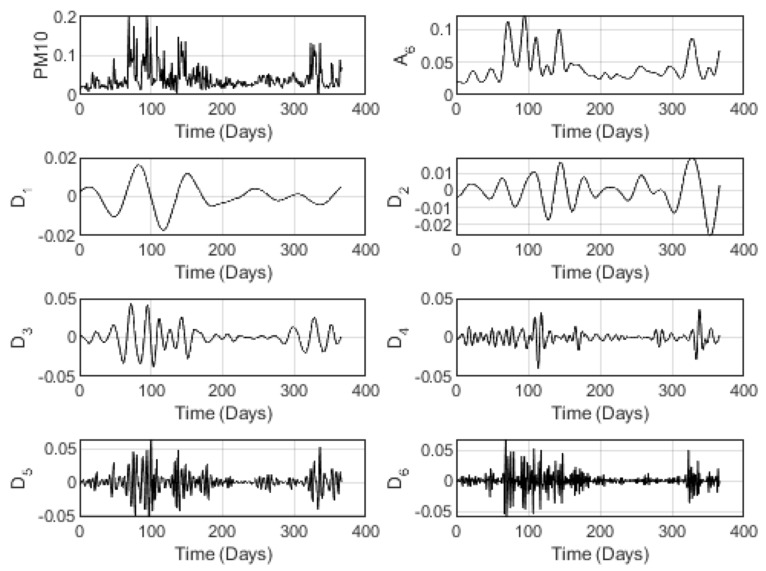
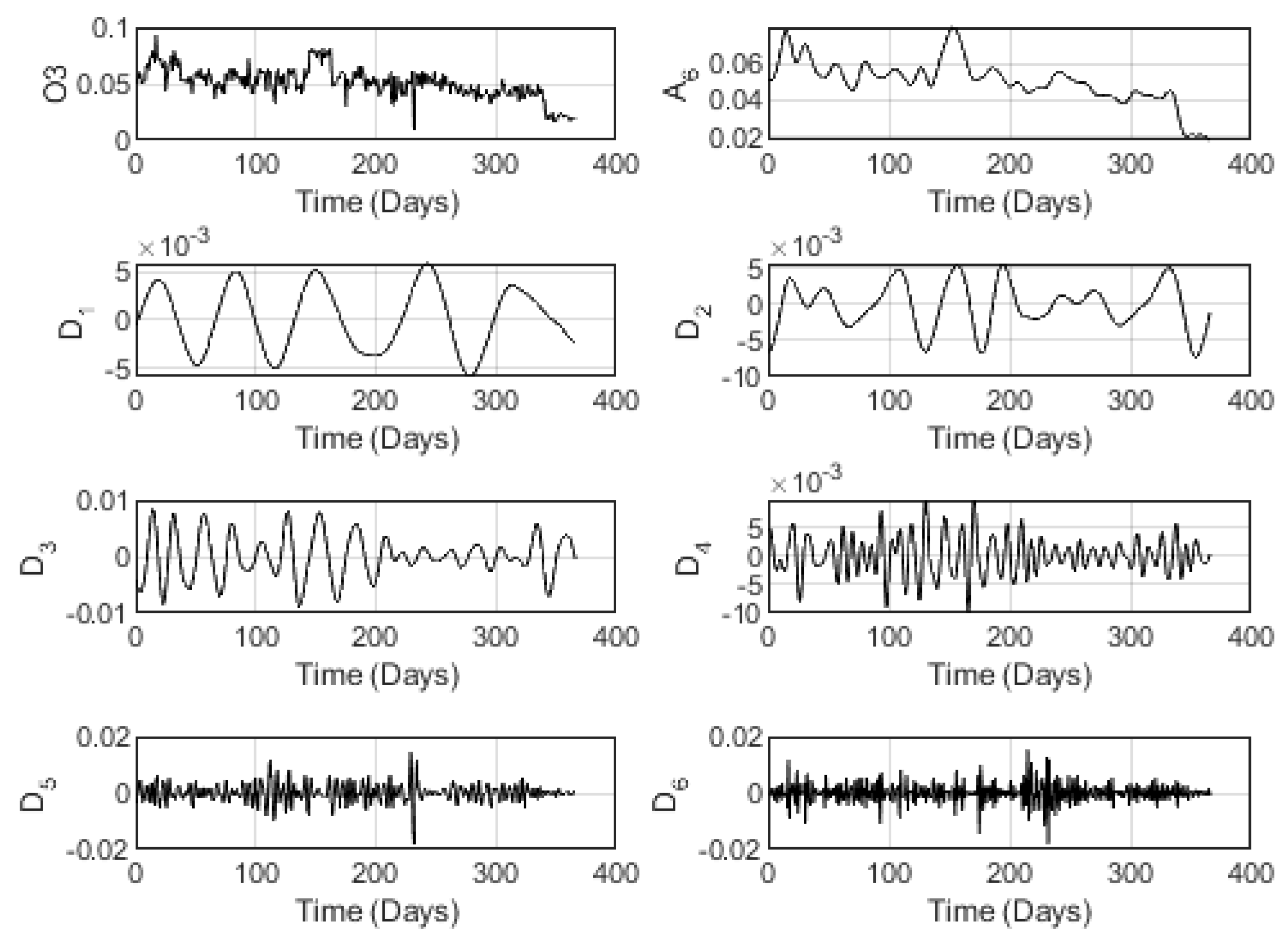
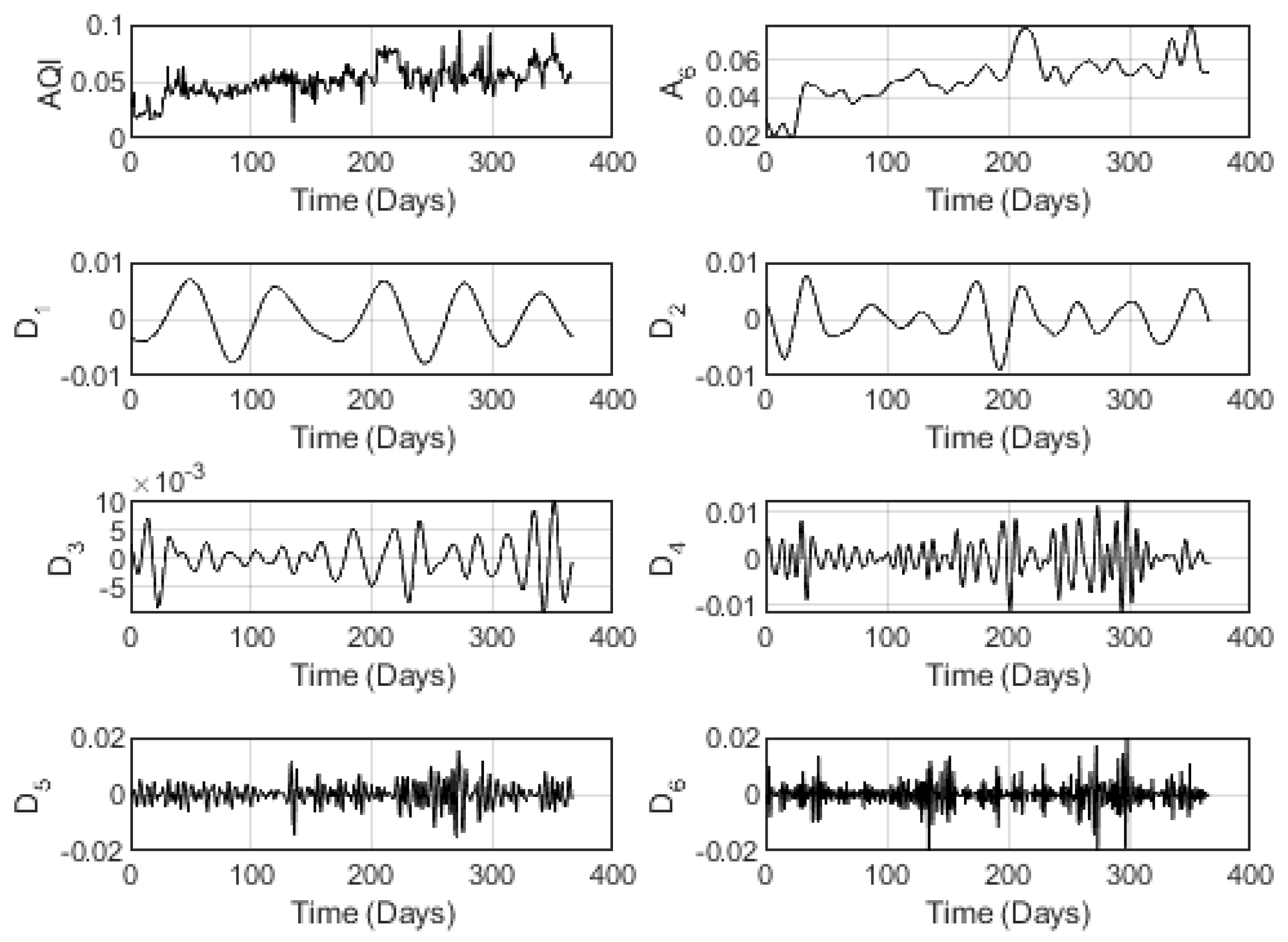
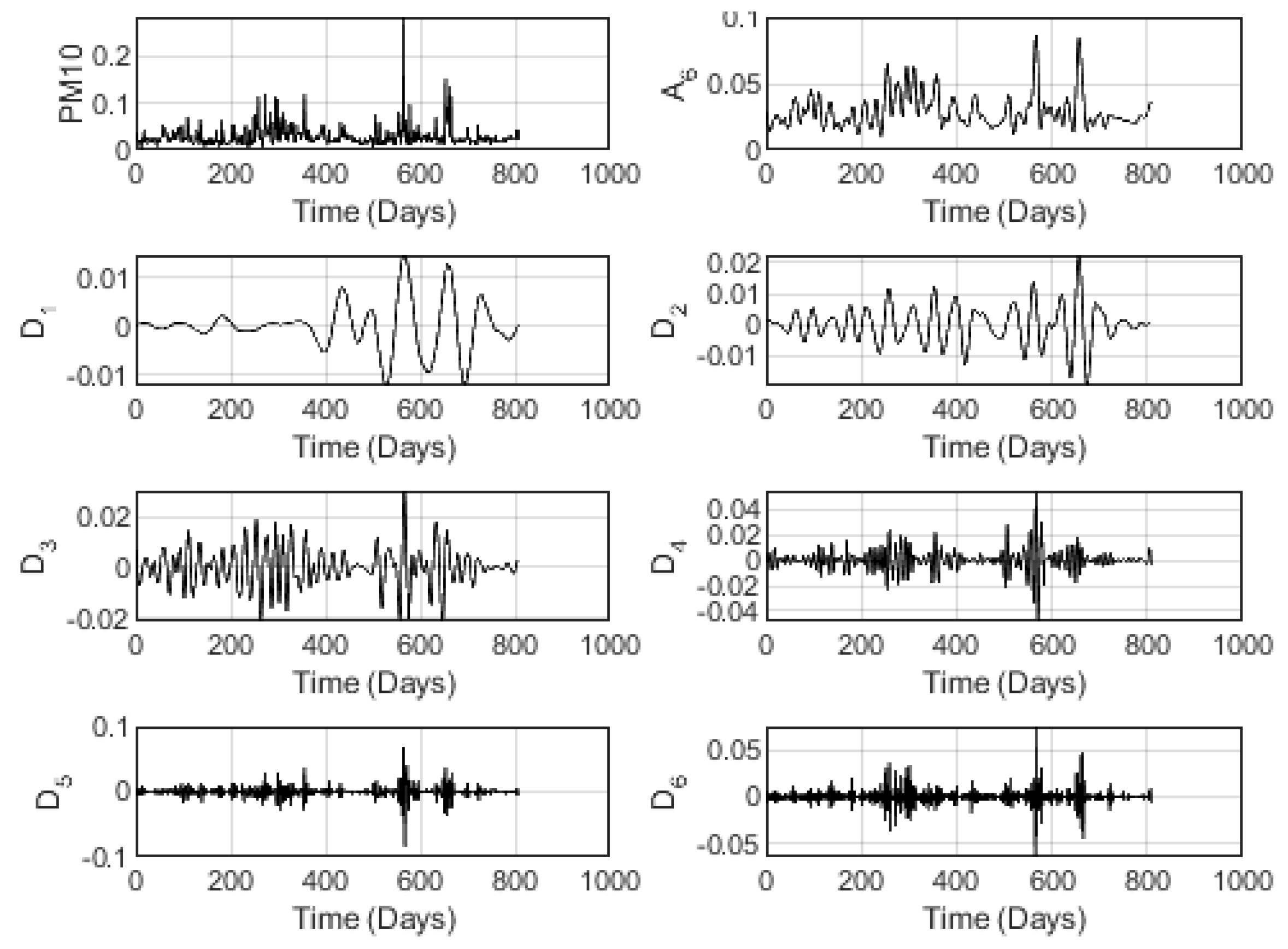
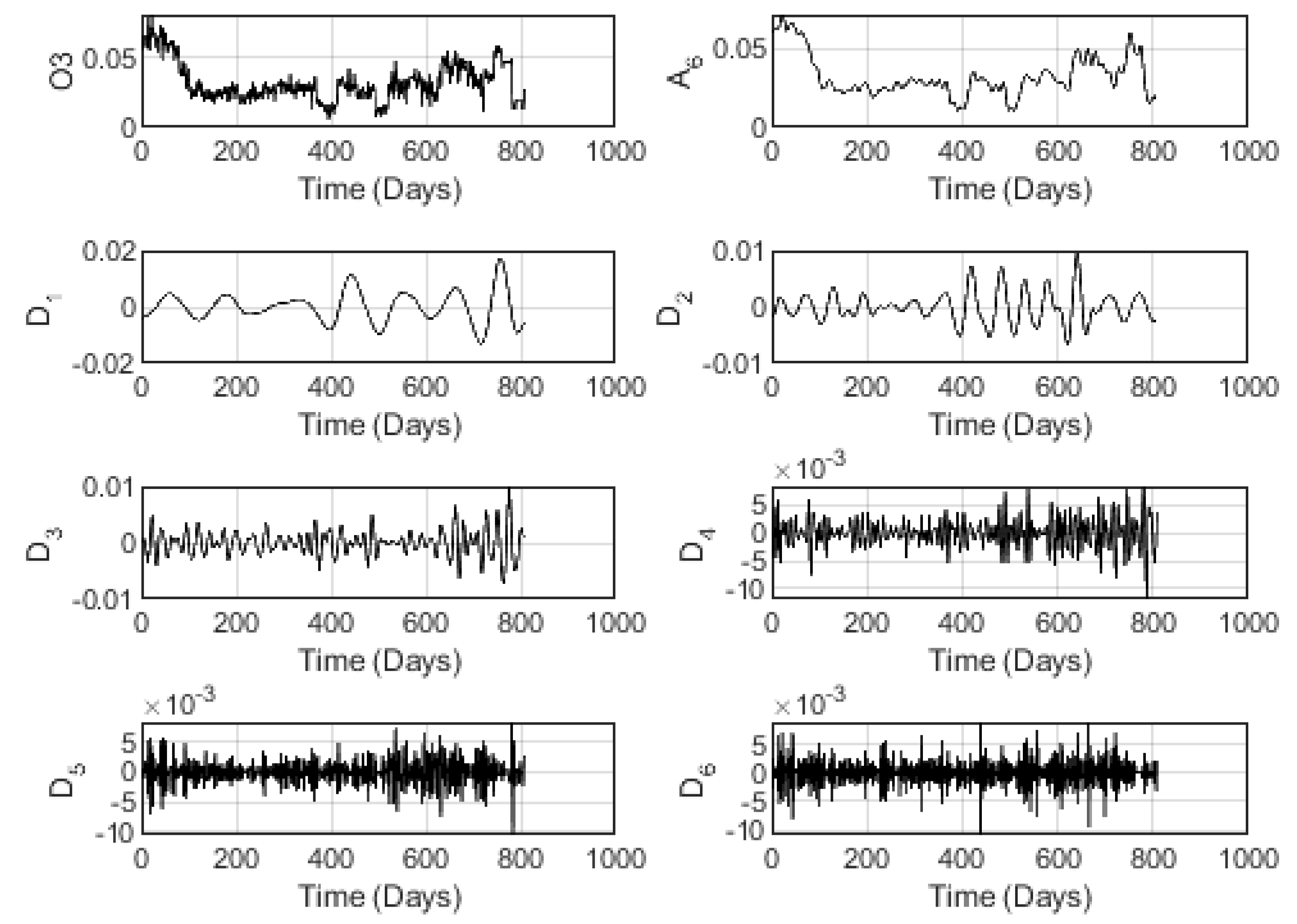
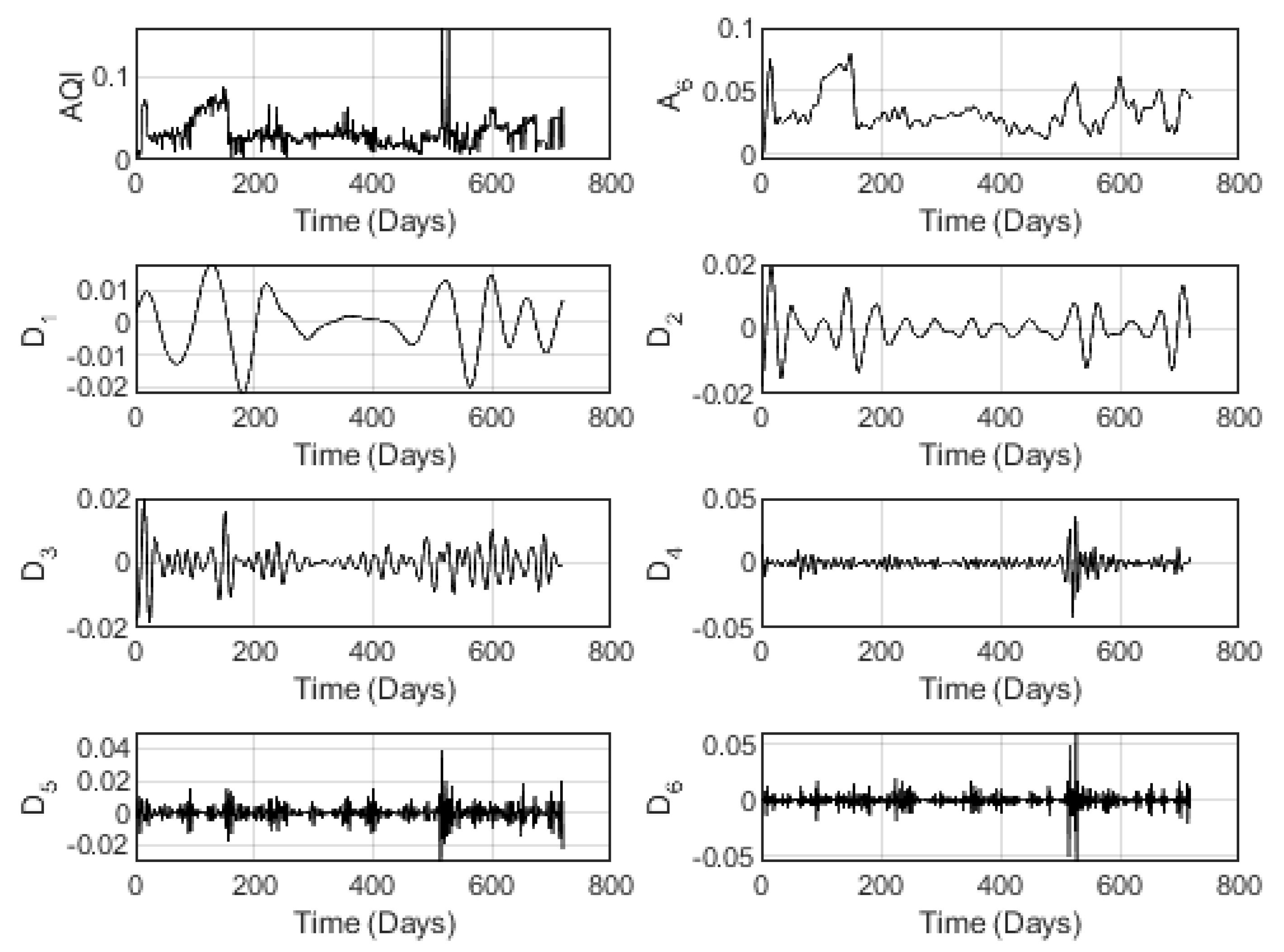
To show how clearly the high volatile aspect of the AQI indexes, a wavelet analysis is conducted in order to appear eventual fluctuations. Such analysis yielded the following Figures relative to the wavelet decomposition at the level 6 by means of a Daubechies DB8 multiresolution analysis.
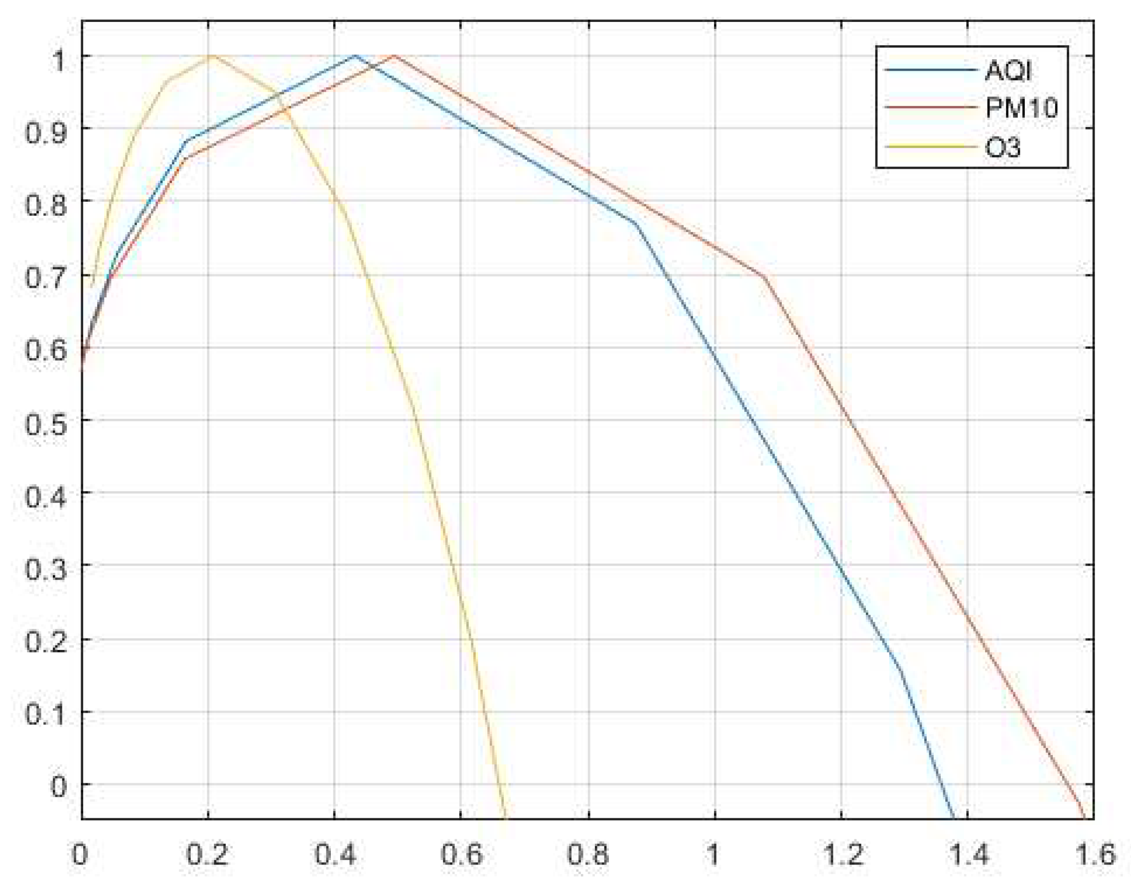
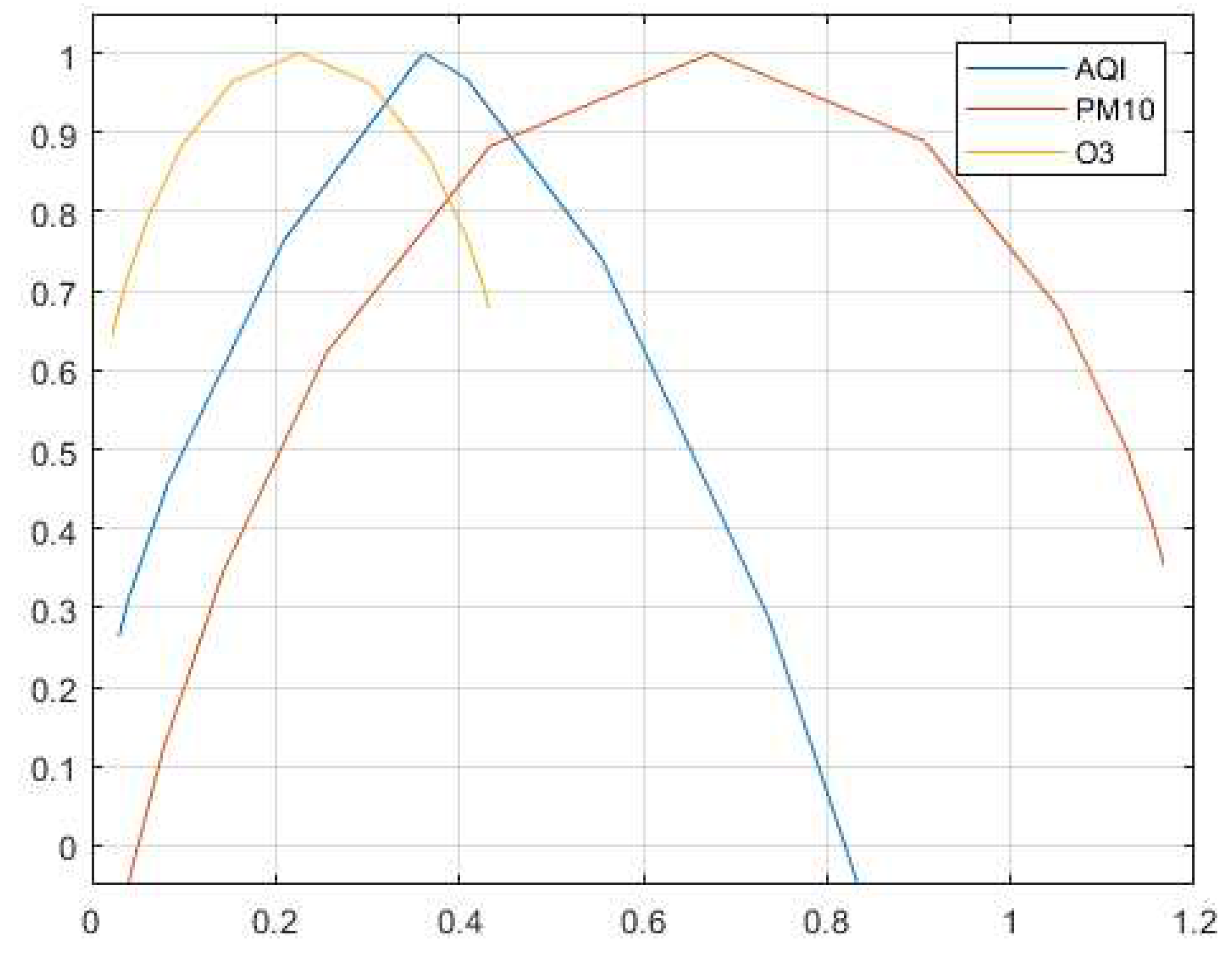
A first test to confirm the multifractal nature of the indexes consists in plotting their wavelet multifractal spectrum introduced in
Section 3.
Figure 1 illustrates the wavelet multifractal spectrum due to the case of Alwajh station, while
Figure 2 illustrates the wavelet multifractal spectrum due to the case of Tayma station.
Notice easily from
Figure 1 and
Figure 2 that concave (nonlinear) spectra are obtained for all the indexes, which confirm effectively the multifractal nature of the data, and motivates the investigation of wavelet analysis to show more precisely the volatile behavior of the indexes.
Figure 3 concerns the multiresolution analysis result due to the PM10 index for Alwajh station conducted at the wavelet decomposition level
.
Figure 4 concerns the wavelet decomposition of the O3 index for Alwajh station conducted also at the wavelet decomposition level
. Besides,
Figure 5 illustrates the wavelet decomposition at the level
for the AQI index estimated by Alwajh station.
It is noticeable from the figures above the effective fitting of the wavelet approximation component of all the indexes, where the general shape is clearly followed by the 6-level tendency. Besides, the wavelet detail components show the fluctuations hidden in the data. Notice that such fluctuations get clearer as the level of decomposition gets larger.
Next, similarly to the previous wavelet multiresolution analysis,
Figure 6 concerns the multiresolution analysis result due to the PM10 index for Tayma station conducted at the wavelet decomposition level
.
Figure 7 concerns the wavelet decomposition of the O3 index for Tayma station conducted also at the wavelet decomposition level
. Besides,
Figure 8 illustrates the wavelet decomposition at the level
for the AQI index estimated by Tayma station.
Here-also, we notice the effective fitting of the wavelet approximation component of all the indexes, where the approximation component shows the general tendency of each associated index. Moreover, the wavelet detail components show the volatile behavior of the data. As previously, the volatile structure gets clearer as the level of decomposition gets larger.
Thew volatile behavior of the index is clearly shown, which confirms and enforces the existence of a fractal/multifractal scaling law in the time series associated, and/or its components. We thus proceed as mentioned previously by plotting its Hurst–Hölder exponent or its spectrum of singularities. This is illustrated by
Figure 2 and
Figure 1 below.
Notice from these illustrations that although the wavelet applied is not necessarily non uniform, the indexes show a concave nonlinear scaling functions, or equivalently a nonlinear concave multifractal spectra. This means that the data is multifractally volatile and it represents a point-wise scaling behavior with a point-wise changing Hurst–Hölder exponent. This motivated the application of wavelet tools to explore its structure as well as its behavior.
In the following step, we estimate the coefficients of the model (
14) as well as its wavelet version (
15) for the approximation levels
. The coefficients are provided with their confidence intervals at the level
.
Notice from the
Table 4 that the model (
14) actually results in positive coefficients, which expresses the significant effect of all variables on the air quality index. This confirms our idea and reveals a first difference with the classic model, which indicates that only the maximum index variable is significant. However, the logic of nature itself (climate) is naturally based on a mixture of phenomena and factors that react together instantly. Let us also always note from
Table 4 that the estimates of the model coefficients ((
14)) present variations (even if slight in some cases), which expresses that indeed the model strongly depends of the scaling factor, and therefore, a hidden multifractal structure takes place in the air quality index as well as its components. This structure appears clearly with the increase in the level of wavelet approximation, where details or hidden fluctuations appear more and more. Some coefficients have become negative, with confidence intervals varying from positive to negative.
From the point of view of the link between the AQI and the factors, we notice that the PM2.5, PM10, and SO2 are the most significant factors compared with others, especially for Alwajh case, where the coefficients are very significant. Next, the O3 factor follows at the fourth order in significance. These effects do not negate the main role of the other indicators, which also have positive coefficients in the majority of levels. Besides, we notice some negative but small coefficients meaning effectively the presence of a nonstationary structure in the data, leading to fluctuations.
6. Conclusion
In this paper, we proposed a wavelet multifractal procedure to estimate the AQI as a time series by introducing a regression model instead of the minmax classical model. The idea is issued from the fact that, instantaneously, there are many factors affecting the quality of air, not only the factor having a maximal index. Indeed, the classical model did not answer the real impact when for example many factors have the same index value. The significance of these factors may not be really differentiated. In the new model, each factor is present instantaneously in the evaluation of the air quality, and the significance is interpreted according to an appropriate coefficient.
The theoretical methodology is applied on the case of the Tabuk city situated in the west north of Saudi Arabia as a representative case of study. The study is conducted during a critical period chosen deliberately to contain sub-periods before, during and after the pandemic COVID19. The study shows that contrarily to the existing studies, the involvement of the time scales in the model and the estimations is adequate to understand the situation of the AQI according to the time scale.
During the investigation, wavelets are applied as a suitable mathematical tool to discover the time scale behavior such as the multifractality of the AQI as well as its components. The wavelet multifractal spectrum estimation confirmed effectively the presence of a multifractal structure in the data. Besides, the coefficients of the model are estimated with corresponding confidence intervals with the original model as well as its wavelet versions. The variation of the wavelet level of approximation confirms effectively the adequacy of the model, and the presence of a fluctuated/multifractal structure in the data.
As future direction, we propose to apply fractal functions to improve or to construct more efficient models to describe the AQI time series, and for the aim of forecasting. Future models may include multifractal detrended fluctuation analysis, self-similar models, and/or their extended versions with wavelets.
Funding:
This research the Deputyship for Research & Innovation, Ministry of Education in Saudi Arabia for funding this research work through the project number 0253-1443-S.
Acknowledgments:
The authors extend their appreciation to the Deputyship for Research & Innovation, Ministry of Education in Saudi Arabia for funding this research work through the project number 0253-1443-S.
Author Contributions:
All authors contributed in Conceptualization, Methodology, Software, Validation, Formal analysis, Investigation, Resources, Data curation, Writing—original draft preparation, Writing—review and editing, Visualization, Supervision, Project administration, Funding acquisition. All authors have read and agreed to the published version of the manuscript.
References
- S.-M. Chow, J. Zu, K. Shifren & G. Zhang, Dynamic Factor Analysis Models With Time-Varying Parameters, Multivariate Behavioral Research, 46(2) (2011), 303-339. [CrossRef]
- Ben Mabrouk A, Ben Abdallah N and Hamrita M E (2011), A wavelet method coupled with quasi self similar stochastic processes for time series approximation. Interna. J. Wavelets, Multiresolution and Information Processing, 9(5) (2011), 685-711. [CrossRef]
- Ben Mabrouk A. and Zaafrane, O. (2013) Wavelet Fuzzy Hybrid Model For Physico Financial Signals. Journal of Applied Statistics, 40(7) (2013), 1453-1463. [CrossRef]
- Percival D B and Walden A T (2000) Wavelet methods for time series analysis, Camridge University Press, NY.
- Soltani S, (2002) On the use of the wavelet decomposition for time series prediction. Neurocomputing 48 (2002) 267–277. [CrossRef]
- Soltani, S, Modarres, R, and Eslamian, S. S., (2007) The use of time series modeling for the determination of rainfall climates of Iran. Int. J. Climatol. 27: 819–829. [CrossRef]
- Arfaoui S, Ben Mabrouk A and Cattani C (2021) Wavelet analysis Basic concepts and applications, CRC Taylor-Francis, Chapmann & Hall, Boca Raton, 1st Ed., April 21, 2021.
- Daubechies, I. (1992) Ten Lectures on Wavelets- Society for Industrial and Applied Mathematics. Philadelphia.
- Ben Mabrouk A, Ben Abdallah N. and Dhifaoui Z. (2008) Wavelet decomposition and autoregressive model for time series prediction. Applied Mathematics and Computation 199 (2008), 334–340. [CrossRef]
- Zhang K., Gençay R., and Yazgan M. E. (2017) Application of wavelet decomposition in time-series forecasting. Economics Letters 158 (2017), 41–46. [CrossRef]
- Arfaoui S, Ben Mabrouk A and Cattani C (2021) Fractal analysis Basic concepts and applications, World Scientific, 1st Ed., December 2021.
- Chen Y., Yang B. and Dong J., Time-series prediction using a local wavelet neural network. Neurocomputing, 69 (2006), 449-465. [CrossRef]
- Dockery, D.W., Pope, C.A., Xu, X., et al. 1993. An association between air pollution and mortality in six U.S. cities. N. Engl. J. Med., 329, 1753-1759. [CrossRef]
- J. Duan, Q. Ren, Air Quality Prediction Based on Wavelet Analysis and Machine Learning. Strategic Planning for Energy and the Environment, Vol. 42 1, 119–136.
- G. Onkal-Engin, I. Demir, H. Hiz, Assessment of urban air quality in Istanbul using fuzzy synthetic evaluation, Atmospheric Environment, 38, No. 23, 3809–3815 (2004). [CrossRef]
- Pope, C.A. 2000. Epidemiology of fine particulate air pollution and human health: biologic mechanisms and who’s at risk? Environ. Health Persp., 108, 713-723. [CrossRef]
- Schwartz, J. 1996. Air pollution and hospital admissions for respiratory disease. Epidemiology, 7, 20-28.
- S. C. Chan, C. T. Lee, Evaluation of the temporal variations of air quality in Taipei City, Taiwan, from 1994 to 2003, Journal of Environmental Management, 86, No. 4, 627–635 (2008). [CrossRef]
- H. R. Zhang, X. L. Yin, Study on the assessment of atmospheric environment quality in Qingdao from 2004 to 2013 based on AHP, Environmental Science and Management, 40, 7, 180–184 (2015).
- H. J. Wu, X. H. He, Prediction of air quality index based on GA-BP neural network, Journal of Anhui Normal University (Natural Science Edition), 42, 4, 360–365 (2019). [CrossRef]
- F. Chen, Study of air quality index regression prediction model based on cart algorithm, Journal of Shangrao Normal University, 36, 6, 16–21 (2016).
- F. Guo, L. Y. Xie, Prediction of air quality index based on meteorological factors and improved support vector machine, Environmental Engineering, 35, 10, 151–155 (2017).
- S. Q. Hu, Q. W. Jiang, B. Ling, W. D. Yin, Early warning model of air quality monitoring based on support vector machine, Journal of Jiangsu University (Natural Science Edition), 37, 4, 491–496 (2016).
- D. W. Zhang, Q. Zhao, Y. F. Xu, Air quality prediction based on long and short term memory neural network model, Journal of Hebei University of Science and Technology, 1, 67–75 (2020).
- Gatari, M.J., Boman, J. & Wagner, A. 2009. Characterization of aerosol particles at an industrial background site in Nairobi, Kenya. X-Ray Spectrom., 38, 37-44. [CrossRef]
- Abulfarag, W.H., Ahmed, M., Mousli, K.M. & Erturk, F. 1990. Measurement of ambient air lead concentrations in the city of Jeddah and Taif, Saudi Arabia. Environ. Int., 16, 85-88.
- Boman, J., Shaltout, A.A., Abozied, A.M. & Hassan, S.K. 2013. On the elemental composition of PM2.5 in central Cairo, Egypt. X-Ray Spectrom., 42, 276-283. [CrossRef]
- Caggiano, R., Macchiato, M. & Trippetta, S. 2010. Levels, chemical composition and sources of fine aerosol particles (PM1) in an area of the Mediterranean basin. Sci. Total Environ., 408, 884-95. [CrossRef]
- Cozzi, F., Grzinic, G., Cozzutto, S., et al. 2012. Dimensional characterization of selected elements in airborne PM10 samples using μ-SRXRF. X-Ray Spectrom., 41, 34-41. [CrossRef]
- Khodeir, M., Shamy, M., Alghamdi, M., et al. 2012. Source apportionment and elemental composition of PM2.5 and PM10 in Jeddah and Taif city, Saudi Arabia. Atmos. Pollut. Res., 3, 331-340. [CrossRef]
- Lopez, M.L., Ceppi, S., Palancar, G.G., et al. 2011. Elemental concentration and source identification of PM10 and PM2.5 by SR-XRF in Córdoba city, Argentina. Atmos. Environ., 45, 5450-5457. [CrossRef]
- Marcazzan, G.M., Vaccaro, S., Valli, G. & Vecchi, R. 2001. Characterisation of PM10 and PM2.5 particulate matter in the ambient air of Milan (Italy). Atmos. Environ., 35, 4639-4650. [CrossRef]
- Molnar, P., Gustafson, P., Johannesson, S., et al. 2005. Domestic wood burning and PM trace elements: personal exposures, indoor and outdoor levels. Atmos. Environ., 39, 2643-2653. [CrossRef]
- Nasralla, M.M. 1984. Lead in Jeddah and Taif and Taif urban dust. Environ. Pollut. B, 8, 133-141.
- Pateraki, S. , Asimakopoulos, D.N., Bougiatioti, A., et al. 2014. Assessment of PM(2).(5) and PM(1) chemical profile in a multiple-impacted Mediterranean urban area: origin, sources and meteorological dependence. Sci. Total. Environ., 479-480, 210-20.
- Perrone, M.R., Bacagli, S., Garcia Orza, J.A., et al. 2013. The impact of long-range-transport on PM1 and PM2.5 at a central Mediterranean site. Atmos. Environ., 71, 176-186. [CrossRef]
- Remoundaki, E., Papayannis, A., Kassomenos, P., et al. 2012. Influence of saharan dust transport events on PM2.5 concentrations and composition over Athens. Water Air Soil Poll., 224, 1373. [CrossRef]
- Safar, Z.S. & Labib, M.W. 2010. Assessment of particulate matter and lead levels in the Greater Cairo area for the period 1998–2007. J. Adv. Res., 1, 53-63. [CrossRef]
- Sarnat, J.A., Long, C.M., Koutrakis, P., et al. 2002. Using sulfur as a tracer of outdoor fine particulate matter. Environ. Sci. Technol., 36, 5305-5314. [CrossRef]
- Shaltout, A.A., Boman, J., Al-Malawi, D.R. & Shehadeh, Z.F. 2013. Elemental composition of PM2.5 particles sampled in industrial and residential areas of Taif, Saudi Arabia. Aerosol Air Qual. Res., 13, 1356-1364. [CrossRef]
- Shaltout, A.A., Boman, J. & Alsulimane, M.E. 2017. Identification of elemental composition of PM2.5 collected in Makkah, Saudi Arabia, using EDXRF. X-Ray Spectrom., 46, 151-163. [CrossRef]
- Shaltout, A.A., Boman, J., Shehadef, Z.F., Dhaif-ALLAH, R., Hemeda, O.M. & Morsy, M.M. 2015. Spectroscopic investigation of PM 2.5 collected at industrial, residential and traffic sites in Taif, Saudi Arabia. J. Aerosol Sci., 79, 97-108. [CrossRef]
- Shaltout, A.A., Almallwai, D.R., Shehadeh, Z.F. & Boman, J. 2012. Elemental composition of PM2.5 particles sampled in industrial and residential areas of Taif, Saudi Arabia, using energy dispersive X-ray fluorescence. Environmental Science, 7, 210-217. [CrossRef]
- Shaltout, A.A., Boman, J., Welz, B., Castilho, I.N.B., Al Ashkar, E.A. & Gaita, S.M. 2014. Method development for the determination of Cd, Cu, Ni and Pb in PM 2.5 particles sampled in industrial and urban areas of Greater Cairo, Egypt, using high-resolution continuum source graphite furnace atomic absorption spectrometry. Microchem. J., 113, 4-9. [CrossRef]
- Silva, R.A., West, J.J., Zhang, Y., et al. 2013. Global premature mortality due to anthropogenic outdoor air pollution and the contribution of past climate change. Environ. Res. Lett., 8, 034005. [CrossRef]
- Szigeti, T., Mihucz, V.G., Ovari, M., et al. 2013. Chemical characterization of PM2.5 fractions of urban aerosol collected in Budapest and Istanbul. Microchem. J., 107, 86-94. [CrossRef]
- Wagner, A., Boman, J. & Gatari, M.J. 2008. Elemental analysis of size-fractionated particulate matter sampled in Göteborg, Sweden. Spectrochim. Acta B, 63, 1426-1431. [CrossRef]
- Zytoon, M.A., Aruras, H.M. & Abdusalam, M.I. 2014. Determination of 40K, 232Th and 238U activity concentrations in ambient PM2.5 aerosols and the associated inhalation effective dose to the public in Jeddah and Taif and Taif City, Saudi Arabia. J. Environ. Radioact., 129, 148-56. [CrossRef]
- Fittschen, U.E.A. 2014. Strategies for ambient aerosols characterization using synchrotron X-ray fluorescence: a review. Spectrosc. Eur., 26, 10-14.
- Available online: https://www.iqair.com/saudi-arabia/mintaqat-tabuk/tabuk.
- Available online: https://aqicn.org/city/saudi-arabia/tabuk/tabuk-station.
- Available online: https://www.aqi.in/dashboard/saudi-arabia/tabuk/tabuk/tabuk-university-city.
|
Disclaimer/Publisher’s Note: The statements, opinions and data contained in all publications are solely those of the individual author(s) and contributor(s) and not of MDPI and/or the editor(s). MDPI and/or the editor(s) disclaim responsibility for any injury to people or property resulting from any ideas, methods, instructions or products referred to in the content. |
© 2023 by the authors. Licensee MDPI, Basel, Switzerland. This article is an open access article distributed under the terms and conditions of the Creative Commons Attribution (CC BY) license (http://creativecommons.org/licenses/by/4.0/).
