Fermatean Fuzzy Versions of Tanimoto Similarity Measure and Distance Measure and Their Application to Decision-Making Processes

Preprint

Article

Fermatean Fuzzy Versions of Tanimoto Similarity Measure and Distance Measure and Their Application to Decision-Making Processes

Altmetrics

Downloads

125

Views

Comments

Hongpeng Wang,Caikuan Tuo,Guoye Feng,

Chenglong Li^*

Hongpeng Wang,Caikuan Tuo,Guoye Feng,

Chenglong Li^*

This version is not peer-reviewed

This preprints belongs to the Topic

Fuzzy Number, Fuzzy Difference, Fuzzy Differential: Theory and Applications

Submitted:

27 December 2023

Posted:

29 December 2023

You are already at the latest version

Alerts

Abstract

Fermatean fuzzy sets (FFSs) are a versatile tool for handling uncertain problems and have shown great effectiveness in practical applications. However, many existing Fermatean fuzzy similarity measures exhibit counter-intuitive situations, making it challenging to accurately measure the similarity or difference between FFSs. To address this issue, several similarity and distance measures for FFSs are proposed, inspired by the Tanimoto similarity measure. The properties of the proposed measures are also explored, along with several comparative examples with existing measures for FFSs, which illustrate their superior performance in processing fuzzy information from FFSs. The proposed measures have effectively overcome the counter-intuitive challenges posed by many existing measures and significantly outperforms existing measures in differentiating different FFSs. Furthermore, we demonstrate the practical applicability of the proposed measures in solving pattern recognition, medical diagnosis and multiple-attribute decision-making problems.

Keywords:

Subject: Computer Science and Mathematics - Mathematics

1. Introduction

Uncertainty has become more widespread in various fields due to the complexity of objective phenomena and the inherent limitations of human knowledge [1,2,3]. This indistinct feature often occurs in a random and indeterminate fashion, thereby making accurate descriptions difficult. Consequently, multiple new theories and methods have emerged, allowing for effective representation of uncertain information in practical problems [4,5,6,7,8]. One prominent theory is fuzzy sets, which has gained significant attention since its introduction by Zadeh in 1965 [4]. Fuzzy sets theory extends classical set theory to address situations where the boundaries between different categories are not clearly defined. By assigning memberships with degrees to each element in a set, fuzzy sets offer a natural and more accurate depiction of vague concepts. Fuzzy sets theory has overcome limitations of traditional decision-making methods by enabling us to reason about uncertain information and make decisions based on incomplete or ambiguous data. This novel theory provides a new method to modeling and describing fuzzy and uncertain information, and has been widely applied in control systems, pattern recognition, decision-making and artificial intelligence [9,10,11,12,13,14,15].

In increasingly complex decision-making problems, traditional fuzzy sets theory has limitations in accurately representing uncertain information. To address this issue, scholars have proposed several extensions to traditional fuzzy sets, such as Intuitionistic fuzzy sets (IFSs) [16], hesitant fuzzy sets [6], evidence theory [17] and rough sets [18] . Among these, IFSs have attracted considerable attention due to their ability to represent fuzzy and uncertain information with the inclusion of both membership and non-membership degrees of elements. This salient feature has made IFSs a valuable tool in several fields for addressing uncertainties [19,20,21]. As an extension of IFSs, in 2013, Yager first introduced Pythagorean fuzzy sets (PFSs) [22]. This model introduces the notion of Pythagorean membership function, which extends the concept of membership and non-membership degrees to a triplet of parameters, including membership, non-membership, and hesitancy degrees. PFSs impose the restriction that a membership degree plus a non-membership degree must not exceed one, enabling them to more effectively capture and represent uncertain information [23,24,25]. Recently, Yager and Filev [26] extended PFSs and introduced a novel type of fuzzy sets called Fermatean fuzzy sets (FFSs) in 2019. FFSs is founded on the notion of Fermatean distance, which mandates that the sum of the degrees of membership and non-membership is not greater than 1, and encompasses hesitation in capturing and representing uncertain information. This attribute enables it to encompass a greater amount of information, making it more powerful than PFSs and IFSs. Currently, FFSs has evoked considerable interest among researchers. Ghorabaee [27] proposed a novel decision-making approach based on FFSs. Garg [28] demonstrated the application of Fermatean fuzzy aggregation functions in COVID-19 testing facilities. Aydemir and Yilmaz [29] introduced the TOPSIS method, the technique for order of preference by similarity to ideal solution, for FFSs. Shahzadi and Akram [30] introduced the concept of fermatean fuzzy soft sets (FFSSs) and demonstrated their applicability in selecting an antivirus mask. Gul [31] showed the applicability of FFSs for occupational risk assessment in manufacturing. Sergi and Sari [32] proposed some Fermatean fuzzy capital budgeting techniques. Ali and Ansari [33] introduced the concept of fermatean fuzzy bipolar soft sets and demonstrated their utility in multiple-criteria decision-making (MCDM). Rani and Mishra [34] proposed a novel divergence measure and multi-objective optimization based on ratio analysis with the full multiplicative form method in the Fermatean fuzzy environment. In addition, FFSs have also been applied in various fields such as data mining, image processing, and clustering [27,35,36,37].

The concepts of similarity measure and distance measure are two other important concepts in the theory of fuzzy sets. They respectively refer to a mathematical function that evaluates the similarity and distance between two objects based on their respective attributes. In classical set theory, similarity is usually quantified using set-theoretic metrics, such as Jaccard similarity or cosine similarity [38,39]. However, these metrics perform poorly for fuzzy sets because they ignore the membership degrees of each element in the set. The concept of similarity measure is used to determine the similarity between individuals, while the concept of distance measure is used to quantify the degree of difference between individuals. Similarity measures include broader metrics than distance measures, which specifically calculate differences in Cartesian space. These terms are often used interchangeably, with distance often serving as the reciprocal of similarity and vice versa. In terms of evaluation, for distance measure, the shortest distance is observed between the closest points, while for similarity measure, the highest level of similarity is observed between the closest points. Recent research has introduced innovative similarity measures and distance measures:

Garg [40] has proposed a similarity measure that utilizes transformed right-angled triangles. Li and Zeng investigated the normalized Hamming distance and the normalized Euclidean distance, seeking to improve the accuracy and efficiency of fuzzy set distance measures[41]. Duan [42] has presented a novel intuitionistic fuzzy similarity measure, while Olgun [43] has designed an intuitionistic fuzzy set cosine similarity measure based on Choquet integral. Huang [44] has proposed a similarity measure for intuitionistic fuzzy sets that incorporates the transformation of an isosceles right triangle’s area. Kumar [45] has also introduced a new intuitionistic fuzzy set similarity measure, which has been applied to clustering problems. Garg [46] devised a correlation measure grounded in PFSs to address the issue of multiple-attribute decision-making(MADM). Li [47] introduced a fresh similarity assessment for PFSs, which is founded on the concept of spherical arc distance from a geometric standpoint. Additionally, a MADM approach was established in a Pythagorean fuzzy setting. Hussian and Yang [48] put forward brand-new similarity measures for PFSs based on Hausdorff measures. Moreover, many other similarity measures have been proposed in recent study [49,50,51,52,53,54,55].
Atanassov has defined four 2D distance measures based on Hamming and Euclidean distances [16]. The Hausdorff distance measures were proposed by Glazoczewski[56] to distinguish differences between intuitionistic fuzzy sets. More recently, Mahanta and Panda proposed a nonlinear distance measure that accounts for differences between intuitionistic fuzzy sets with high hesitation degrees [57]. Gohain introduced a measure based on the difference between the minimum and maximum cross-evaluation factor [58]. Xiao suggested a new Jensen-Shannon divergence-based distance measure of intuitionistic fuzzy sets [59], while Li and Zeng investigated the normalized Hamming and Euclidean distances [60]. Li and Lu [61] proposed a novel distance measure for PFSs, and Xu [62] proposed a Hamming distance measure. Furthermore, Ren, Xu, and Gou [63] presented a novel distance measure that builds upon the Euclidean distance model for PFSs. Moreover, many other distance measures have been proposed in recent study [64,65,66,67,68,69].

At present, the similarity and distance measures for IFSs and PFSs are relatively complete.

Currently, several similarity and distance measures have been put forward for FFSs, including the new distance using Hellinger distance and triangular divergence [70], the cosine similarity measure by Kirişci [71], the cosine similarity by Sahoo [72] and the similarity measure based on linguistic scale function [73]. These measures are designed to confront challenges such as asymmetry, differences in intersection size, and complexity. Despite this, there is still limited research on the measures of similarity and distance in FFSs, and the existing measures may produce counter-intuitive phenomena under certain circumstances and are not applicable under many conditions. Therefore, the study of similarity and distance measures of FFSs has become an important research field with significant academic significance.

This paper introduces a set of novel similarity and distance measures for FFSs. The properties of these measures are thoroughly analyzed through abundant examples. Additionally, we propose two models that employ these measures for tasks such as pattern recognition, medical diagnosis and MADM problems in Fermatean fuzzy environments. We present a series of experiments comparing our measures to existing ones. Results demonstrate that our proposed measures not only overcome numerous counter-intuitive situations, but also provide more reliable decision-making capabilities when discerning dissimilarities between FFSs. These qualities exemplify the superior nature of our proposed measures.

The main contributions of this paper are as follows:

(1) We introduce novel similarity and distance measures for FFSs utilizing the Tanimoto similarity measure, and provide proofs of their properties.

(2) Two models employing these measures are proposed for pattern recognition, medical diagnosis, and MADM problems, demonstrating their effectiveness.

(3) Through comparative analysis with existing measures for FFSs, our proposed measures exhibit superior performance, with improved sensitivity to discriminating dissimilarities between FFSs and a capacity to circumvent counter-intuitive limitations of existing measures. Our measures offer greater reliability and superiority in distinguishing FFSs.

The following study is presented below. Specifically, in Section 2, we briefly review the fundamental concepts of fuzzy sets theory. In Section 3, we propose several novel similarity and distance measures for FFSs and establish their properties. Meanwhile, a large number of experiments have been conducted to demonstrate the superiority of the proposed measures in overcoming counter-intuitive situations, distinguishing FFSs, and making more reliable decisions. In Section 4, based on proposed measures, two models are introduced to address pattern recognition, medical diagnosis and MADM problems. Finally, in Section 5, we draw conclusions and provide future research directions.

2. Preliminaries

In this section, some basic concepts related to fuzzy sets, Tanimoto similarity measure and several existing measures for FFSs will be given.

2.1. Intuitionistic Fuzzy Sets

Definition 1

([16]). We utilize the symbol Z to denote a finite set. An Intuitionistic fuzzy set I is given by:

I = \{〈z, ρ_{I} (z), σ_{I} (z)〉 : z \in Z\}

(1)

where

ρ_{I} (z) : Z \to [0, 1]

signifies the membership degree of z, and

σ_{I} (z) : Z \to [0, 1]

expresses the nonmembership degree of z.

\forall z

ρ_{I} (z)

and

σ_{I} (z)

satisfy:

0 \leq ρ_{I} (z) + σ_{I} (z) \leq 1

(2)

\forall z

, the indeterminacy degree of the element z is:

θ_{I} (z) = 1 - ρ_{I} (z) - σ_{I} (z)

(3)

2.2. Pythagorean Fuzzy Sets

Definition 2

([22]). The Pythagorean fuzzy set P is defined as:

P = \{〈z, ρ_{P} (z), σ_{P} (z)〉 : z \in Z\}

(4)

where

ρ_{P} (z) : Z \to [0, 1]

and

σ_{P} (z) : Z \to [0, 1]

denote, respectively, the membership degree and nonmembership degree of z.

\forall z

ρ_{P} (z)

and

σ_{P} (z)

satisfy:

0 \leq ρ_{P}^{2} (z) + σ_{P}^{2} (z) \leq 1

(5)

\forall z

, the indeterminacy degree of the element z is:

θ_{P} (z) = \sqrt{1 - ρ_{P}^{2} (z) - σ_{P}^{2} (z)}

(6)

2.3. Fermatean Fuzzy Sets

Definition 3

([26]). The Fermatean fuzzy set F is defined as:

F = \{〈z, ρ_{F} (z), σ_{F} (z)〉 : z \in Z\}

(7)

where

ρ_{F} (z) : Z \to [0, 1]

and

σ_{F} (z) : Z \to [0, 1]

denote, respectively, the membership degree and nonmembership degree of z.

\forall z

ρ_{F} (z)

and

σ_{F} (z)

satisfy:

0 \leq ρ_{F}^{3} (z) + σ_{F}^{3} (z) \leq 1

(8)

For any

z \in Z

, the indeterminacy degree of the element z is:

θ_{F} (z) = \sqrt[3]{1 - ρ_{F}^{3} (z) - σ_{F}^{3} (z)}

(9)

Definition 4

Suppose that

Z = {z_{1}, z_{2}, \dots, z_{n}}

F = {(z, [ρ_{F} (z_{i},), σ_{F} (z_{i})]) : z_{i} \in Z}

and

G = {(z, [ρ_{G} (z_{i},), σ_{G} (z_{i})]) : z_{i} \in Z}

are two FFSs. The cosine similarity measure between F and G is defined as:

C_{F F S} (F, G) = \frac{1}{n} \sum_{i = 1}^{n} \frac{ρ_{F}^{3} (z_{i}) ρ_{G}^{3} (z_{i}) + σ_{F}^{3} (z_{i}) σ_{G}^{3} (z_{i}) + θ_{F}^{3} (z_{i}) θ_{G}^{3} (z_{i})}{\sqrt{ρ_{F}^{6} (z_{i}) + σ_{F}^{6} (z_{i}) + θ_{F}^{6} (z_{i})} \sqrt{ρ_{G}^{6} (z_{i}) + σ_{G}^{6} (z_{i}) + θ_{G}^{6} (z_{i})}}

(10)

Definition 5

Suppose that

Z = {z_{1}, z_{2}, \dots, z_{n}}

F = {(z, [ρ_{F} (z_{i},), σ_{F} (z_{i})]) : z_{i} \in Z}

and

G = {(z, [ρ_{G} (z_{i},), σ_{G} (z_{i})]) : z_{i} \in Z}

are two FFSs. The Euclidean distance is defined as:

D_{F F S} (F, G) = \frac{1}{2 n} \sum_{z_{i} \in Z} (| ρ_{F}^{3} (z_{i}) - ρ_{G}^{3} (z_{i}) |^{2} + | σ_{F}^{3} (z_{i}) - σ_{G}^{3} (z_{i}) |^{2} + | θ_{F}^{3} (z_{i}) - θ_{G}^{3} (z_{i}) |^{2})^{\frac{1}{2}}

(11)

Definition 6

([71]). Suppose that

Z = {z_{1}, z_{2}, \dots, z_{n}}

F = {(z, [ρ_{F} (z_{i},), σ_{F} (z_{i})]) : z_{i} \in Z}

and

G = {(z, [ρ_{G} (z_{i},), σ_{G} (z_{i})]) : z_{i} \in Z}

are two FFSs. The new cosine similarity proposed by Kirişci is defined as:

S_{F F S}^{1} (F, G) = \frac{C_{F F S} (F, G) + 1 - D_{F F S} (F, G)}{2}

(12)

Definition 7

([72]). Suppose that

Z = {z_{1}, z_{2}, \dots, z_{n}}

F = {(z, [ρ_{F} (z_{i},), σ_{F} (z_{i})]) : z_{i} \in Z}

and

G = {(z, [ρ_{G} (z_{i},), σ_{G} (z_{i})]) : z_{i} \in Z}

are two FFSs. Several similarities proposed by Sahoo are defined as:

S_{F F S}^{2} (F, G) = 1 - {(\frac{1}{2 n} \sum_{i = 1}^{n} ({|ρ_{F} (z_{i}) - ρ_{G} (z_{i})|}^{3} + {|σ_{F} (z_{i}) - σ_{G} (z_{i})|}^{3} + {|θ_{F} (z_{i}) - θ_{G} (z_{i})|}^{3}))}^{\frac{1}{3}}

(13)

S_{F F S}^{3} (F, G) = 1 - (\frac{1}{2 n} \sum_{i = 1}^{n} (|ρ_{F} (z_{i}) - ρ_{G} (z_{i})| + |σ_{F} (z_{i}) - σ_{G} (z_{i})| + |θ_{F} (z_{i}) - θ_{G} (z_{i})|))

(14)

S_{F F S}^{4} (F, G) = 1 - (\frac{1}{2 n} \sum_{i = 1}^{n} (|ρ_{F}^{3} (z_{i}) - ρ_{G}^{3} (z_{i})| + |σ_{F}^{3} (z_{i}) - σ_{F}^{3} (z_{i})| + |θ_{F}^{3} (z_{i}) - ρ_{F}^{3} (z_{i})|))

(15)

S_{F F S}^{5} (F, G) = 1 - {(\frac{1}{2 n} \sum_{i = 1}^{n} ({|ψ (F_{i}) - ψ (G_{i})|}^{3}))}^{\frac{1}{3}}

(16)

S_{F F S}^{6} (F, G) = \frac{1}{n} \sum_{i = 1}^{n} (\frac{ψ (F_{i}) ψ (G_{i}) + θ_{F}^{3} (z_{i}) θ_{G}^{3} (z_{i})}{\sqrt{ψ^{2} (F_{i}) + θ_{F}^{3} (z_{i})} \sqrt{ψ^{2} (G_{i}) + θ_{G}^{3} (z_{i})}})

(17)

The score function is defined as:

ψ (z) = ρ^{3} - σ^{3}

(18)

Definition 8

([70]). Suppose that

Z = {z_{1}, z_{2}, \dots, z_{n}}

F = {(z, [ρ_{F} (z_{i},), σ_{F} (z_{i})]) : z_{i} \in Z}

and

G = {(z, [ρ_{G} (z_{i},), σ_{G} (z_{i})]) : z_{i} \in Z}

are two FFSs. The Hellinger distance is defined as:

d_{H} (F, G) = \sqrt{\frac{1}{2 n} \sum_{i = 1}^{n} ({(\sqrt{ρ_{F}^{3} (z_{i})} - \sqrt{ρ_{G}^{3} (z_{i})})}^{2} + {(\sqrt{σ_{F}^{3} (z_{i})} - \sqrt{σ_{G}^{3} (z_{i})})}^{2})}

(19)

Definition 9

([70]). Suppose that

Z = {z_{1}, z_{1}, \dots, z_{n}}

F = {(z, [ρ_{F} (z_{i},), σ_{F} (z_{i})]) : z_{i} \in Z}

and

G = {(z, [ρ_{G} (z_{i},), σ_{G} (z_{i})]) : z_{i} \in Z}

are two FFSs. The triangular divergence distance is defined as:

d_{T} (F, G) = \sqrt{\frac{1}{2 n} \sum_{i = 1}^{n} (\frac{{(ρ_{F}^{3} (z_{i}) - ρ_{G}^{3} (z_{i}))}^{2}}{ρ_{F}^{3} (z_{i}) + ρ_{G}^{3} (z_{i})} + \frac{{(σ_{F}^{3} (z_{i}) - σ_{G}^{3} (z_{i}))}^{2}}{σ_{F}^{3} (z_{i}) + σ_{G}^{3} (z_{i})})}

(20)

2.4. Tanimoto Similarity Measure

Definition 10

([74]). Suppose

A = {a_{1}, a_{2}, \dots, a_{n}}

and

B = {b_{1}, b_{2}, \dots, b_{n}}

are two probability distributions. The definition of the Tanimoto measure between A and B is depicted as:

T (A, B) = \frac{\sum_{i = 1}^{n} a_{i} b_{i}}{\sum_{i = 1}^{n} a_{i}^{2} + \sum_{i = 1}^{n} b_{i}^{2} - \sum_{i = 1}^{n} a_{i} b_{i}}

(21)

3. Some Novel Tanimoto Similarity Measures and Distance Measures for FFSs

In this section, we present Tanimoto similarity measures and weighted Tanimoto similarity measures for Fermatean fuzzy sets (FFSs) using the concept of Tanimoto similarity measure. To compare with existing distance measures, we propose their distance measure forms. We verify their properties through several numerical experiments. Furthermore, we have demonstrated the proposed measures’ ability to overcome the counter-intuitive nature of existing measures and their superiority on distinguishing different FFSs over existing measures through several illustrative examples.

3.1. Tanimoto Similarity Measures for FFSs

Definition 11.

Considering a fixed set

Z = {z_{1}, z_{2}, \dots, z_{n}}

F = {(z, [ρ_{F} (z_{i},), σ_{F} (z_{i})]) : z_{i} \in Z}

and

G = {(z, [ρ_{G} (z_{i},), σ_{G} (z_{i})]) : z_{i} \in Z}

are two FFSs. A Tanimoto similarity measure between F and G is defined as:

T_{F F S} (F, G) = \frac{1}{n} \sum_{i = 1}^{n} \frac{ρ_{F}^{3} (z_{i}) ρ_{G}^{3} (z_{i}) + σ_{F}^{3} (z_{i}) σ_{G}^{3} (z_{i})}{ρ_{F}^{6} (z_{i}) + σ_{F}^{6} (z_{i}) + ρ_{G}^{6} (z_{i}) + σ_{G}^{6} (z_{i}) - ρ_{F}^{3} (z_{i}) ρ_{G}^{3} (z_{i}) - σ_{F}^{3} (z_{i}) σ_{G}^{3} (z_{i})}

(22)

Theorem 1.

If F and G are any two FFSs, the

T_{F F S} (F, G)

satisfies the conditions:

1.: $0 \leq T_{F F S} (F, G) \leq 1$ ;
2.: $T_{F F S} (F, G) = T_{F F S} (G, F)$ ;
3.: $T_{F F S} (F, G) = 1$ , if $F = G, (ρ_{F} (z_{i}) = ρ_{G} (z_{i}), σ_{F} (z_{i}) = σ_{G} (z_{i}))$ .

Proof of Theorem 1

1. Considering the ith item of the summation in Equation 11:

T_{F F S} (F, G) = \frac{ρ_{F}^{3} (z_{i}) ρ_{G}^{3} (z_{i}) + σ_{F}^{3} (z_{i}) σ_{G}^{3} (z_{i})}{ρ_{F}^{6} (z_{i}) + σ_{F}^{6} (z_{i}) + ρ_{G}^{6} (z_{i}) + σ_{G}^{6} (z_{i}) - ρ_{F}^{3} (z_{i}) ρ_{G}^{3} (z_{i}) - σ_{F}^{3} (z_{i}) σ_{G}^{3} (z_{i})}

(23)

According to

0 \leq ρ (z_{i}) \leq 1

and

0 \leq σ (z_{i}) \leq 1

, we can get

ρ_{F}^{3} (z_{i}) ρ_{G}^{3} (z_{i}) + σ_{F}^{3} (z_{i}) σ_{G}^{3} (z_{i}) \geq 0

. According to the inequality

a^{2} + b^{2} \geq 2 a b

ρ_{F}^{6} (z_{i}) + σ_{F}^{6} (z_{i}) + ρ_{G}^{6} (z_{i}) + σ_{G}^{6} (z_{i}) - ρ_{F}^{3} (z_{i}) ρ_{G}^{3} (z_{i}) - σ_{F}^{3} (z_{i}) σ_{G}^{3} (z_{i}) \geq ρ_{F}^{3} (z_{i}) ρ_{G}^{3} (z_{i}) + σ_{F}^{3} (z_{i}) σ_{G}^{3} (z_{i})

.Therefore,

0 \leq T_{F F S} (F, G) \leq 1

. From the Equation 11, the sumation of n terms is

0 \leq T_{F F S} (F, G) \leq 1

\begin{matrix} T_{F F S} (F, G) & = \frac{1}{n} \sum_{i = 1}^{n} \frac{ρ_{F}^{3} (z_{i}) ρ_{G}^{3} (z_{i}) + σ_{F}^{3} (z_{i}) σ_{G}^{3} (z_{i})}{ρ_{F}^{6} (z_{i}) + σ_{F}^{6} (z_{i}) + ρ_{G}^{6} (z_{i}) + σ_{G}^{6} (z_{i}) - ρ_{F}^{3} (z_{i}) ρ_{G}^{3} (z_{i}) - σ_{F}^{3} (z_{i}) σ_{G}^{3} (z_{i})} \\ = \frac{1}{n} \sum_{i = 1}^{n} \frac{ρ_{G}^{3} (z_{i}) ρ_{F}^{3} (z_{i}) + σ_{G}^{3} (z_{i}) σ_{F}^{3} (z_{i})}{ρ_{G}^{6} (z_{i}) + σ_{G}^{6} (z_{i}) + ρ_{F}^{6} (z_{i}) + σ_{F}^{6} (z_{i}) - ρ_{G}^{3} (z_{i}) ρ_{F}^{3} (z_{i}) - σ_{G}^{3} (z_{i}) σ_{F}^{3} (z_{i})} \\ = T_{F F S} (G, F) \end{matrix}

3. When F = G, there are

ρ_{F} (z_{i}) = ρ_{G} (z_{i}), (σ_{F} (z_{i}) = σ_{G} (z_{i})

, for

i = 1, 2, \dots, n

. So, there is

\begin{matrix} T_{F F S} (F, G) & = \frac{1}{n} \sum_{i = 1}^{n} \frac{ρ_{F}^{3} (z_{i}) ρ_{G}^{3} (z_{i}) + σ_{F}^{3} (z_{i}) σ_{G}^{3} (z_{i})}{ρ_{F}^{6} (z_{i}) + σ_{F}^{6} (z_{i}) + ρ_{G}^{6} (z_{i}) + σ_{G}^{6} (z_{i}) - ρ_{F}^{3} (z_{i}) ρ_{G}^{3} (z_{i}) - σ_{F}^{3} (z_{i}) σ_{G}^{3} (z_{i})} \\ = \frac{1}{n} \sum_{i = 1}^{n} \frac{ρ_{F}^{3} (z_{i}) ρ_{F}^{3} (z_{i}) + σ_{F}^{3} (z_{i}) σ_{F}^{3} (z_{i})}{ρ_{F}^{6} (z_{i}) + σ_{F}^{6} (z_{i}) + ρ_{F}^{6} (z_{i}) + σ_{F}^{6} (z_{i}) - ρ_{F}^{3} (z_{i}) ρ_{F}^{3} (z_{i}) - σ_{F}^{3} (z_{i}) σ_{F}^{3} (z_{i})} \\ = \frac{1}{n} \sum_{i = 1}^{n} \frac{ρ_{F}^{6} (z_{i}) + σ_{F}^{6} (z_{i})}{ρ_{F}^{6} (z_{i}) + σ_{F}^{6} (z_{i})} \\ = 1 \end{matrix}

Therefore, we have finished the proofs. □

If we consider the weights of

z_{i}

, a weighted Tanimoto similarity measure between FFSs F and G is proposed as fllows:

Definition 12.

For

z_{i} \in Z

, take the weight

ω_{i}

. The weighted Tanimoto measure

T_{F F S}^{ω} (F, G)

is described as:

T_{F F S}^{ω} (F, G) = \sum_{i = 1}^{n} \frac{ω_{i} (ρ_{F}^{3} (z_{i}) ρ_{G}^{3} (z_{i}) + σ_{F}^{3} (z_{i}) σ_{G}^{3} (z_{i}))}{ρ_{F}^{6} (z_{i}) + σ_{F}^{6} (z_{i}) + ρ_{G}^{6} (z_{i}) + σ_{G}^{6} (z_{i}) - ρ_{F}^{3} (z_{i}) ρ_{G}^{3} (z_{i}) - σ_{F}^{3} (z_{i}) σ_{G}^{3} (z_{i})}

(24)

Similar to the Proof of Theorem 1, we can get:

Theorem 2.

If F and G are any two FFSs, the

T_{F F S}^{ω} (F, G)

satisfies the conditions:

1.: $0 \leq T_{F F S}^{ω} (F, G) \leq 1$ ;
2.: $T_{F F S}^{ω} (F, G) = T_{F F S}^{ω} (G, F)$ ;
3.: $T_{F F S}^{ω} (F, G) = 1$ , if $F = G, (ρ_{F} (z_{i}) = ρ_{G} (z_{i}), σ_{F} (z_{i}) = σ_{G} (z_{i}))$ .

When considering the degree of indeterminacy, we can get:

Definition 13.

For

z_{i} \in Z

, take the degree of indeterminacy

θ_{i}

. The Tanimoto measure

T_{F F S}^{θ} (F, G)

is described as:

T_{F F S}^{θ} (F, G) = \frac{1}{n} \sum_{i = 1}^{n} \frac{ρ_{F}^{3} (z_{i}) ρ_{G}^{3} (z_{i}) + σ_{F}^{3} (z_{i}) σ_{G}^{3} (z_{i}) + θ_{F}^{3} (z_{i}) θ_{G}^{3} (z_{i})}{ρ_{F}^{6} (z_{i}) + σ_{F}^{6} (z_{i}) + θ_{F}^{6} (z_{i}) + ρ_{G}^{6} (z_{i}) + σ_{G}^{6} (z_{i}) + θ_{G}^{6} (z_{i}) - ρ_{F}^{3} (z_{i}) ρ_{G}^{3} (z_{i}) - σ_{F}^{3} (z_{i}) σ_{G}^{3} (z_{i}) - θ_{F}^{3} (z_{i}) θ_{G}^{3} (z_{i})}

(25)

When considering the degree of indeterminacy and the weights of

z_{i}

, we can get:

Definition 14.

For

z_{i} \in Z

, take the degree of indeterminacy

θ_{i}

and the weight

ω_{i}

. The Tanimoto measure

T_{F F S}^{θ ω} (F, G)

is described as:

T_{F F S}^{θ ω} (F, G) = \sum_{i = 1}^{n} \frac{ω_{i} (ρ_{F}^{3} (z_{i}) ρ_{G}^{3} (z_{i}) + σ_{F}^{3} (z_{i}) σ_{G}^{3} (z_{i}) + θ_{F}^{3} (z_{i}) θ_{G}^{3} (z_{i}))}{ρ_{F}^{6} (z_{i}) + σ_{F}^{6} (z_{i}) + θ_{F}^{6} (z_{i}) + ρ_{G}^{6} (z_{i}) + σ_{G}^{6} (z_{i}) + θ_{G}^{6} (z_{i}) - ρ_{F}^{3} (z_{i}) ρ_{G}^{3} (z_{i}) - σ_{F}^{3} (z_{i}) σ_{G}^{3} (z_{i}) - θ_{F}^{3} (z_{i}) θ_{G}^{3} (z_{i})}

(26)

3.2. Tanimoto Distance Measures for FFSs

To facilitate comparison with existing distance measures, we propose the distance form for Tanimoto similarity.

Definition 15.

Considering a fixed set

Z = {z_{1}, z_{2}, \dots, z_{n}}

F = {(z, [ρ_{F} (z_{i},), σ_{F} (z_{i})]) : z_{i} \in Z}

and

G = {(z, [ρ_{G} (z_{i},), σ_{G} (z_{i})]) : z_{i} \in Z}

are two FFSs, the Tanimoto distance is described as:

D T_{F F S} (F, G) = 1 - T_{F F S} (F, G)

(27)

The larger the

D T_{F F S} (F, G)

is, the greater the difference between two FFSs.

Theorem 3.

If F and G are any two FFSs, the

D T_{F F S} (F, G)

satisfies the conditions:

1.: $0 \leq D T_{F F S} (F, G) \leq 1$ ;
2.: $D T_{F F S} (F, G) = D T_{F F S} (G, F)$ ;
3.: $D T_{F F S} (F, G) = 0$ , if $F = G ((ρ_{F} (z_{i}) = ρ_{G} (z_{i}), σ_{F} (z_{i}) = σ_{G} (z_{i}), θ_{F} (z_{i}) = θ_{G} (z_{i}))$ .

Definition 16.

For

z_{i} \in Z

, take the weight

ω_{i}

. The weighted Tanimoto distance

D T_{F F S}^{ω} (F, G)

is described as:

D T_{F F S}^{ω} (F, G) = 1 - T_{F F S}^{ω} (F, G)

(28)

Theorem 4.

If F and G are any two FFSs, the

D T_{F F S}^{ω} (F, G)

satisfies the conditions:

1.: $0 \leq D T_{F F S}^{ω} (F, G) \leq 1$ ;
2.: $D T_{F F S}^{ω} (F, G) = D T_{F F S}^{ω} (G, F)$ ;
3.: $D T_{F F S}^{ω} (F, G) = 0$ , if $F = G, (ρ_{F} (z_{i}) = ρ_{G} (z_{i}), σ_{F} (z_{i}) = σ_{G} (z_{i}))$ .

Definition 17.

For

z_{i} \in Z

, take the degree of indeterminacy

θ_{i}

. The Tanimoto distance

D T_{F F S}^{θ} (F, G)

is described as:

D T_{F F S}^{θ} (F, G) = 1 - T_{F F S}^{θ} (F, G)

(29)

Definition 18.

For

z_{i} \in Z

, take the degree of indeterminacy

θ_{i}

and the weight

ω_{i}

. The Tanimoto measure

D T_{F F S}^{θ ω} (F, G)

is described as:

D T_{F F S}^{θ ω} (F, G) = 1 - T_{F F S}^{θ ω} (F, G)

(30)

3.3. Numerical Experiments

Example 1.

There are three FFSs,

F_{1}, F_{2}

and

F_{3}

, with

\begin{matrix} F_{1} = {〈z_{1}, 0.30, 0.20〉, 〈z_{2}, 0.60, 0.80〉}, \\ F_{2} = {〈z_{1}, 0.30, 0.20〉, 〈z_{2}, 0.60, 0.80〉}, \\ F_{3} = {〈z_{1}, 0.50, 0.70〉, 〈z_{2}, 0.64, 0.77〉} . \end{matrix}

According to equations in Subsections 3.1 and 3.2, the Tanimoto similarity (

s m

) and distance (

d m

) between FFSs are calculated, and the results are depicted as Table 1 and Table 2. Taking the weights

ω = {0.4, 0.6}

, the weighted Tanimoto measures between FFSs are shown as Table 3 and Table 4.

According to the results above, we can find that when

F_{1} = F_{2}

, the Tanimoto measures between

F_{1} a n d F_{2}

T_{F F S} (F_{1}, F_{2}) = 1

D T_{F F S} (F_{1}, F_{2}) = 0

, which satisfy the Property (3) in Definition 11 and the Property (3) in Definition 15 .Besides,

T_{F F S} (F_{1}, F_{3}) = T_{F F S} (F_{3}, F_{1})

and

D T_{F F S} (F_{1}, F_{3}) = D T_{F F S} (F_{3}, F_{1})

, which satisfy the Property (2) in Definition 11 and the Property (2) in Definition 15.

Example 2.

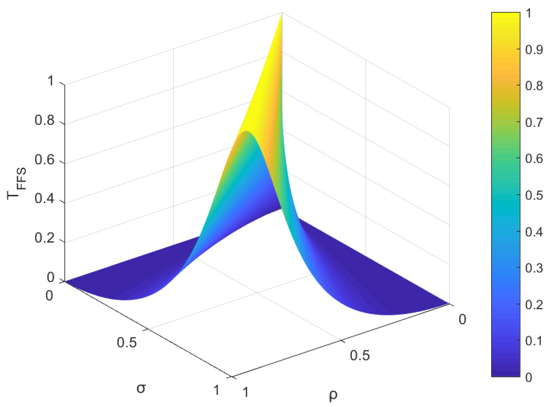
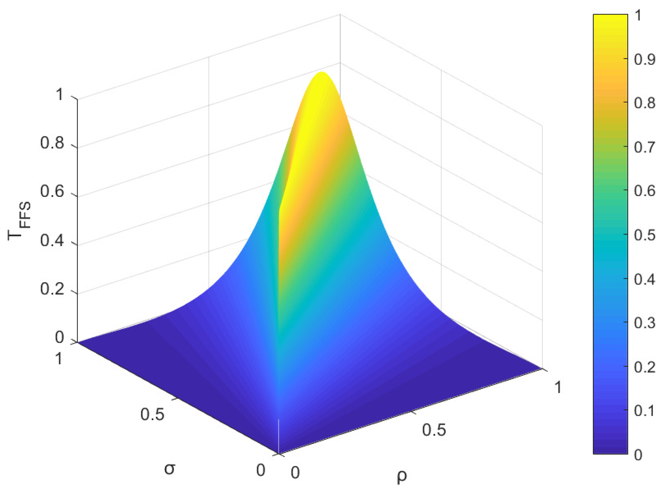
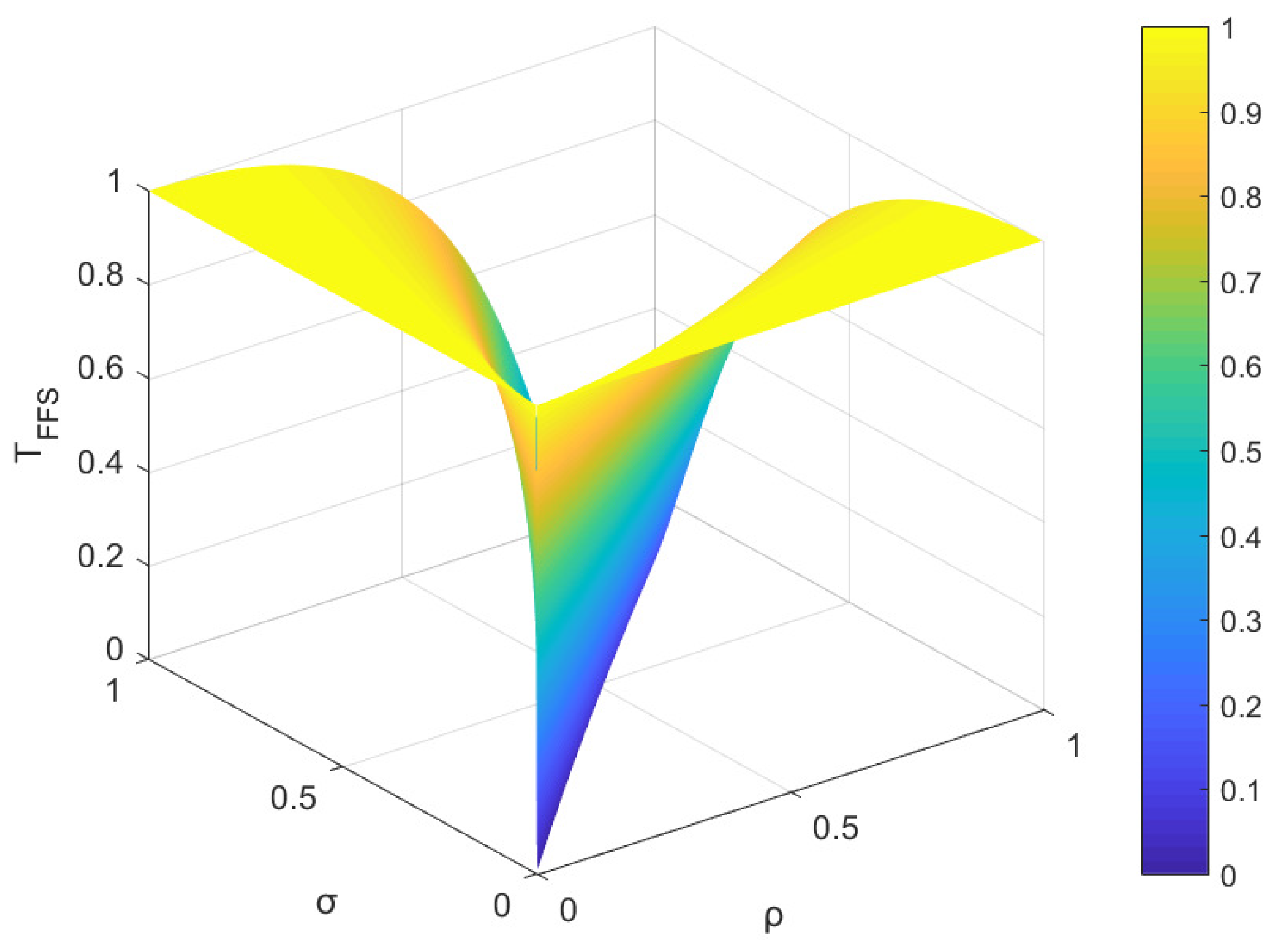
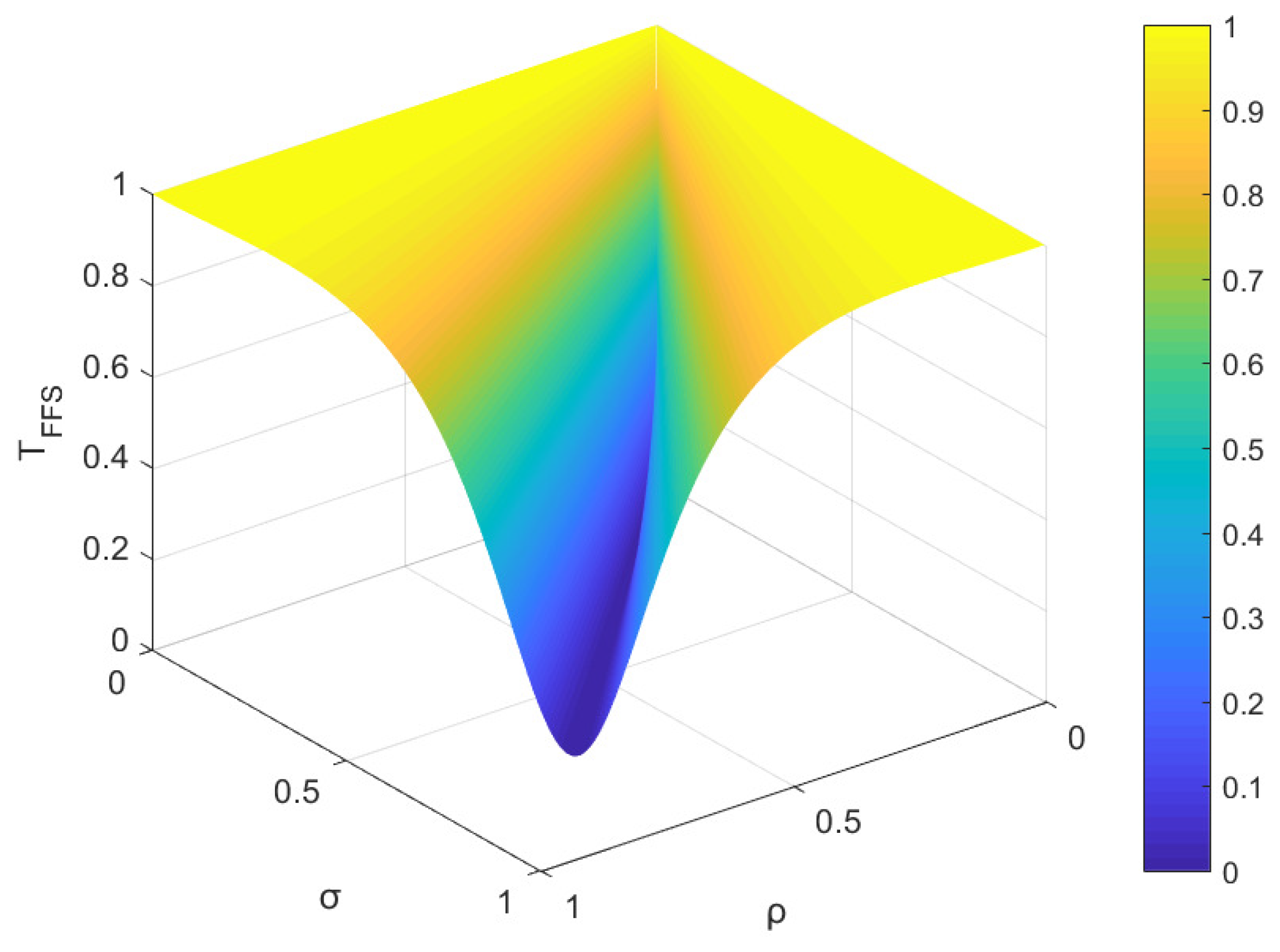
The FFSs

F_{1}

and

F_{2}

are found in Z, where

F_{1} = \{〈z, ρ, σ〉\}, F_{2} = \{〈z, σ, ρ〉\}

. In the present example, the parameters ρ and σ are utilized to denote the membership degree and non-membership degree of

F_{1}

and

F_{2}

, respectively. The values of ρ and σ fall within the interval

[0, 1]

, and these parameters satisfy condition

0 \leq ρ^{3} + σ^{3} \leq 1

. As per the proposed measure, Figure 1 and Figure 2, as well as Figure 3 and Figure 4, illustrate the trends of similarity and distance between

F_{1}

and

F_{2}

over a range of parameter values for ρ and σ, respectively.

Based on the observations from Figure 1 and Figure 2, it is evident that the similarity value and the distance value lie within the interval of [0, 1]. Notably, when ρ equals σ, the similarity measure between

F_{1}

and

F_{2}

attains its maximum value of 1, whereas when ρ equals 1 and σ equals 0 (or vice versa), the similarity measure reaches its minimum value of 0. As parameters ρ and σ vary within the range of [0, 1], the similarity measure changes correspondingly within the same range of [0, 1]. The change in distance measure is reversed. These results affirm that the Tanimoto similarity measures and the distance measures satisfy the boundedness Property (1) as defined in Definition 11 and Definition 15, respectively. The overall trend in Figure 1, Figure 2, Figure 3 and Figure 4 aligns with intuitive judgment, indicating that the Tanimoto measures meet the requirements of Property (1) in Definition 11 and Definition 15.

Example 3.

The three FFSs

F_{1}

and

F_{2}

found in Z, denoted as

F, G_{1}

and

G_{2}

, and shown in Table 5. It is evident from Table 5 that

G_{1} \neq G_{2}

, implying that the similarity between F and

G_{1}

s m (F, G_{1})

and the similarity between F and

G_{2}

s m (F, G_{2})

must be distinct. In Table 6, the outcomes of the Tanimoto similarity measures and those of the cosine similarity measure proposed by Kirişci [71] (indicated as

S_{F F S}^{1}

) are compared. Specifically, the Tanimoto similarity measures yield accurate outcomes that align with intuition. Nevertheless, the cosine similarity measure produces counter-intuitive outcomes and may fail to differentiate both FFSs correctly in practice. This highlights the superior precision of our proposed measures and the limitations of the cosine similarity measure. It can be concluded from this example that our proposed measures are more effective and superior to the cosine similarity measure.

Example 4.

There are some FFSs in

Z = \{z_{1}, z_{2}\}

, denoted as

F^{i}, G_{1}^{i}

and

G_{2}^{i}

(i = 1, 2, 3)

, and shown in Table 7, Table 8 and Table 9. It is evident from Table 7, Table 8 and Table 9 that

G_{1}^{i} \neq G_{2}^{i}

, implying that

s m (F^{i}, G_{1}^{i})

and

s m (F^{i}, G_{2}^{i})

must be distinct. In Table 10, Table 11 and Table 12, the outcomes of the Tanimoto similarity measures and those of the similarity measures proposed by Sahoo [72] (indicated as

S_{F F S}^{2}

S_{F F S}^{3}

S_{F F S}^{4}

S_{F F S}^{5}

and

S_{F F S}^{6}

) are compared. Specifically, the Tanimoto similarity measures yield accurate outcomes that align with intuition. Nevertheless, the similarity measures proposed by Sahoo produce counter-intuitive outcomes and may fail to differentiate both FFSs correctly in practice. This highlights the superior precision of our proposed similarity measures. It can be concluded from this example that our proposed measures are more effective and superior to the measures proposed by Sahoo.

Example 5.

There are three FFSs in

Z = \{z_{1}, z_{2}\}

, denoted as

F, G_{1}

and

G_{2}

, and shown in Table 13. It is evident from Table 13 that

G_{1} \neq G_{2}

, implying that the distance between F and

G_{1}

d m (F, G_{1})

and the similarity between F and

G_{2}

d m (F, G_{2})

must be distinct. In Table 14, the outcomes of the Tanimoto distance measures and those of the Hellinger distance measure and the triangular distance measure proposed by Deng [70] (indicated as

d_{H}

and

d_{T}

) are compared. Specifically, the Tanimoto distance measures yield accurate outcomes that align with intuition. Nevertheless, the other distance measures produce counter-intuitive outcomes and may fail to differentiate both FFSs correctly in practice. It can be concluded from this example that our proposed measures are more effective and superior to the Hellinger distance measure and the triangular distance measure.

Example 6.

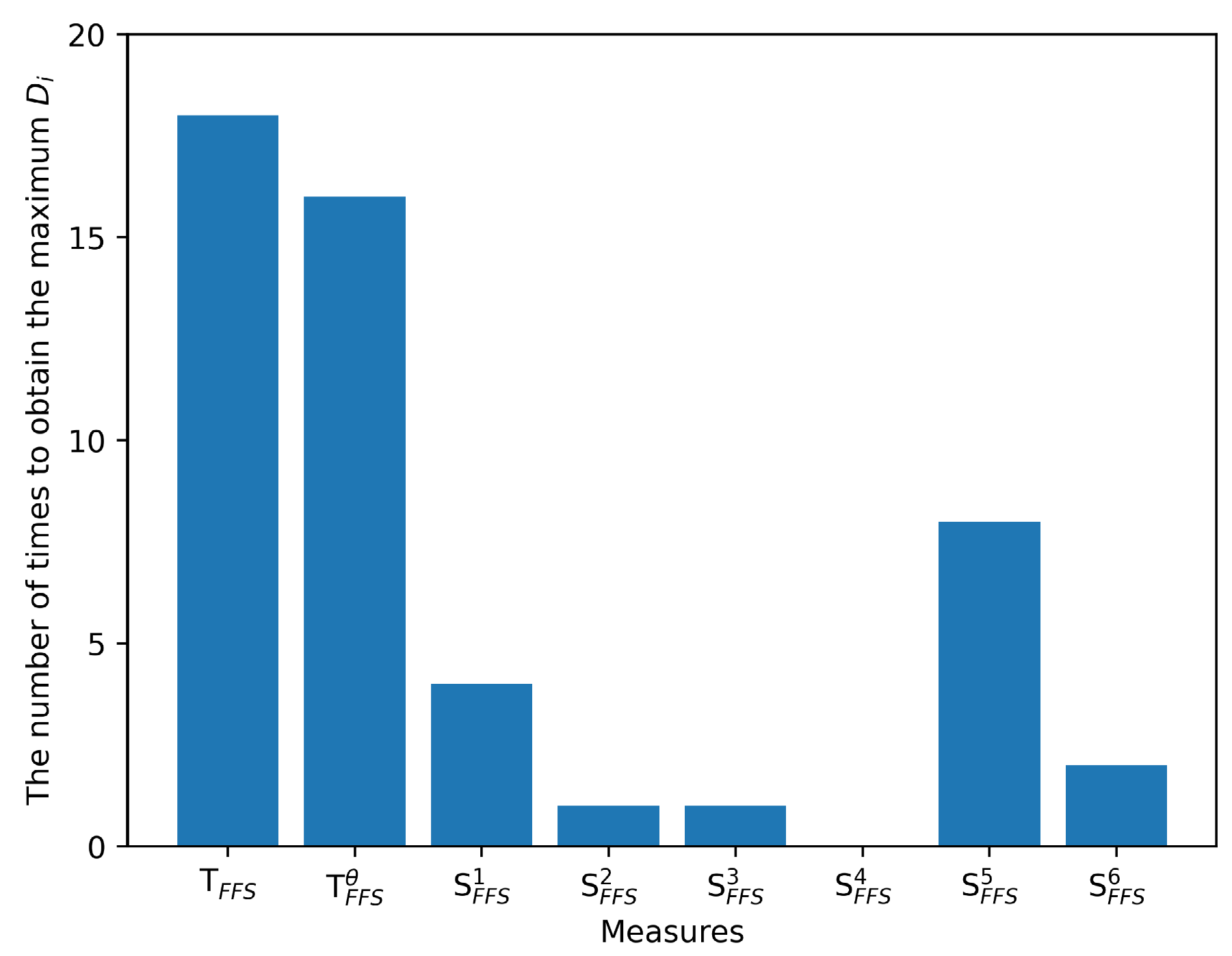
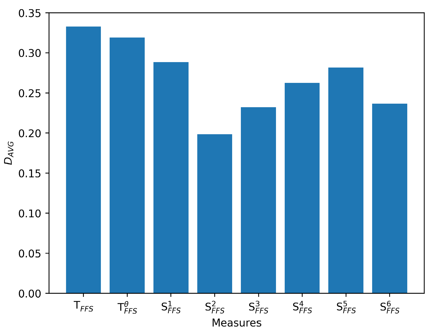
A_{i}

B_{i}

and

C_{i}

are three randomly generated FFSs under case

i (i = 1, 2, \dots, 50)

. Now we use the proposed similarity measures to measure their similarity and get a difference by subtracting the minimum value from the maximum value of the obtained results, denoted as

D_{i}

. We conducted 50 such experiments and averaged the final results to obtain the average difference between the maximum and minimum values of the similarity results in these 50 experiments, denoted as

D_{A V G}

. Specifically, the

D_{i}

and

D_{A V G}

for FFSs can be calculated as follow:

D_{i} = max (T_{F F S} (A_{i}, B_{i}), T_{F F S} (A_{i}, C_{i}), T_{F F S} (B_{i}, C_{i}))

(31)

D_{A V G} = \frac{1}{50} \sum_{i = 1}^{50} D_{i}

(32)

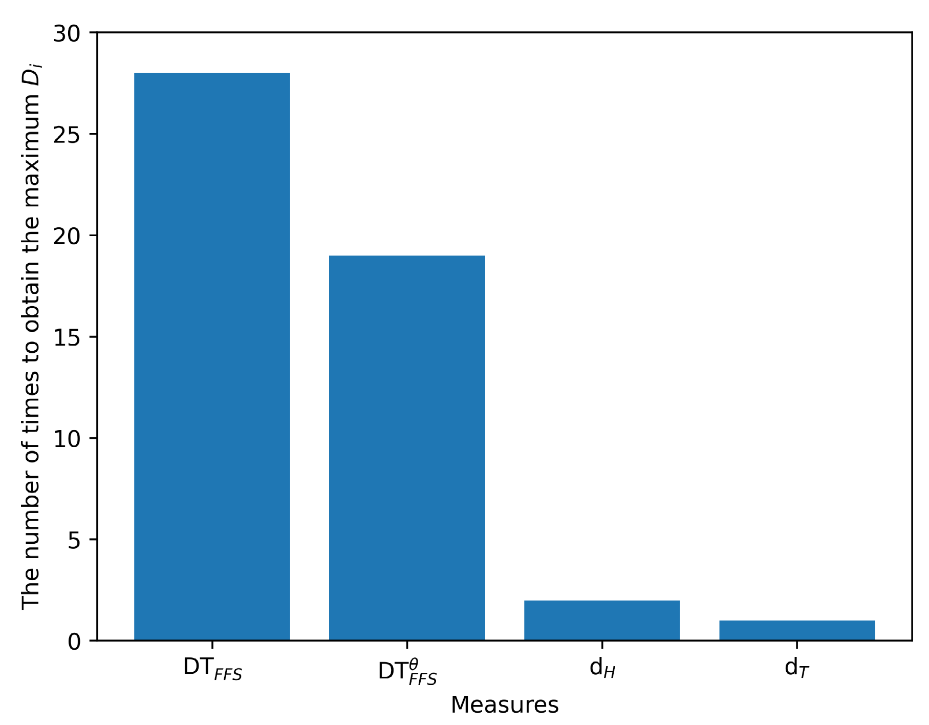
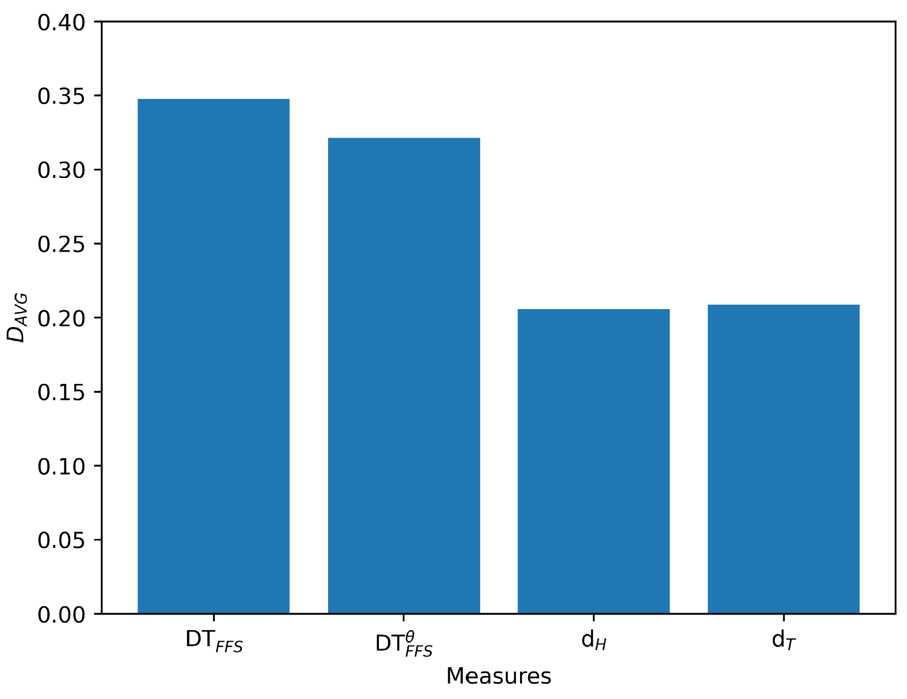
. Similarly, we compare the

D_{i}

s and

D_{A V G}

s obtained using other measures. Figure 5 presents the frequency of different similarity measures attaining the maximum

D_{i}

in these 50 experiments, while Figure 6 depicts the

D_{A V G}

s of different similarity measures across these 50 experiments. We conducted the same experiment using distance measures and the results are presented in Figure 7 and Figure 8.

Figure 5 illustrates that the Tanimoto similarity measures tend to maximize differences of the similarity between different FFSs while Figure 6 illustrates that the Tanimoto similarity reveals that they produce the maximum average differences between the maximum and minimum similarity values. These findings suggest that our proposed similarity measures generate similarity scores with greater variation, thereby endowing the Tanimoto similarity measures with greater ability to discern differences across various levels of FFSs. Furthermore, it can exhibit better performance in discriminating FFSs with high similarity. The heightened differences in similarity scores assigned to different FFSs can bolster the trustworthiness of FFSs classification and facilitate more confident decision-making. However, S1 and S2 exhibit the smaller values of in Figure 5 and Figure 6, indicating a tendency to assign similar values to diverse samples, potentially resulting in greater hesitation when making decisions within the same environment, thereby impeding efficient and confident decision-making. These outcomes underscore the superiority of our proposed similarity measures over the extant ones under scrutiny. Similarly, we performed the identical analysis on distance measures and achieved the same outcomes, as depicted in Figure 7 and Figure 8, corroborating the superiority of our proposed distance measures. These properties will be further demonstrated by additional instances in the future examples.

4. Applications

This section presents two models that are designed to tackle pattern recognition, medical diagnosis and MADM based on the proposed measures. To substantiate the efficiency of the proposed models, a series of experiments comparing with the existing measures were conducted.

4.1. A novel model for pattern recognition and medical diagnosis

Given a set of attributes

Z = {z_{1}, z_{2}, \dots, z_{n}}

, we aim to classify the test samples

S = {S_{1}, S_{2}, \dots, S_{m}}

based on k patterns

F = {F_{1}, F_{2}, \dots, F_{k}}

. The patterns are represented by FFSs, denoted as

F_{i} = {〈z_{l}, ρ_{F_{i}}, σ_{F_{i}}〉 : z_{l} \in Z} (i = 1, 2, \dots, k)

, while the test samples are expressed as FFSs, denoted as

S_{j} = {〈z_{l}, ρ_{S_{j}}, σ_{S_{j}}〉 : z_{l} \in Z} (j = 1, 2, \dots, m)

. Our objective is to accurately classify the test samples according to the given patterns. The recognition process is outlined below:

Step 1: Calculate the Tanimoto similarity(or distance) between $S_{j} (j = 1, 2, \dots, m)$ and

$F_{i} (i = 1, 2, \dots, k)$ .
Step 2: Obtain the maximum Tanimoto similarity $s (F_{o}, S_{j})$ using equation 35 or the minimum Tanimoto distance $d (F_{o}, S_{j})$ using equation 36:

$s (F_{o}, S_{j}) = max {T_{F F S} (F_{i}, S_{j})}$

(33)

$d (F_{o}, S_{j}) = min {D T_{F F S} (F_{i}, S_{j})}$

(34)
Step 3: If any pattern $F_{o}$ has the highest Tanimoto similarity between $S_{i}$ , then, $S_{i}$ and $F_{o}$ belong to the same category:

$o = arg max {s (F_{o}, S_{j})}, S_{j} \to F_{o}$

(35)

If distance measure is used as the standard of measure, then the following form would be applied:

$o = arg min {d (F_{o}, S_{j})}, S_{j} \to F_{o}$

(36)

Example 7

([70]). This example pertains to the pattern recognition of unknown samples, where three known sample categories are represented by FFS

F_{i} (i = 1, 2, 3)

and the universe of discourse consists of their attributes

z_{i} (i = 1, 2, 3)

. Specifically,

\begin{matrix} F_{1} = {〈z_{1}, 0.8, 0.3〉, 〈z_{2}, 0.7, 0.2〉, 〈z_{3}, 0.6, 0.4〉}, \\ F_{2} = {〈z_{1}, 0.9, 0.2〉, 〈z_{2}, 1.0, 0.0〉, 〈z_{3}, 0.8, 0.1〉}, \\ F_{3} = {〈z_{1}, 0.2, 0.7〉, 〈z_{2}, 0.4, 0.6〉, 〈z_{3}, 0.7, 0.5〉} . \end{matrix}

There exists a sample S with unknown category, defined as:

S = {〈z_{1}, 0.8, 0.1〉, 〈z_{2}, 0.9, 0.3〉, 〈z_{3}, 0.9, 0.0〉},

and the proposed Tanimoto measures are employed to determine the category of the unknown sample S. The recognition process is as follows:

Step 1: Calculate the Tanimoto similarity(or distance) between $F_{i} (i = 1, 2, 3)$ and S:

$\begin{matrix} T_{F F S} (F_{1}, S) = 0.665 \\ T_{F F S} (F_{1}, S) = 0.894 \\ T_{F F S} (F_{1}, S) = 0.238 \\ D T_{F F S} (F_{1}, S) = 0.335 \\ D T_{F F S} (F_{1}, S) = 0.106 \\ D T_{F F S} (F_{1}, S) = 0.762 \end{matrix}$
Step 2: Obtain the maximum Tanimoto similarity $s (F_{o}, S_{j})$ using equation 35 or the minimum Tanimoto distance $d (F_{o}, S_{j})$ using equation 36:

$\begin{matrix} s (F_{2}, S) = 0.894 \\ d (F_{2}, S) = 0.1055 \end{matrix}$
Step 3: According to the equation 37 or equation 38, S and $F_{2}$ belongs to the same pattern.

A comparative analysis is conducted with the results obtained by the existing similarity measures and distance measures mentioned in Section 2. The results are presented in Table 15 and Table 16.

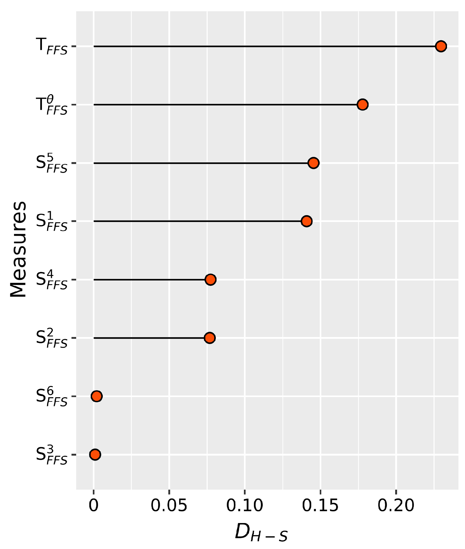
Based on the principle of minimum distance, it was determined that sample S is most similar to sample

F_{2}

, which is consistent with the findings in reference [70]. It is worth noting that other distance measures have also produced similar recognition results. Furthermore, based on the principle of maximum similarity, similarity measures

S_{F F S}^{1}

S_{F F S}^{4}

S_{F F S}^{5}

and

S_{F F S}^{6}

yielded the same recognition results, classifying sample S into

F_{2}

. Conversely, the results of

S_{F F S}^{2}

and

S_{F F S}^{3}

are different, as they classify sample S as

F_{1}

. Therefore, the accuracy of

S_{F F S}^{2}

and

S_{F F S}^{3}

remains to be discussed. These findings effectively demonstrates the efficacy of our proposed Tanimoto similarity measures and distance measures. Moreover, the difference between the highest similarity scores and second-highest similarity scores for each similarity measure was calculated which are record as

D_{H - S}

s. For instance, the

D_{H - S}

for

T_{F F S}

in this example can be calculated as

D_{H - S} = 0.894 - 0.238 = 0.656

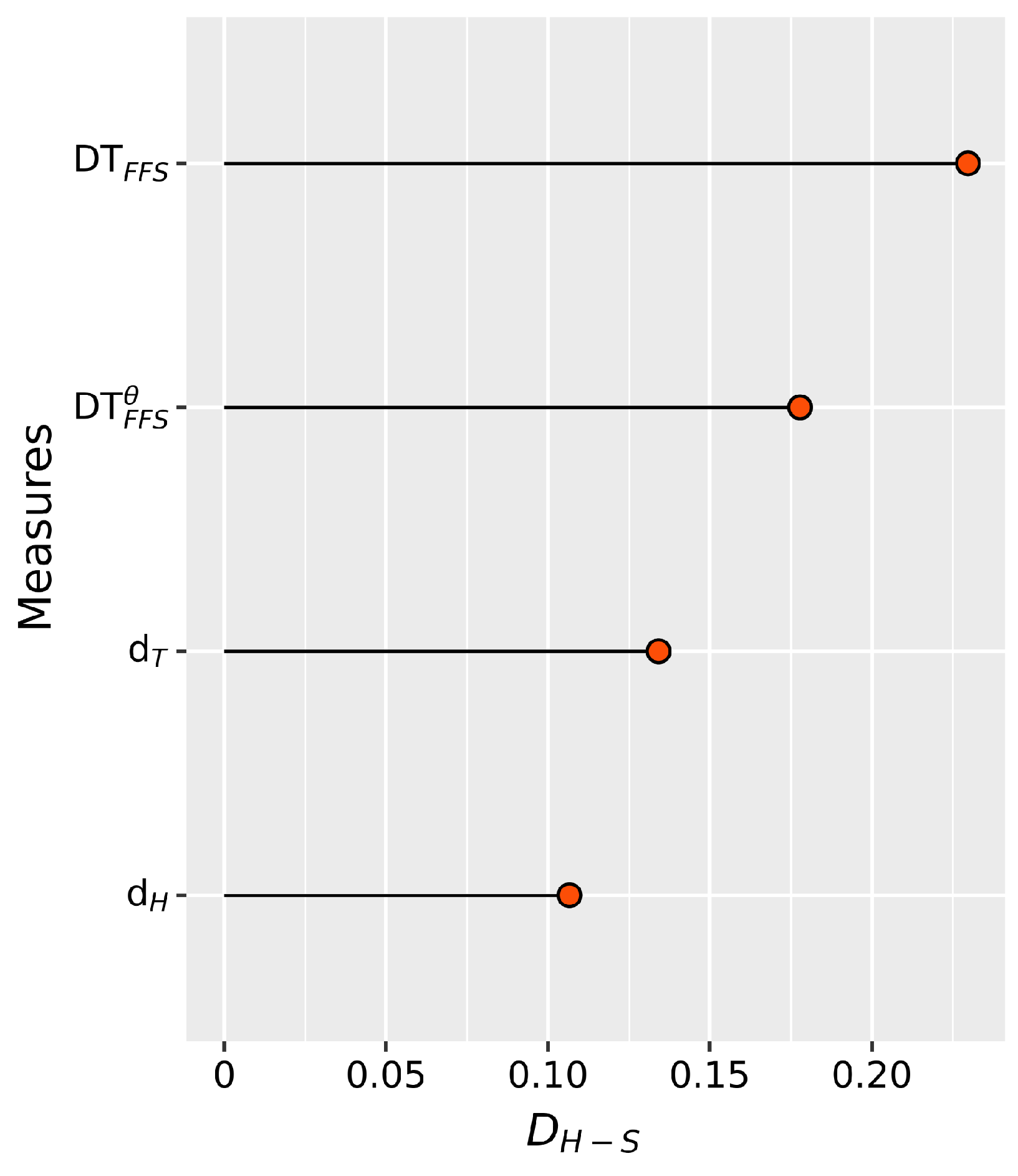
. The

D_{H - S}

s for the other similarity measures are shown in Figure 9. The results of Tanimoto similarity measure show the largest difference between the highest and second-highest similarity scores, ranking second when considering hesitation. The similarity values between S and

F_{2}

, as determined via our proposed similarity measures, are noticeably distinct from those between S and other FFSs. Thus, we can confidently assert that

F_{2}

is a more appropriate choice. However, the similarity values between S and known samples obtained from other similarity measures are more close to each other. Therefore, making decisions based on these similarity measures may lead to greater hesitation. Similarly, we performed the same operation on distance measurement, the

D_{H - S}

s for each distance measure are calculated and are shown in Figure 10. The results of Tanimoto distance measure show the largest difference between the highest and second-highest similarity scores, ranking second when considering hesitation. Therefore, we can obtain the same superiority conclusion as similarity measures above. These results reinforce the conclusion derived in Example 6, indicating that our proposed similarity measures and distance measures excel in differentiating between samples displaying high levels of similarity.

Example 8.

This example is the pattern recognition of mineral categories. Suppose that there are five typical mixed minerals represented by FFS

F_{i} (i = 1, 2, 3, 4, 5)

, and each mineral is composed of six basic minerals which form the universe of discourse

z_{i} (i = 1, 2, 3, 4, 5, 6)

. Our objective is to use the proposed measures to identify the category to which an unknown mixed mineral S belongs. Table ref tab7 shows the known FFSs and unknown S, while Table 18 and Table 19 summarize the results obtained from similarity and distance measures, respectively.

Table 18 reveals that the Tanimoto similarity of mineral S and

F_{4}

is the highest, suggesting that mineral S belongs to

F_{4}

. This is consistent with the results of other similarity measures. In addition, Table 19 shows that the Tanimoto distance between S and

F_{4}

is the smallest, indicating that mineral S is the closest to

F_{4}

. These findings align with the results obtained from other distance measures. The results of our experiments provide evidence for the effectiveness of the proposed measures.

Example 9

([75]). Assuming the presence of four patients, namely Ragu, Mathi, Velu, and Karthi, denoted by

I = {I_{1}, I_{2}, I_{3}, I_{4}}

, and exhibiting symptoms including Headache, Acidity, Burning eyes, Back pain, and Depression, represented as

Z = {Z_{1}, Z_{2}, Z_{3}, Z_{4}, Z_{5}}

. The set of possible diagnoses is denoted by

D = {D_{1}, D_{2}, D_{3}, D_{4}, D_{5}}

, and includes:

D_{1}

: Stress;

D_{2}

: Ulcer;

D_{3}

: Vision problem;

D_{4}

: Spinal problem;

D_{5}

: Blood pressure. The relation

I \to Z

is expressed by FFSs, as shown in Table 20, while the relation

Z \to D

is represented by FFSs and listed in Table 21. Every entry in both tables is defined by the FFS, with the values indicating membership degree and non-membership degree, respectively. The proposed similarity and distance measures are employed to evaluate the similarity and distance between each patient and potential diagnosis. Based on the principle of maximum similarity or minimum distance, each patient is diagnosed accordingly. Table 22, Table 23, and Table 24 present the similarity measure outcomes and distance of patient I towards each diagnosis D, alongside the ultimate diagnosis results.

Based on the findings presented in Table 22 and Table 23, it is observed that

I_{1}

exhibits the highest Tanimoto similarity measure and the smallest Tanimoto distance measure towards

D_{1}

;

I_{2}

displays the highest Tanimoto similarity measure and the smallest Tanimoto distance measure towards

D_{4}

;

I_{3}

demonstrates the highest Tanimoto similarity measure and the smallest Tanimoto distance measure towards

D_{3}

; and

I_{4}

showcases the highest Tanimoto similarity measure and the smallest Tanimoto distance measure towards

D_{1}

. Thus, we can conclude that Ragu is diagnosed with stress, Mathi with spinal problems, Velu with vision problems, and Karthi with stress.

In order to validate the effectiveness of our proposed measures, a comparative analysis was performed against other techniques, and the outcomes have been summarized in Table 24. It is observed from Table 24 that our proposed measures provide diagnostic outcomes that are consistent with those obtained using Xiao and Ding’s method [75], and Deng’s method [70] indicating the potential of our measures to address the medical diagnosis problem. The experimental results lend support to the practicability of our proposed similarity and distance measures.

4.2. A novel model for MADM

Suppose that

I = {I_{1}, I_{2} \dots, I_{m}}

is a discrete set of alternatives, and

A = {A_{1}, A_{2} \dots, A_{n}}

is the set of attributes,

ω = {ω_{1}, ω_{2} \dots, ω_{n}}

is the weighting vector of the attribute

A_{j} (j = 1, 2, \dots, n)

, where

ω > 0

\sum_{j = 1}^{n} w_{j} = 1

. Suppose that

R = {(ρ_{i j}, σ_{i j})}_{m \times n}

is the Fermaten fuzzy matrix, where

ρ_{i j}

indicates the degree that the alternative

I_{i}

satisfies the attribute

A_{j}

and

σ_{i j}

indicates the degree that the alternative

I_{i}

does not satisfy the attribute

A_{j}

ρ_{i j} \subset [0, 1]

σ_{i j} \subset [0, 1]

{(ρ_{i j})}^{3} + {(σ_{i j})}^{3} \leq 1

i = 1, 2, \dots, m

j = 1, 2, \dots, n

. The proposed model is described below:

Step 1:: Defining the Fermatean fuzzy positive ideal solution $I^{+}$ :

$(ρ^{+}, σ^{+}) = ((ρ_{1}^{+}, σ_{1}^{+}), (ρ_{2}^{+}, σ_{2}^{+}), \dots, (ρ_{j}^{+}, σ_{j}^{+})) = ((1, 0), (1, 0), \dots (1, 0))$

(37)

When an attribute $A_{j}$ is a negative influence, we define the positive ideal solution as $(0, 1)$ .
Step 2:: Calculating the weighted Tanimoto similarity measures(or the Tanimoto distance measures) between $I_{i} (i = 1, 2, \dots, m)$ and $I^{+}$ as follows:

$T_{F F S}^{ω} (I_{i}, I^{+}) = \sum_{i = 1}^{n} \frac{ω_{i} (ρ_{i j}^{3} {(ρ_{j}^{+})}^{3} + σ_{i j}^{3} {(σ_{j}^{+})}^{3})}{ρ_{i j}^{6} + σ_{i j}^{6} + {(ρ_{j}^{+})}^{6} + {(σ_{j}^{+})}^{6} - ρ_{i j}^{3} {(ρ_{j}^{+})}^{3} - σ_{i j}^{3} {(σ_{j}^{+})}^{3}}$

(38)

$T_{F F S}^{θ ω} (I_{i}, I^{+}) = \sum_{i = 1}^{n} \frac{ω_{i} (ρ_{i j}^{3} {(ρ_{j}^{+})}^{3} + σ_{i j}^{3} {(σ_{j}^{+})}^{3} + θ_{i j}^{3} {(θ_{j}^{+})}^{3})}{ρ_{i j}^{6} + σ_{i j}^{6} + θ_{i j}^{6} + {(ρ_{j}^{+})}^{6} + {(σ_{j}^{+})}^{6} + {(θ_{j}^{+})}^{6} - ρ_{i j}^{3} {(ρ_{j}^{+})}^{3} - σ_{i j}^{3} {(σ_{j}^{+})}^{3} - θ_{i j}^{3} {(θ_{j}^{+})}^{3}}$

(39)

or

$D T_{F F S}^{ω} (I_{i}, I^{+}) = 1 - \sum_{i = 1}^{n} \frac{ω_{i} (ρ_{i j}^{3} {(ρ_{j}^{+})}^{3} + σ_{i j}^{3} {(σ_{j}^{+})}^{3})}{ρ_{i j}^{6} + σ_{i j}^{6} + {(ρ_{j}^{+})}^{6} + {(σ_{j}^{+})}^{6} - ρ_{i j}^{3} {(ρ_{j}^{+})}^{3} - σ_{i j}^{3} {(σ_{j}^{+})}^{3}}$

(40)

$D T_{F F S}^{θ ω} (I_{i}, I^{+}) = 1 - \sum_{i = 1}^{n} \frac{ω_{i} (ρ_{i j}^{3} {(ρ_{j}^{+})}^{3} + σ_{i j}^{3} {(σ_{j}^{+})}^{3})}{ρ_{i j}^{6} + σ_{i j}^{6} + {(ρ_{j}^{+})}^{6} + {(σ_{j}^{+})}^{6} - ρ_{i j}^{3} {(ρ_{j}^{+})}^{3} - σ_{i j}^{3} {(σ_{j}^{+})}^{3}}$

(41)
Step 3:: Rank all the alternatives $I_{i} (i = 1, 2, \dots, m)$ and select the best one(s) in accordance with the weighted Tanimoto similarity measures or the weighted Tanimoto distance measures. If a alternative exhibits a higher weighted Tanimoto similarity or the smaller weighted Tanimoto distance, it is a more important alternative. If any alternative has the highest weighted Tanimoto similarity value or the smallest Tanimoto distance value, then, it is the most important alternative.

Example 10.

A certain company intends to procure a set of computers from a pool of five alternative model options, denoted as

I_{i} (i = 1, 2, 3, 4, 5)

. The company has identified four crucial attributes for selection, namely, manufacturing materials, response speed, service life, and after-sales quality

A_{j} (j = 1, 2, 3, 4, 5)

. These attributes are assigned weights, denoted as

ω_{j} (j = 1, 2, 3, 4)

), where

ω = (0.4, 0.1, 0.2, 0.3)

, which together form the Fermatean fuzzy decision matrix R:

R = [\begin{matrix} (0.6089, 0.5983) & (0.6236, 0.3782) & (0.3024, 0.3979) & (0.4229, 0.2788) \\ (0.7098, 0.2052) & (0.7238, 0.3782) & (0.6089, 0.2052) & (0.7238, 0.3782) \\ (0.1950, 0.7008) & (0.3224, 0.5780) & (0.4057, 0.5983) & (0.1189, 0.4780) \\ (0.6720, 0.5592) & (0.2213, 0.4780) & (0.4057, 0.4974) & (0.6236, 0.4780) \\ (0.3024, 0.2999) & (0.2213, 0.4780) & (0.5076, 0.2052) & (0.3224, 0.2788) \end{matrix}]

. We propose the use of the MADM model to identify the most suitable solution.

Step 1:: Defining the Fermatean fuzzy positive ideal solution $I^{+}$ :

$\begin{matrix} (ρ^{+}, σ^{+}) & = ((ρ_{1}^{+}, σ_{1}^{+}), (ρ_{2}^{+}, σ_{2}^{+}), (ρ_{3}^{+}, σ_{3}^{+}), (ρ_{4}^{+}, σ_{4}^{+})) \\ = ((1, 0), (1, 0), (1, 0), (1, 0)) . \end{matrix}$

Here, all attributes are considered positive attributes, so they are defined as (1, 0)
Step 2:: Calculating the weighted Tanimoto measures between $I_{i} (i = 1, 2, \dots, m)$ and $I^{+}$ as Table 25 and Table 26:
Step 3:: We can find that the weighted similarity between $I_{2}$ and $I^{+}$ is the highest, similarly, the weighted distance between $I_{2}$ and $I^{+}$ is the smallest, so we choose $I_{2}$ the best alternative.

Furthermore, we gained the same selection result by the TOPSIS method proposed by Murat [71], and the calculation results are shown in Table 27. The closeness index γ and the positive ideal solution obtained by Murat

U^{+}

are utilized in this study. As the γ gets smaller,

I_{2}

is taken as the best alternative.

Example 11.

At present, there are five students

I_{i} (i = 1, 2, 3, 4, 5)

available, from whom a certain company needs to select two interns. A set of selection criteria

A_{j} (j = 1, 2, 3, 4, 5)

has been developed, which considers the students’ academic performance, competition participation, school activities, mastery of professional knowledge related to the position and violations of discipline on campus. However, violations of discipline on campus are not considered positive attributes. Weights

ω = (0.4, 0.2, 0.1, 0.2, 0.1)

have been assigned to each attribute, resulting in the formation of a Fermatean fuzzy decision matrix R:

R = [\begin{matrix} (0.471, 0.939) & (0.806, 0.269) & (0.132, 0.819) & (0.348, 0.977) & (0.547, 0.297) \\ (0.227, 0.538) & (0.181, 0.403) & (0.119, 0.125) & (0.440, 0.387) & (0.469, 0.383) \\ (0.332, 0.204) & (0.646, 0.356) & (0.779, 0.375) & (0.457, 0.400) & (0.941, 0.124) \\ (0.850, 0.121) & (0.974, 0.195) & (0.512, 0.904) & (0.653, 0.048) & (0.605, 0.273) \\ (0.900, 0.037) & (0.19, 0.148) & (0.221, 0.607) & (0.576, 0.039) & (0.881, 0.321) \end{matrix}]

. The proposed MDAM model is being utilized for selecting the most suitable interns:

Step 1:: Defining the Fermatean fuzzy positive ideal solution $I^{+}$ :

$\begin{matrix} (ρ^{+}, σ^{+}) & = ((ρ_{1}^{+}, σ_{1}^{+}), (ρ_{2}^{+}, σ_{2}^{+}), (ρ_{3}^{+}, σ_{3}^{+}), (ρ_{4}^{+}, σ_{4}^{+})), (ρ_{5}^{+}, σ_{5}^{+}) \\ = ((1, 0), (1, 0), (1, 0), (1, 0), (0, 1)) . \end{matrix}$

(43)

Here, campus disciplinary behavior is not considered a positive factor and is therefore defined as (0, 1).
Step 2:: Calculating the weighted Tanimoto measures between $I_{i} (i = 1, 2, \dots, m)$ and $I^{+}$ as Table 28 and Table 29:
Step 3:: Table 30 presents the sorted similarity measures and distance measures based on the obtained data, in accordance with the principles of maximum similarity and minimum distance. Based on the principles of maximum similarity and minimum distance, we choose $I_{4}$ and $I_{5}$ as the optimal choices.

5. Conclusion

Fermatean fuzzy sets (FFSs) are an effective tool for representing uncertain information. However, the accurate measure of similarity and distance between two FFSs remains a long-term research problem. In this paper, we propose several new similarity and distance measures for FFSs based on the Tanimoto similarity concept. Numerical experiments demonstrate that the proposed measures not only avoid the counter-intuitive situations of many existing measures but also obtain more obvious results in distinguishing FFSs. Compared with some existing FFSs measures, the proposed measures are more effective and superior. We also applied our proposed measures to pattern recognition, medical diagnosis, and multiple-attribute decision-making tasks in Fermatean fuzzy environments, and obtained effective and reasonable results.Therefore, it can be easily used to measure feature similarity and support decision-making processes in complex and uncertain scenarios. In our future research, we plan to explore the full potential of our proposed similarity and distance measures by applying it to various problems in Fermatean fuzzy environments. By doing so, we aim to enhance its impact and validate its effectiveness in real-life scenarios. This will demonstrate its capability in providing practical solutions for complex and uncertain problems.

Author Contributions

Conceptualization, H.W.; Methodology, H.W.; Software, G.F.; Investigation, H.W.; Data curation, C.T.; Writing—original draft, H.W.; Writing—review & editing, C.L.; Project administration, C.L. All authors have read and agreed to the published version of the manuscript.

Funding

This research was funded by National Natural Science Foundation of China grant number 62102235 and Natural Science Foundation of Shandong Province grant number ZR2020QF029.

Data Availability Statement

Both data and algorithms are listed in the article.

Conflicts of Interest

The authors declare no conflict of interest.

References

Yager, R.R. On using the Shapley value to approximate the Choquet integral in cases of uncertain arguments. IEEE Transactions on Fuzzy Systems 2017, 26, 1303–1310. [Google Scholar] [CrossRef]
Wang, X.; Song, Y. Uncertainty measure in evidence theory with its applications. Applied Intelligence 2018, 48, 1672–1688. [Google Scholar] [CrossRef]
Hariri, R.H.; Fredericks, E.M.; Bowers, K.M. Uncertainty in big data analytics: survey, opportunities, and challenges. Journal of Big Data 2019, 6, 1–16. [Google Scholar] [CrossRef]
Zadeh, L.A. Fuzzy sets. Information & Control 1965, 8, 338–353. [Google Scholar]
Zadeh, L.A. Fuzzy sets as a basis for a theory of possibility. Fuzzy Sets and Systems 1978, 1, 3–28. [Google Scholar] [CrossRef]
Torra, V. Hesitant fuzzy sets. International Journal of Intelligent Systems 2010, 25, 529–539. [Google Scholar] [CrossRef]
Hung, W.L.; Yang, M.S. Fuzzy entropy on intuitionistic fuzzy sets. International Journal of Intelligent Systems 2010, 21, 443–451. [Google Scholar] [CrossRef]
Pawlak, Z. Rough sets. International Journal of Computer & Information Sciences 1982, 11, 341–356. [Google Scholar]
Deng, Y. Uncertainty measure in evidence theory. Science China Information Sciences 2020, 63, 210201. [Google Scholar] [CrossRef]
Kabir, S.; Papadopoulos, Y. A review of applications of fuzzy sets to safety and reliability engineering. International Journal of Approximate Reasoning 2018, 100, 29–55. [Google Scholar] [CrossRef]
Thong, N.T.; others. HIFCF: An effective hybrid model between picture fuzzy clustering and intuitionistic fuzzy recommender systems for medical diagnosis. Expert Systems with Applications 2015, 42, 3682–3701. [Google Scholar] [CrossRef]
Haseli, G.; Sheikh, R.; Wang, J.; Tomaskova, H.; Tirkolaee, E.B. A novel approach for group decision making based on the best–worst method (G-bwm): Application to supply chain management. Mathematics 2021, 9, 1881. [Google Scholar] [CrossRef]
Ma, Z.; Liu, Z.; Luo, C.; Song, L. Evidential classification of incomplete instance based on K-nearest centroid neighbor. Journal of Intelligent & Fuzzy Systems 2021, 41, 7101–7115. [Google Scholar]
Mardani, A.; Hooker, R.E.; Ozkul, S.; Yifan, S.; Nilashi, M.; Sabzi, H.Z.; Fei, G.C. Application of decision making and fuzzy sets theory to evaluate the healthcare and medical problems: a review of three decades of research with recent developments. Expert Systems with Applications 2019, 137, 202–231. [Google Scholar] [CrossRef]
Hwang, G.J.; Tu, Y.F. Roles and research trends of artificial intelligence in mathematics education: A bibliometric mapping analysis and systematic review. Mathematics 2021, 9, 584. [Google Scholar] [CrossRef]
Atanassov, K.T. Intuitionistic fuzzy sets. Fuzzy Sets & Systems 1986, 20, 87–96. [Google Scholar]
Shafer, G. A mathematical theory of evidence; Vol. 42, Princeton University Press, 1976.
Wang, G. Rough reduction in algebra view and information view. International Journal of Intelligent Systems 2003, 18, 679–688. [Google Scholar] [CrossRef]
Alcantud, J.C.R.; Khameneh, A.Z.; Kilicman, A. Aggregation of infinite chains of intuitionistic fuzzy sets and their application to choices with temporal intuitionistic fuzzy information. Information Sciences 2020, 514, 106–117. [Google Scholar] [CrossRef]
Balasubramaniam, P.; Ananthi, V. Image fusion using intuitionistic fuzzy sets. Information Fusion 2014, 20, 21–30. [Google Scholar] [CrossRef]
Ngan, R.T.; Ali, M.; Fujita, H.; Abdel-Basset, M.; Giang, N.L.; Manogaran, G.; Priyan, M.; others. A new representation of intuitionistic fuzzy systems and their applications in critical decision making. IEEE Intelligent Systems 2019, 35, 6–17. [Google Scholar]
Yager, R.R. Pythagorean fuzzy subsets. 2013 joint IFSA world congress and NAFIPS annual meeting (IFSA/NAFIPS). IEEE, 2013, pp. 57–61.
Premalatha, R.; Dhanalakshmi, P. Enhancement and segmentation of medical images through Pythagorean fuzzy sets-An innovative approach. Neural Computing and Applications 2022, 34, 11553–11569. [Google Scholar] [CrossRef]
Naeem, K.; Riaz, M.; Karaaslan, F. Some novel features of Pythagorean m-polar fuzzy sets with applications. Complex & Intelligent Systems 2021, 7, 459–475. [Google Scholar]
Li, L.; Zhang, R.; Wang, J.; Zhu, X.; Xing, Y. Pythagorean fuzzy power Muirhead mean operators with their application to multi-attribute decision making. Journal of Intelligent & Fuzzy Systems 2018, 35, 2035–2050. [Google Scholar]
Senapati, T.; Yager, R.R. Fermatean fuzzy sets. Journal of Ambient Intelligence and Humanized Computing 2019, 11, 663–674. [Google Scholar] [CrossRef]
Keshavarz-Ghorabaee, M.; Amiri, M.; Hashemi-Tabatabaei, M.; Zavadskas, E.K.; Kaklauskas, A. A new decision-making approach based on Fermatean fuzzy sets and WASPAS for green construction supplier evaluation. Mathematics 2020, 8, 2202. [Google Scholar] [CrossRef]
Garg, H.; Shahzadi, G.; Akram, M. Decision-making analysis based on Fermatean fuzzy Yager aggregation operators with application in COVID-19 testing facility. Mathematical Problems in Engineering 2020, 2020, 1–16. [Google Scholar] [CrossRef]
Aydemir, S.B.; Yilmaz Gunduz, S. Fermatean fuzzy TOPSIS method with Dombi aggregation operators and its application in multi-criteria decision making. Journal of Intelligent & Fuzzy Systems 2020, 39, 851–869. [Google Scholar]
Shahzadi, G.; Akram, M. Group decision-making for the selection of an antivirus mask under fermatean fuzzy soft information. Journal of Intelligent & Fuzzy Systems 2021, 40, 1401–1416. [Google Scholar]
Gul, M.; Lo, H.W.; Yucesan, M. Fermatean fuzzy TOPSIS-based approach for occupational risk assessment in manufacturing. Complex & Intelligent Systems 2021, 7, 2635–2653. [Google Scholar]
Sergi, D.; Sari, I.U. Fuzzy capital budgeting using fermatean fuzzy sets. In Intelligent and Fuzzy Techniques: Smart and Innovative Solutions: Proceedings of the INFUS 2020 Conference, Istanbul, Turkey, July 21-23, 2020; Springer, 2021; pp. 448–456. [Google Scholar]
Ali, G.; Ansari, M.N. Multiattribute decision-making under Fermatean fuzzy bipolar soft framework. Granular Computing 2022, 7, 337–352. [Google Scholar] [CrossRef]
Rani, P.; Mishra, A.R. Fermatean fuzzy Einstein aggregation operators-based MULTIMOORA method for electric vehicle charging station selection. Expert Systems with Applications 2021, 182, 115267. [Google Scholar] [CrossRef]
Xu, C.; Shen, J. Multi-criteria decision making and pattern recognition based on similarity measures for Fermatean fuzzy sets. Journal of Intelligent & Fuzzy Systems 2021, 41, 5847–5863. [Google Scholar]
Zeng, L.; Ren, H.; Yang, T.; Xiong, N. An Intelligent Expert Combination Weighting Scheme for Group Decision Making in Railway Reconstruction. Mathematics 2022, 10, 549. [Google Scholar] [CrossRef]
Akram, M.; Shah, S.M.U.; Al-Shamiri, M.M.A.; Edalatpanah, S. Fractional transportation problem under interval-valued Fermatean fuzzy sets. AIMS Mathematics 2022, 7, 17327–17348. [Google Scholar] [CrossRef]
Ye, J. Cosine similarity measures for intuitionistic fuzzy sets and their applications. Mathematical & Computer Modelling 2011, 53, 91–97. [Google Scholar]
Salton, G. Introduction to modern information retrieval. McGraw-Hill 1983. [Google Scholar]
Garg, H.; Rani, D. Novel similarity measure based on the transformed right-angled triangles between intuitionistic fuzzy sets and its applications. Cognitive Computation 2021, 13, 447–465. [Google Scholar] [CrossRef]
Li, D.; Zeng, W. Distance measure of Pythagorean fuzzy sets. International Journal of Intelligent Systems 2018, 33, 348–361. [Google Scholar] [CrossRef]
Duan, J.; Li, X. Similarity of intuitionistic fuzzy sets and its applications. International Journal of Approximate Reasoning 2021, 137, 166–180. [Google Scholar] [CrossRef]
Olgun, M.; Türkarslan, E.; Ünver, M.; Ye, J. A cosine similarity measure based on the Choquet integral for intuitionistic fuzzy sets and its applications to pattern recognition. Informatica 2021, 32, 849–864. [Google Scholar] [CrossRef]
Huang, J.; Jin, X.; Lee, S.J.; Huang, S.; Jiang, Q. An effective similarity/distance measure between intuitionistic fuzzy sets based on the areas of transformed isosceles right triangle and its applications. Journal of Intelligent & Fuzzy Systems 2021, 40, 9289–9309. [Google Scholar]
Kumar, R.; Kumar, S. A novel intuitionistic fuzzy similarity measure with applications in decision-making, pattern recognition, and clustering problems. Granular Computing 2023, 1–24. [Google Scholar] [CrossRef]
Garg, H. A novel correlation coefficients between Pythagorean fuzzy sets and its applications to decision-making processes. International Journal of Intelligent Systems 2016, 31, 1234–1252. [Google Scholar] [CrossRef]
Li, J.; Wen, L.; Wei, G.; Wu, J.; Wei, C. New similarity and distance measures of Pythagorean fuzzy sets and its application to selection of advertising platforms. Journal of Intelligent & Fuzzy Systems, 2021; 40. [Google Scholar]
Hussian, Z.; Yang, M.S. Distance and similarity measures of Pythagorean fuzzy sets based on the Hausdorff metric with application to fuzzy TOPSIS. International Journal of Intelligent Systems 2019, 34, 2633–2654. [Google Scholar] [CrossRef]
Mahmood, T.; Ur Rehman, U.; Ali, Z.; Mahmood, T. Hybrid vector similarity measures based on complex hesitant fuzzy sets and their applications to pattern recognition and medical diagnosis. Journal of Intelligent & Fuzzy Systems 2021, 40, 625–646. [Google Scholar]
Thao, N.X.; Chou, S.Y. Novel similarity measures, entropy of intuitionistic fuzzy sets and their application in software quality evaluation. Soft Computing 2022, 1–12. [Google Scholar] [CrossRef]
Farhadinia, B. Similarity-based multi-criteria decision making technique of pythagorean fuzzy sets. Artificial Intelligence Review 2022, 55, 2103–2148. [Google Scholar] [CrossRef]
Ilieva, G.; Yankova, T. Extension of interval-valued Fermatean fuzzy TOPSIS for evaluating and benchmarking COVID-19 vaccines. Mathematics 2022, 10, 3514. [Google Scholar] [CrossRef]
Albaity, M.; Mahmood, T. Medical diagnosis and pattern recognition based on generalized dice similarity measures for managing intuitionistic hesitant fuzzy information. Mathematics 2022, 10, 2815. [Google Scholar] [CrossRef]
Naeem, M.; Qiyas, M.; Al-Shomrani, M.M.; Abdullah, S. Similarity measures for fractional orthotriple fuzzy sets using cosine and cotangent functions and their application in accident emergency response. Mathematics 2020, 8, 1653. [Google Scholar] [CrossRef]
Li, R.; Zhang, H.; Zhang, X.; Wu, Q. A similarity measure based on fuzzy entropy for image segmentation. Entropy 2019, 21, 610. [Google Scholar]
Grzegorzewski, P. Distances between intuitionistic fuzzy sets and/or interval-valued fuzzy sets based on the Hausdorff metric. Fuzzy Sets and Systems 2004, 148, 319–328. [Google Scholar] [CrossRef]
Mahanta, J.; Panda, S. A novel distance measure for intuitionistic fuzzy sets with diverse applications. International Journal of Intelligent Systems 2021, 36, 615–627. [Google Scholar] [CrossRef]
Gohain, B.; Dutta, P.; Gogoi, S.; Chutia, R. Construction and generation of distance and similarity measures for intuitionistic fuzzy sets and various applications. International Journal of Intelligent Systems 2021, 36, 7805–7838. [Google Scholar] [CrossRef]
Xiao, F. A distance measure for intuitionistic fuzzy sets and its application to pattern classification problems. IEEE Transactions on Systems, Man, and Cybernetics: Systems 2019, 51, 3980–3992. [Google Scholar] [CrossRef]
Zeng, W.; Cui, H.; Liu, Y.; Yin, Q.; Xu, Z. Novel distance measure between intuitionistic fuzzy sets and its application in pattern recognition. Iranian Journal of Fuzzy Systems 2022, 19, 127–137. [Google Scholar]
Li, Z.; Lu, M. Some novel similarity and distance measures of pythagorean fuzzy sets and their applications. Journal of Intelligent & Fuzzy Systems 2019, 37, 1781–1799. [Google Scholar]
Zhang, X.; Xu, Z. Extension of TOPSIS to multiple criteria decision making with Pythagorean fuzzy sets. International journal of intelligent systems 2014, 29, 1061–1078. [Google Scholar] [CrossRef]
Ren, P.; Xu, Z.; Gou, X. Pythagorean fuzzy TODIM approach to multi-criteria decision making. Applied soft computing 2016, 42, 246–259. [Google Scholar] [CrossRef]
Li, X.; Liu, Z.; Han, X.; Liu, N.; Yuan, W. An Intuitionistic Fuzzy Version of Hellinger Distance Measure and Its Application to Decision-Making Process. Symmetry 2023, 15, 500. [Google Scholar] [CrossRef]
Ke, D.; Song, Y.; Quan, W. New distance measure for Atanassov’s intuitionistic fuzzy sets and its application in decision making. Symmetry 2018, 10, 429. [Google Scholar] [CrossRef]
Hussain, Z.; Abbas, S.; Yang, M.S. Distances and Similarity Measures of Q-Rung Orthopair Fuzzy Sets Based on the Hausdorff Metric with the Construction of Orthopair Fuzzy TODIM. Symmetry 2022, 14, 2467. [Google Scholar] [CrossRef]
Liu, D.; Chen, X.; Peng, D. Cosine distance measure between neutrosophic hesitant fuzzy linguistic sets and its application in multiple criteria decision making. Symmetry 2018, 10, 602. [Google Scholar] [CrossRef]
Li, J.; Zhang, F.; Li, Q.; Sun, J.; Yee, J.; Wang, S.; Xiao, S. Novel parameterized distance measures on hesitant fuzzy sets with credibility degree and their application in decision-making. Symmetry 2018, 10, 557. [Google Scholar] [CrossRef]
Liu, D.; Liu, Y.; Chen, X. The new similarity measure and distance measure of a hesitant fuzzy linguistic term set based on a linguistic scale function. Symmetry 2018, 10, 367. [Google Scholar] [CrossRef]
Deng, Z.; Wang, J. New distance measure for Fermatean fuzzy sets and its application. International Journal of Intelligent Systems 2022, 37, 1903–1930. [Google Scholar] [CrossRef]
Kirişci, M. New cosine similarity and distance measures for Fermatean fuzzy sets and TOPSIS approach. Knowledge and Information Systems 2023, 65, 855–868. [Google Scholar] [CrossRef]
Sahoo, L. Similarity measures for Fermatean fuzzy sets and its applications in group decision-making. Decision Science Letters 2022, 11, 167–180. [Google Scholar] [CrossRef]
Liu, D.; Liu, Y.; Wang, L. Distance measure for Fermatean fuzzy linguistic term sets based on linguistic scale function: An illustration of the TODIM and TOPSIS methods. International Journal of Intelligent Systems 2019, 34, 2807–2834. [Google Scholar] [CrossRef]
Lipkus, A.H. A proof of the triangle inequality for the Tanimoto distance. Journal of Mathematical Chemistry 1999, 26, 263–265. [Google Scholar] [CrossRef]
Xiao, F.; Ding, W. Divergence measure of Pythagorean fuzzy sets and its application in medical diagnosis. Applied Soft Computing 2019, 79, 254–267. [Google Scholar] [CrossRef]

Figure 1. Tanimoto similarity measure between

F_{1}

and

F_{2}

Figure 1. Tanimoto similarity measure between

F_{1}

and

F_{2}

Figure 2. Tanimoto similarity measure between

F_{1}

and

F_{2}

Figure 2. Tanimoto similarity measure between

F_{1}

and

F_{2}

Figure 3. Tanimoto similarity measure between

F_{1}

and

F_{2}

Figure 3. Tanimoto similarity measure between

F_{1}

and

F_{2}

Figure 4. Tanimoto similarity measure between

F_{1}

and

F_{2}

Figure 4. Tanimoto similarity measure between

F_{1}

and

F_{2}

Figure 5. The frequency of different similarity measures attaining the maximum

D_{i}

Figure 5. The frequency of different similarity measures attaining the maximum

D_{i}

Figure 6. The average difference between the maximum and minimum values of each similarity measure.

Figure 7. The frequency of different distance measures attaining the maximum

D_{i}

Figure 7. The frequency of different distance measures attaining the maximum

D_{i}

Figure 8. The average difference between the maximum and minimum values of each distance measure.

Figure 9. Difference between the highest and second-highest values obtained by different similarity measures.

Figure 10. Difference between the highest and second-highest values obtained by different distance measures.

Table 1. The results of Tanimoto similarity measures.

Measures	$s m (F_{1}, F_{2})$	$s m (F_{2}, F_{3})$	$s m (F_{1}, F_{3})$	$s m (F_{3}, F_{1})$
$T_{F F S}$	1.0000	0.5151	0.5151	0.5151
$T_{F F S}^{θ}$	1.0000	0.8063	0.8063	0.8063

Table 2. The results of Tanimoto distance measures.

Methods	$d m (F_{1}, F_{2})$	$d m (F_{2}, F_{3})$	$d m (F_{1}, F_{3})$	$d m (F_{3}, F_{1})$
$D T_{F F S}$	0.0000	0.4849	0.4849	0.4849
$D T_{F F S}^{θ}$	0.0000	0.1937	0.1937	0.1937

Table 3. The results of weighted Tanimoto similarity measures.

Measures	$s m (F_{1}, F_{2})$	$s m (F_{2}, F_{3})$	$s m (F_{1}, F_{3})$	$s m (F_{3}, F_{1})$
$T_{F F S}^{ω}$	1.0000	0.6086	0.6086	0.6086
$T_{F F S}^{θ ω}$	1.0000	0.8422	0.8422	0.8422

Table 4. The results of weighted Tanimoto distance measures.

Measures	$d m (F_{1}, F_{2})$	$d m (F_{2}, F_{3})$	$d m (F_{1}, F_{3})$	$d m (F_{3}, F_{1})$
$D T_{F F S}^{ω}$	0.0000	0.3914	0.3914	0.3914
$D T_{F F S}^{θ ω}$	0.0000	0.1578	0.1578	0.1578

Table 5. FFSs F,

G_{1}

and

G_{2}

Table 5. FFSs F,

G_{1}

and

G_{2}

	$z_{1}$	$z_{2}$
]-1*F	$〈0.676, 0.446〉$	$〈0.428, 0.424〉$
]-1* $G_{1}$	$〈0.985, 0.080〉$	$〈0.013, 0.384〉$
]-1* $G_{2}$	$〈0.647, 0.009〉$	$〈0.878, 0.336〉$

Table 6. The results of different similarity measures.

Measures	$s m (F, G_{1})$	$s m (F, G_{2})$
$T_{F F S}$	0.404	0.517
$T_{F F S}^{θ}$	0.642	0.630
$S_{F F S}^{1}$	0.655	0.655

Table 7. FFSs

F^{1}

G_{1}^{1}

and

G_{2}^{1}

Table 7. FFSs

F^{1}

G_{1}^{1}

and

G_{2}^{1}

	$z_{1}$	$z_{2}$
]-1* $F^{1}$	$〈0.445, 0.579〉$	$〈0.310, 0.632〉$
]-1* $G_{1}^{1}$	$〈0.088, 0.083〉$	$〈0.204, 0.059〉$
]-1* $G_{2}^{1}$	$〈0.572, 0.019〉$	$〈0.482, 0.943〉$

Table 8. FFSs

F^{2}

G_{1}^{2}

and

G_{2}^{2}

Table 8. FFSs

F^{2}

G_{1}^{2}

and

G_{2}^{2}

	$z_{1}$	$z_{2}$
]-1* $F^{2}$	$〈0.300, 0.523〉$	$〈0.836, 0.094〉$
]-1* $G_{1}^{2}$	$〈0.742, 0.566〉$	$〈0.409, 0.357〉$
]-1* $G_{2}^{2}$	$〈0.461, 0.752〉$	$〈0.140, 0.219〉$

Table 9. FFSs

F^{3}

G_{1}^{3}

and

G_{2}^{3}

Table 9. FFSs

F^{3}

G_{1}^{3}

and

G_{2}^{3}

	$z_{1}$	$z_{2}$
]-1* $F^{3}$	$〈0.486, 0.659〉$	$〈0.870, 0.364〉$
]-1* $G_{1}^{3}$	$〈0.408, 0.806〉$	$〈0.567, 0.461〉$
]-1* $G_{2}^{3}$	$〈0.596, 0.094〉$	$〈0.562, 0.355〉$

Table 10. The results of different similarity measures.

Measures	$s m (F^{1}, G_{1}^{1})$	$s m (F^{1}, G_{2}^{1})$
$T_{F F S}$	0.004	0.319
$T_{F F S}^{θ}$	0.845	0.577
$S_{F F S}^{2}$	0.552	0.552
$S_{F F S}^{3}$	0.566	0.566

Table 11. The results of different similarity measures.

Measures	$s m (F^{2}, G_{1}^{2})$	$s m (F^{2}, G_{2}^{2})$
$T_{F F S}$	0.166	0.216
$T_{F F S}^{θ}$	0.497	0.534
$S_{F F S}^{4}$	0.532	0.532
$S_{F F S}^{5}$	0.622	0.622

Table 12. The results of different similarity measures.

Measures	$s m (F^{3}, G_{1}^{3})$	$s m (F^{3}, G_{2}^{3})$
$T_{F F S}$	0.541	0.276
$T_{F F S}$	0.630	0.612
$S_{F F S}^{6}$	0.868	0.868

Table 13. FFSs F,

G_{1}

and

G_{2}

Table 13. FFSs F,

G_{1}

and

G_{2}

	$z_{1}$	$z_{2}$
]-1*F	$〈0.509, 0.559〉$	$〈0.541, 0.612〉$
]-1* $G_{1}$	$〈0.544, 0.332〉$	$〈0.748, 0.205〉$
]-1* $G_{2}$	$〈0.811, 0.416〉$	$〈0.569, 0.817〉$

Table 14. The results of different distance measures.

Measures	$s m (F, G_{1})$	$s m (F, G_{2})$
$D T_{F F S}$	0.525	0.534
$D T_{F F S}^{θ}$	0.136	0.412
$d_{H}$	0.249	0.249
$d_{T}$	0.322	0.322

Table 15. The results of different similarity measures.

Measures	$s m (F_{1}, S)$	$s m (F_{2}, S)$	$s m (F_{3}, S)$	Classification
$T_{F F S}$	0.665	0.894	0.238	$F_{2}$
$T_{F F S}^{θ}$	0.664	0.842	0.440	$F_{2}$
$S_{F F S}^{1}$	0.707	0.847	0.564	$F_{2}$
$S_{F F S}^{2}$	0.716	0.639	0.502	$F_{1}$
$S_{F F S}^{3}$	0.716	0.715	0.464	$F_{1}$
$S_{F F S}^{4}$	0.685	0.763	0.482	$F_{2}$
$S_{F F S}^{5}$	0.657	0.803	0.390	$F_{2}$
$S_{F F S}^{6}$	0.890	0.892	0.651	$F_{2}$

Table 16. The results of different distance measures.

Measures	$d m (F_{1}, S)$	$d m (F_{2}, S)$	$d m (F_{3}, S)$	Classification
$D T_{F F S}$	0.335	0.106	0.762	$F_{2}$
$D T_{F F S}^{θ}$	0.336	0.158	0.560	$F_{2}$
$d_{H}$	0.228	0.123	0.474	$F_{2}$
$d_{T}$	0.293	0.159	0.547	$F_{2}$

Table 17. Known FFSs and a simple S.

	$z_{1}$	$z_{2}$	$z_{3}$	$z_{4}$	$z_{5}$	$z_{6}$
]-1* $F_{1}$	$〈0.457, 0.284〉$	$〈0.036, 0.155〉$	$〈0.838, 0.377〉$	$〈0.032, 0.993〉$	$〈0.109, 0.618〉$	$〈0.266, 0.660〉$
]-1* $F_{2}$	$〈0.397, 0.726〉$	$〈0.073, 0.426〉$	$〈0.094, 0.308〉$	$〈0.678, 0.063〉$	$〈0.480, 0.373〉$	$〈0.243, 0.084〉$
]-1* $F_{3}$	$〈0.329, 0.542〉$	$〈0.390, 0.945〉$	$〈0.079, 0.967〉$	$〈0.475, 0.880〉$	$〈0.059, 0.763〉$	$〈0.965, 0.175〉$
]-1* $F_{4}$	$〈0.814, 0.424〉$	$〈0.026, 0.097〉$	$〈0.726, 0.319〉$	$〈0.415, 0.631〉$	$〈0.791, 0.289〉$	$〈0.762, 0.457〉$
]-1* $F_{5}$	$〈0.655, 0.629〉$	$〈0.306, 0.339〉$	$〈0.932, 0.013〉$	$〈0.266, 0.988〉$	$〈0.225, 0.007〉$	$〈0.673, 0.841〉$
]-1*S	$〈0.989, 0.199〉$	$〈0.138, 0.648〉$	$〈0.783, 0.232〉$	$〈0.882, 0.111〉$	$〈0.838, 0.267〉$	$〈0.370, 0.085〉$

Table 18. The results of different similarity measures.

Measures	$s m (F_{1}, S)$	$s m (F_{2}, S)$	$s m (F_{3}, S)$	$s m (F_{4}, S)$	$s m (F_{5}, S)$	Classification
$T_{F F S}$	0.184	0.267	0.104	0.480	0.225	$F_{4}$
$T_{F F S}^{θ}$	0.503	0.594	0.150	0.707	0.387	$F_{4}$
$S_{F F S}^{1}$	0.509	0.625	0.264	0.738	0.453	$F_{4}$
$S_{F F S}^{2}$	0.402	0.575	0.372	0.624	0.438	$F_{4}$
$S_{F F S}^{3}$	0.464	0.647	0.314	0.662	0.415	$F_{4}$
$S_{F F S}^{4}$	0.476	0.588	0.238	0.668	0.391	$F_{4}$
$S_{F F S}^{5}$	0.213	0.415	0.141	0.592	0.234	$F_{4}$
$S_{F F S}^{6}$	0.564	0.747	0.292	0.864	0.554	$F_{4}$

Table 19. The results of different distance measures.

Measures	$d m (F_{1}, S)$	$d m (F_{2}, S)$	$d m (F_{3}, S)$	$d m (F_{4}, S)$	$d m (F_{5}, S)$	Classification
$D T_{F F S}$	0.816	0.733	0.896	0.520	0.775	$F_{4}$
$D T_{F F S}^{θ}$	0.497	0.406	0.850	0.293	0.613	$F_{4}$
$d_{H}$	0.513	0.371	0.607	0.305	0.505	$F_{4}$
$d_{T}$	0.559	0.433	0.679	0.368	0.565	$F_{4}$

Table 20. Symptomatic characteristic of the patients.

	$z_{1}$	$z_{2}$	$z_{3}$	$z_{4}$	$z_{5}$
]-1* $I_{1}$	$〈0.9, 0.1〉$	$〈0.7, 0.2〉$	$〈0.2, 0.8〉$	$〈0.7, 0.2〉$	$〈0.2, 0.7〉$
]-1* $I_{2}$	$〈0.0, 0.7〉$	$〈0.4, 0.5〉$	$〈0.6, 0.2〉$	$〈0.2, 0.7〉$	$〈0.1, 0.2〉$
]-1* $I_{3}$	$〈0.7, 0.1〉$	$〈0.7, 0.1〉$	$〈0.0, 0.5〉$	$〈0.1, 0.7〉$	$〈0.0, 0.6〉$
]-1* $I_{4}$	$〈0.5, 0.1〉$	$〈0.4, 0.3〉$	$〈0.4, 0.5〉$	$〈0.8, 0.2〉$	$〈0.3, 0.4〉$

Table 21. Symptomatic characteristic of the diagnosis.

	$z_{1}$	$z_{2}$	$z_{3}$	$z_{4}$	$z_{5}$
]-1* $D_{1}$	$〈0.3, 0.0〉$	$〈0.3, 0.5〉$	$〈0.2, 0.8〉$	$〈0.7, 0.3〉$	$〈0.2, 0.6〉$
]-1* $D_{2}$	$〈0.0, 0.6〉$	$〈0.2, 0.6〉$	$〈0.2, 0.8〉$	$〈0.5, 0.0〉$	$〈0.1, 0.8〉$
]-1* $D_{3}$	$〈0.2, 0.2〉$	$〈0.5, 0.2〉$	$〈0.1, 0.7〉$	$〈0.2, 0.6〉$	$〈0.2, 0.8〉$
]-1* $D_{4}$	$〈0.2, 0.8〉$	$〈0.1, 0.5〉$	$〈0.7, 0.0〉$	$〈0.1, 0.0〉$	$〈0.2, 0.7〉$
]-1* $D_{5}$	$〈0.2, 0.8〉$	$〈0.0, 0.7〉$	$〈0.2, 0.8〉$	$〈0.1, 0.8〉$	$〈0.8, 0.1〉$

Table 22. Diagnostic results of the Tanimoto similarity measures.

Measures	$s m (I_{i}, D_{1})$	$s m (I_{i}, D_{2})$	$s m (I_{i}, D_{3})$	$s m (I_{i}, D_{4})$	$s m (I_{i}, D_{5})$	Classification
$I_{1}$	0.588	0.472	0.447	0.206	0.209	$D_{1}$
$I_{2}$	0.208	0.314	0.244	0.501	0.439	$D_{4}$
$I_{3}$	0.300	0.176	0.470	0.167	0.234	$D_{3}$
$I_{4}$	0.421	0.176	0.270	0.124	0.090	$D_{1}$

Table 23. Diagnostic results of the Tanimoto distance measures.

Measures	$d m (I_{i}, D_{1})$	$d m (I_{i}, D_{2})$	$d m (I_{i}, D_{3})$	$d m (I_{i}, D_{4})$	$d m (I_{i}, D_{5})$	Classification
$I_{1}$	0.412	0.528	0.553	0.794	0.791	$D_{1}$
$I_{2}$	0.792	0.686	0.756	0.499	0.561	$D_{4}$
$I_{3}$	0.700	0.824	0.530	0.833	0.766	$D_{3}$
$I_{4}$	0.579	0.824	0.730	0.876	0.910	$D_{1}$

Table 24. The results of different measures.

Measures	$I_{1}$	$I_{2}$	$I_{3}$	$I_{4}$
$T_{F F S}$	Stress	Spinal problem	Vision problem	Stress
$T_{F F S}^{θ}$	Stress	Spinal problem	Vision problem	Stress
$D T_{F F S}$	Stress	Spinal problem	Vision problem	Stress
$D T_{F F S}^{θ}$	Stress	Spinal problem	Vision problem	Stress
Xiao and Ding	Stress	Spinal problem	Vision problem	Stress
Zhou	Stress	Spinal problem	Vision problem	Stress
Deng	Stress	Spinal problem	Vision problem	Stress

Table 25. The results of Tanimoto similarity measures.

Measures	$I_{1} I^{+}$	$I_{2} I^{+}$	$I_{3} I^{+}$	$I_{4} I^{+}$	$I_{5} I^{+}$
$T_{F F S}^{ω}$	0.1662	0.4315	0.0274	0.1860	0.4270
$T_{F F S}^{θ ω}$	0.1107	0.2934	0.0132	0.1784	0.0280

Table 26. The results of Tanimoto distance measures.

Measures	$I_{1} I^{+}$	$I_{2} I^{+}$	$I_{3} I^{+}$	$I_{4} I^{+}$	$I_{5} I^{+}$
$D T_{F F S}^{ω}$	0.8367	0.5620	0.9799	0.7489	0.9477
$D T_{F F S}^{θ ω}$	0.8893	0.7066	0.9867	0.8216	0.9720

Table 27. The results of Murat.

Methods	$I_{1} U^{+}$	$I_{2} U^{+}$	$I_{3} U^{+}$	$I_{4} U^{+}$	$I_{5} U^{+}$
$γ$	0.5121	0.4412	0.5588	0.4913	0.5165

Table 28. The results of Tanimoto similarity measures.

Measures	$I_{1} I^{+}$	$I_{2} I^{+}$	$I_{3} I^{+}$	$I_{4} I^{+}$	$I_{5} I^{+}$
$T_{F F S}^{ω}$	0.1733	0.0303	0.1658	0.6012	0.4134
$T_{F F S}^{θ ω}$	0.1419	0.0171	0.1102	0.5196	0.3621

Table 29. The results of Tanimoto distance measures.

Measures	$I_{1} I^{+}$	$I_{2} I^{+}$	$I_{3} I^{+}$	$I_{4} I^{+}$	$I_{5} I^{+}$
$D T_{F F S}^{ω}$	0.8267	0.9697	0.8342	0.3988	0.5866
$D T_{F F S}^{θ ω}$	0.8581	0.9829	0.8898	0.4804	0.6379

Table 30. Ranking of Tanimoto measures results.

Measures	Ranking orders	Optimal choices
$T_{F F S}^{ω}$	$I_{4} > I_{5} > I_{2} > I_{1} > I_{3}$	$I_{4} & I_{5}$
$T_{F F S}^{θ ω}$	$I_{4} > I_{5} > I_{2} > I_{1} > I_{3}$	$I_{4} & I_{5}$
$D T_{F F S}^{ω}$	$I_{3} > I_{1} > I_{2} > I_{5} > I_{4}$	$I_{4} & I_{5}$
$D T_{F F S}^{θ ω}$	$I_{3} > I_{1} > I_{2} > I_{5} > I_{4}$	$I_{4} & I_{5}$

Disclaimer/Publisher’s Note: The statements, opinions and data contained in all publications are solely those of the individual author(s) and contributor(s) and not of MDPI and/or the editor(s). MDPI and/or the editor(s) disclaim responsibility for any injury to people or property resulting from any ideas, methods, instructions or products referred to in the content.

© 2023 by the authors. Licensee MDPI, Basel, Switzerland. This article is an open access article distributed under the terms and conditions of the Creative Commons Attribution (CC BY) license (https://creativecommons.org/licenses/by/4.0/).

Copyright: This open access article is published under a Creative Commons CC BY 4.0 license, which permit the free download, distribution, and reuse, provided that the author and preprint are cited in any reuse.

MDPI Initiatives

Important Links

Choose an area of interest and we will send you notifications of new preprints at your preferred frequency.

Disclaimer

Fermatean Fuzzy Versions of Tanimoto Similarity Measure and Distance Measure and Their Application to Decision-Making Processes

Abstract

1. Introduction

2. Preliminaries

2.1. Intuitionistic Fuzzy Sets

2.2. Pythagorean Fuzzy Sets

2.3. Fermatean Fuzzy Sets

2.4. Tanimoto Similarity Measure

3. Some Novel Tanimoto Similarity Measures and Distance Measures for FFSs

3.1. Tanimoto Similarity Measures for FFSs

3.2. Tanimoto Distance Measures for FFSs

3.3. Numerical Experiments

4. Applications

4.1. A novel model for pattern recognition and medical diagnosis

4.2. A novel model for MADM

5. Conclusion

Author Contributions

Funding

Data Availability Statement

Conflicts of Interest

References

MDPI Initiatives

Important Links

Subscribe