Preprint
Article

A Two-Stage Attention Based Hierarchical Transformer for Remaining Useful Life Prediction

Altmetrics

Downloads

169

Views

63

Comments

0

A peer-reviewed article of this preprint also exists.

This version is not peer-reviewed

Submitted:

28 December 2023

Posted:

29 December 2023

You are already at the latest version

Alerts
Abstract
Accurate estimation of Remaining Useful Life (RUL) for aircraft engines is essential for ensuring safety and uninterrupted operations in the aviation industry. Numerous investigations have leveraged the success of attention-based Transformer architecture in sequence modeling tasks, particularly in its application to RUL prediction. These studies primarily focus on utilizing onboard sensor readings as input predictors. While various Transformer-based approaches have demonstrated improvement in RUL predictions, their exclusive focus on temporal attention within multivariate time series sensor readings, without considering sensor-wise attention, raises concerns about potential inaccuracies in RUL predictions. To address this concern, our paper proposes a novel solution in the form of a two-stage attention based hierarchical transformer (STAR) frame-work. This approach incorporates a two-stage attention mechanism, systematically addressing both temporal and sensor-wise attentions. Furthermore, we enhance the STAR RUL prediction framework by integrate hierarchical encoder-decoder structures to capture valuable information across different time scales. By conducting extensive numerical experiments with the CMAPSS datasets, we demonstrate that our proposed STAR framework significantly outperforms current state-of-the-art models for RUL prediction.
Keywords: 
Subject: Computer Science and Mathematics  -   Applied Mathematics

1. Introduction

With the progression of modern sensor technologies and the continual rise in automation, prognostic and health management (PHM) assumes a pivotal role in facilitating the shift of aviation management systems. This shift involves moving from traditional corrective and preventive maintenance approaches towards a paradigm known as condition-based predictive maintenance (CBPM), an approach focused on proactively evaluating the health and maintenance requirements of critical systems, with the goal of preventing unscheduled downtime, streamlining maintenance processes, and ultimately boosting productivity and profitability [1,2].
Central to the CBPM methodology is the prediction of remaining useful life (RUL), an extremely challenging task that has attracted considerable interest from the research community in recent years. The objective of RUL prediction is to accurately estimate the time span between the current moment and the projected conclusion of a system's operational life cycle. This estimation serves as a crucial input for subsequent maintenance scheduling, enabling proactive and timely maintenance actions.
Conventional methods for estimating RUL encompass two main approaches: physics-based methods and statistics-based methods. Physics-based methods employ mathematical tools such as differential equations to model the degradation process of a system, offering insights into the physical mechanisms governing its deterioration [3,4,5,6,7,8,9,10]. On the other hand, statistics-based methods rely on probabilistic models, such as the Bayesian hidden Markov model (HMM), to approximate the underlying degradation process [11,12,13,14,15,16]. Nevertheless, these conventional methods either depend on prior knowledge of system degradation mechanics or rest on probabilistic assumptions about the underlying statistical degradation processes. The inherent complexity of real-world degradation processes poses a significant challenge in accurately modeling them. Consequently, the application of these methods in real-world CBPM systems may lead to suboptimal prediction performance and less effective decisions in maintenance scheduling.
To overcome the limitations of traditional physics-based and statistics-based methods, researchers are redirecting their focus towards the adoption of artificial intelligence and machine learning (AI/ML) techniques for predicting RUL. This strategic shift is prompted by the demonstrated successes of AI/ML applications in diverse domains, including but not limited to cybersecurity [17,18], geology [19,20], and engineering [21,22]. The growing prevalence of data and the continuous advancements in computational power further underscore the potential of AI/ML in increasing the accuracy of RUL prediction. This trend offers a promising avenue for overcoming the inherent limitations associated with traditional methodologies.
Recurrent neural networks (RNN) and convolutional neural networks (CNN) stand out as widely employed AI/ML methodologies for RUL prediction, leveraging their abilities in capturing temporal patterns and spatial features in multidimensional time series data. Peng et al. [23] proposed a method that combines one-dimensional CNN with fully convolutional layers (1-FCCNN) and long short-term memory (LSTM) network to predict RUL for turbofan engines. Remadna et al. [24] developed a hybrid approach for RUL estimation combining CNN and bidirectional LSTM (BiLSTM) networks to extract spatial and temporal features sequentially. Hong et al. [25] developed a BiLSTM model, achieving heightened accuracy, while addressing challenges of dimensionality and interpretability using dimensionality reduction and Shapley additive explanation (SHAP) techniques [26]. Rosa et al. [27] introduced a generic fault prognosis framework employing LSTM-based autoencoder feature learning methods, emphasizing semi-supervised extrapolation of reconstruction errors to address imbalanced data in an industrial context. Ji et al. [28] proposed a hybrid model for accurate airplane engine failure prediction, integrating principal component analysis (PCA) for feature extraction and BiLSTM for learning the relationship between sensor data and RUL. Peng et al. [29] introduced a dual-channel LSTM neural network model for predicting the RUL of machinery, addressing challenges related to noise impact in complex operations and diverse abnormal environments. Their proposed method adaptively selects and processes time features, incorporates first-order time feature information extraction using LSTM, and creatively employs a momentum-smoothing module to enhance the accuracy of RUL predictions. Similarly, Zhao et al. [30] designed a double-channel hybrid prediction model for efficient RUL prediction in industrial engineering, combining CNN and BiLSTM network to address drawbacks in spatial and temporal feature extraction. Wang et al. [31] addressed challenges in RUL prediction by introducing a novel fusion model, B-LSTM, combining a broad learning system (BLS) for feature extraction and LSTM for processing time-series information. Yu et al. [32] presented a sensor-based data-driven scheme for system RUL estimation, incorporating a bidirectional RNN-based autoencoder and a similarity-based curve matching technique. Their approach involves converting high-dimensional multi-sensor readings into a one-dimensional health index (HI) through unsupervised training, allowing for effective early-stage RUL estimation by comparing the test HI curve with pre-built degradation patterns.
While RNNs and CNNs have demonstrated effectiveness in RUL estimation, they come with certain limitations. RNNs, due to their sequential nature, may suffer from slow training and prediction speeds, particularly when dealing with long sequences of time-series data. The vanishing gradient problem in RNNs can impede their ability to capture dependencies across extended time intervals, potentially leading to inadequate modeling of degradation patterns. Additionally, RNNs may struggle with incorporating contextual information from distant time steps, limiting their effectiveness in capturing complex temporal relationships. On the other hand, CNNs, designed for spatial feature extraction, may overlook temporal dependencies crucial in RUL prediction tasks, potentially leading to suboptimal performance.
The Transformer architecture [33], initially introduced for natural language processing tasks, represents a paradigm shift in sequence modeling. Unlike traditional models like RNNs and CNNs, Transformers rely on a self-attention mechanism, enabling the model to weigh the importance of different elements in a sequence dynamically. This attention mechanism allows Transformers to capture long-range dependencies efficiently, overcoming the vanishing gradient problem associated with RNNs. Moreover, Transformers support parallelization of computation, making them inherently more scalable than sequential models like RNNs. The self-attention mechanism in Transformers also addresses the challenges faced by CNNs in capturing temporal dependencies in sequential data, as it does not rely on fixed receptive fields.
Within the realm of RUL prediction, numerous studies have introduced diverse customized Transformer architectures tailored specifically for RUL estimation. By utilizing a Transformer encoder as the central component, Mo et al. [34] presented an innovative method for predicting RUL in industrial equipment and systems. The model proposed tackles constraints found in RNNs and CNNs, providing adaptability to capture both short- and long-term dependencies, facilitate parallel computation, and integrate local contexts through the inclusion of a gated convolutional unit. Introducing the dynamic length transformer (DLformer), Ren et al. [35] proposed an adaptive sequence representation approach, acknowledging that individual time series may require different sequence lengths for accurate prediction. The DLformer achieves significant gains in inference speed, up to 90%, while maintaining a minimal degradation of less than 5% in model accuracy across multiple datasets. Zhang et al. [36] introduced an enhanced Transformer network tailored for multi-sensor signals to improve the decision-making process for preventive maintenance in industrial systems. Addressing the limitations of existing Transformer models, the proposed model incorporates the Trend Augmentation Module (TAM) and Time-Feature Attention Module (TFAM) into the traditional Transformer architecture, demonstrating superior performance in various numerical experiments.
Li et al. [37] introduced an innovative approach to enhance RUL prediction accuracy using a novel encoder-decoder architecture with Gated Recurrent Units (GRUs) and a dual attention mechanism. Integrating domain knowledge into the attention mechanism, their proposed method simultaneously emphasizes critical sensor data through knowledge attention and extracts essential features across multiple time steps using time attention. Peng et al. [38] developed a multiscale temporal convolutional Transformer (MTCT) for RUL prediction. The unique features of MTCT include a convolutional self-attention mechanism incorporating dilated causal convolution for improved global and local modeling and a temporal convolutional network attention module for enhanced local representation learning. Xiang et al. [39] introduced the Bayesian Gated-Transformer (BGT) model, a novel approach for RUL prediction with a focus on reliability and quantified uncertainty. Rooted in the transformer architecture and incorporating a gated mechanism, the BGT model effectively quantifies both epistemic and aleatory uncertainties and providing risk-aware RUL predictions. Most recently, Fan et al. [40] introduced the BiLSTM-DAE-Transformer framework for RUL prediction, utilizing the Transformer's encoder as the framework's backbone and integrating it with a self-supervised denoising autoencoder that employs BiLSTM for enhanced feature extraction.
Although Transformer-based methods for RUL prediction outperform traditional RNN and CNNs, they are not without their limitations. Firstly, in the application of the self-attention mechanism to time series sensor readings for RUL prediction, these methods emphasize the weights of distinct time steps while overlooking the significance of individual sensors within the data stream—an aspect critical for comprehensive prediction performance. Secondly, in the utilization of temporal self-attention, these methods treat sensor readings within a single time step as tokens. However, a single time step reading usually has few semantic meanings. Consequently, a singular focus on the attention of individual time steps proves inadequate for capturing nuanced local semantic information requisite for RUL prediction. Inspired by recent advances in multivariate time series prediction, particularly those aimed at improving accuracy through the incorporation of both temporal and variable attention [41,42,43], we introduce the STAR framework to tackle these challenges. The proposed framework integrates a two-stage attention mechanism, sequentially capturing temporal and sensor-specific attentions, and incorporates a hierarchical encoder-decoder structure designed to encapsulate temporal information across various time scales.
The study conducted in [44] and [45] share some similarities with our current research. Notably, they also integrate sensor-wise attention into the prediction process. However, these approaches treat temporal attention and sensor-wise variable attention as independent entities. In other words, they generate two copies of the input sensor readings: one for computing temporal attention and the other for calculating sensor-wise variable attention. Subsequently, a fusion layer is employed to combine these two forms of attention together. In contrast to their methodology, our approach takes a distinct route by utilizing a two-stage attention mechanism. Our approach sequentially capture temporal attention and sensor-wise variable attention, addressing each aspect separately. This two-stage attention strategy is designed to provide a nuanced understanding of both temporal dynamics and individual sensor contributions for more comprehensive prediction capabilities.
The main contributions of this work are as follows:
  • We incorporate a two-stage attention mechanism capable of capturing both temporal attention and sensor-wise variable attention, representing the first successful application of such a mechanism to turbofan engine RUL prediction.
  • We propose a hierarchical encoder-decoder framework to capture temporal information across various time scales. While multiscale prediction has shown superior performance in numerous computer vision and time series classification tasks [43,46], our work marks the first successful implementation of multiscale prediction in RUL prediction.
  • Through a series of experiments conducted on four CMAPSS turbofan engine datasets, we demonstrate that our model outperforms existing state-of-the-art methods.
The rest of the paper is structured as follows: Section 2 provides a comprehensive exposition of the STAR model architecture. Section 3 intricately explores the experimental details, presents results, and offers a thorough analysis. Finally, Section 4 concludes the paper.

2. Methodology

Our study is dedicated to predicting the RUL of a turbofan engine based on historical multivariate time series sensor readings denoted as x 1 : T R T × D , where T represents the number of time steps in the input data, and D is the number of onboard sensors. The proposed STAR framework, illustrated in Figure 1, comprises five key components:
  • Dimension-wise segmentation and embedding (section 2.1): Each sensor's univariate time series is segmented into K disjoint patches with length L . To embed individual patches, a combination of an affine transformation and positional embedding is utilized [33].
  • Encoder (section 2.2): Adapting the traditional Transformer encoder [33], we introduce a modification that integrates a two-stage attention mechanism to capture both temporal and sensor-wise attentions.
  • Decoder (section 2.3): Refining the conventional Transformer decoder [33], our modification introduces a two-stage attention mechanism aimed at capturing both temporal and sensor-wise attentions.
  • Patch merging (section 2.4): Merging neighboring patches for each sensor in the temporal domain facilitates the creation of a coarser patch segmentation, enabling the capture of multiscale temporal information.
  • Prediction layer (section 2.5): The final RUL prediction is achieved by concatenating information across different time scales through the use of a multi-layer perceptron (MLP).
The subsequent subsections elaborate on each of these five components.

2.1. Dimension-Wise Segmentation and Embedding

The original development of the Transformer architecture focused on natural language processing tasks like neural machine translation [33,47]. Consequently, when applied to time series prediction tasks, the conventional approach treats each time step in the time series data as a token, akin to the treatment of words in natural language processing tasks. However, the information contained in a single time step is often limited, potentially resulting in suboptimal performance for time series prediction tasks. Inspired by the recent success of using Transformers in computer vision tasks, where input image data is segmented into small patches, researchers in time series predictions have adopted a similar segmentation procedure, leading to enhanced performance in time series prediction tasks [41,42,43]. In line with this approach, we employ a similar segmentation procedure in our work for RUL prediction.
The dimension-wise segmentation segments each sensor time series readings into K smaller disjoint patches with length L as shown in the top left of Figure 1. Each segmentation is denoted as x k , d R L ( k = 1 , , K ,   d = 1 , ,   D ) and embedded with an affine transformation and positional encoding:
x k , d ( e ) = A x k , d + E k , d
where A R d m o d e l × L is a learnable matrix for embedding and E k , d R d m o d e l denotes the learnable positional encoding for each patch. As a result, the information of original patch x k , d is embedded into a d m o d e l dimensional space.

2.2. Two-Stage Attention Based Encoder

Denote X ( e ) R K × D × d m o d e l as the embedded inputs, which act as the input for the encoder, as depicted at the top of Figure 2.
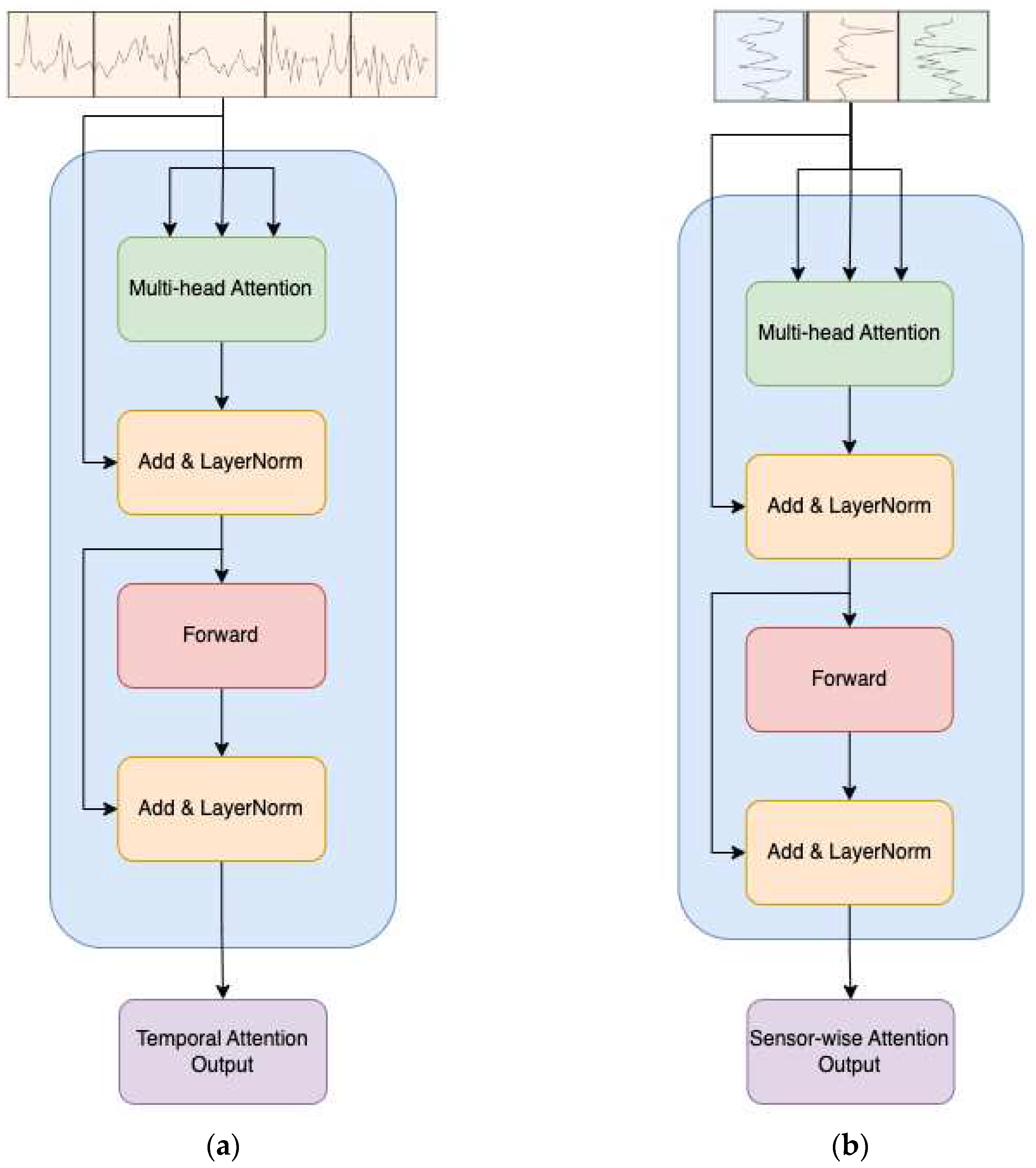
The input is initially partitioned into D distinct fragments. Each fragment X : ,    d , : ( e ) is then fed into the temporal attention calculation block, closely resembling the conventional multi-head self-attention (MSA) [33], as depicted in Figure 3 (a). This block is responsible for capturing temporal dependencies within each sensor's readings.
MSA is a critical mechanism in the Transformer architecture, particularly beneficial for tasks involving sequential data processing. In the original Transformer formulation, the self-attention mechanism is enhanced by introducing multiple attention heads. This extension allows the model to attend to different positions in the input sequence simultaneously and learn diverse relationships between elements.
The standard self-attention mechanism computes attention scores using the following equation for a single attention head:
A t t e n t i o n Q , K , V = s o f t m a x Q K T d k V
Here, Q , K , and V denote the query, key, and value matrices, respectively. The softmax operation normalizes the attention scores, and d k is a scaling factor to control the magnitude of the scores. The resulting attention values are then multiplied by the value matrix to obtain the weighted sum.
In the multi-head attention mechanism, the process is parallelized across h attention heads, each with distinct learned linear projections of the input Q , K , and V matrices. The final output is obtained by concatenating the outputs from all attention heads with a linear transformation:
M S A Q , K , V = C o n c a t h e a d 1 , h e a d 2 , , h e a d h W o
Here, W o is a learned linear transformation matrix applied to the concatenated outputs. Then, the temporal attention block can be expressed as follows:
X ^ : , d , : e = L a y e r N o r m ( X : , d , : e + M S A ( X : , d , : e , X : , d , : e , X : , d , : e ) )
X : , d , : t e m p = L a y e r N o r m ( X ^ : , d , : e + F o r w a r d ( X ^ : , d , : e ) )
Following the temporal attention block, X t e m p R K × D × d m o d e l is subsequently fed into the sensor-wise attention block, depicted in Figure 3 (b), to capture sensor-wise attention. The computation within the sensor-wise attention block is analogous to that of the temporal attention block, utilizing the input X k , : , : t e m p . This mechanism allows the model to attend to important sensors and capture relevant features in the context of the temporal sequence.

2.3. Patch Merging

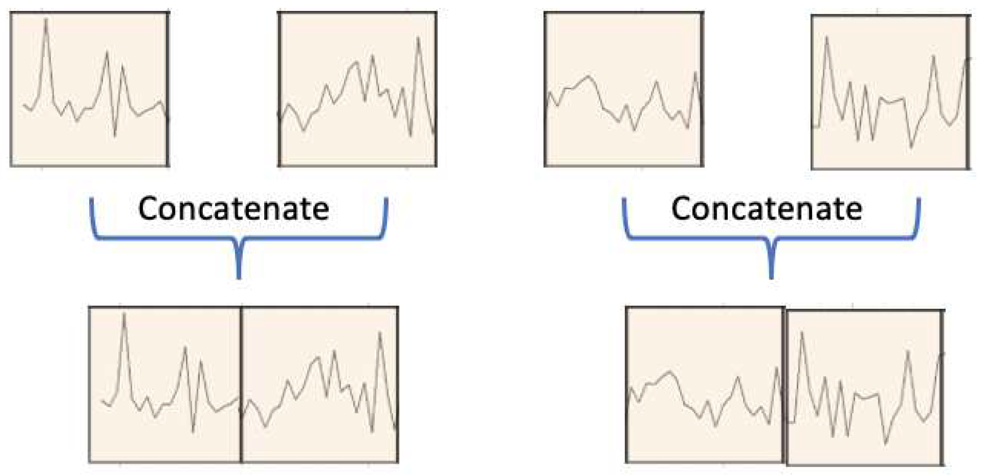
As illustrated in Figure 1, the output of the two-stage attention-based encoder, denoted as X e n c , s , undergoes processing in the patch merging block to generate coarser patches, facilitating multiscale predictions. Specifically, in the patch merging block (see Figure 4), adjacent patches for each sensor are combined in the time domain, creating a coarser patch segmentation. These resultant coarser patches serve as input for the subsequent layer/scale ( s + 1 ) in the encoder. This hierarchical structure enables the model to capture temporal information across different time scales, enhancing its predictive capabilities.
The concatenated coarser patch undergoes an affine transformation to maintain the dimensionality at d m o d e l . The procedure is summarized by the equation below:
X i e n c , s + 1 = B [ X 2 i , d e n c , s ,   X 2 i + 1 , d e n c , s ]
Here, B R d m o d e l × 2 d m o d e l represents a learnable matrix employed for dimensionality preservation during the patch merging process.

2.4. Two-Stage Attention Based Decoder

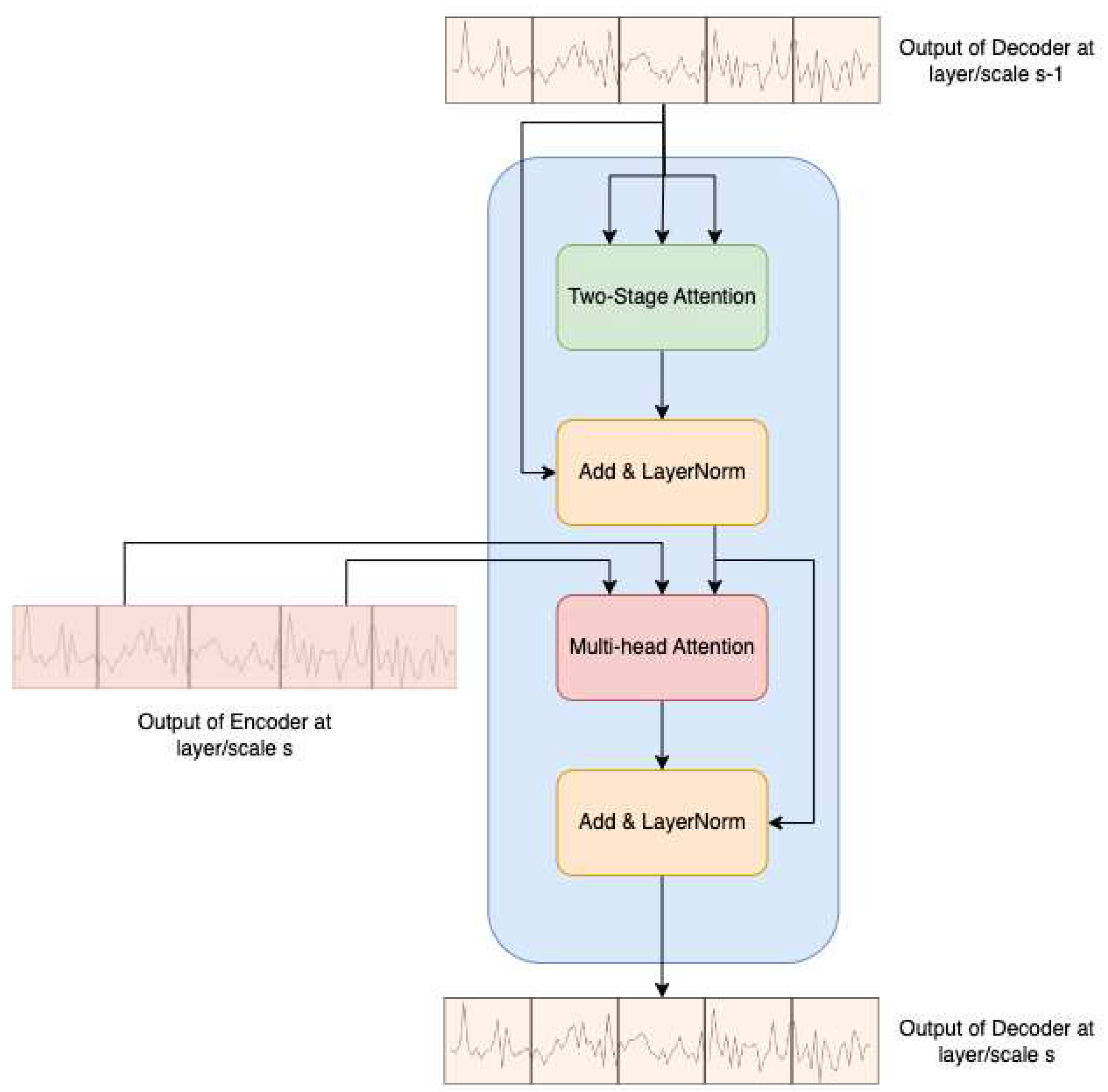
At layer/scale s , the inputs of two-stage attention-based decoder are X e n c , s and X d e c , s 1 , where X d e c , s 1 is the output of the decoder from previous layer/scale s 1 . The decoder architecture closely resembles that of the original Transformer network, with the modification of replacing the masked multi-head self-attention (MMSA) with a two-stage attention mechanism, as illustrated in Figure 5.
In the decoder process, the output of the decoder at the previous layer s 1 undergoes the two-stage attention block, followed by a residual connection and layer normalization. Subsequently, the output of the encoder in the current layer s serves as the keys and values for the MSA block. This modification enhances the decoder's ability to capture both temporal and sensor-wise attention, contributing to improved RUL prediction accuracy. It's important to note that the input of the decoder at the initial layer/scale comprises a fixed positional encoder defined by trigonometric functions, as introduced by Vaswani et al. [33].

2.5. Prediction Layer

As depicted in the right part of Figure 1, the outputs of the decoders at different layers/scales are fed into separate MLPs to further embed the information, enhancing the model's ability to capture intricate patterns for RUL prediction. The outputs from these individual MLP blocks are then concatenated and passed into another MLP to make the final prediction. This hierarchical embedding and fusion process enable the model to capture both local and global dependencies, contributing to improved accuracy in predicting the RUL of turbofan engines.

3. Experimental Results and Analysis

The experiments were performed on a computational system comprising an Intel Core i9 3.6 GHz processor, 64 GB of RAM, and 4 NVIDIA RTX 3080 GPU.
In the following subsections, we will initially present the CMAPSS dataset utilized in our experiments and discuss data preprocessing in Section 3.1. Subsequently, Section 3.2 will delve into the details of hyperparameter tuning and implementation specifics. The performance metrics employed to evaluate the proposed STAR framework are introduced in Section 3.3. The performance results of the STAR framework will be presented and compared with several existing benchmarks in Section 3.4. Finally, in Section 3.5, a set of ablation studies is conducted to demonstrate the importance of each component in our STAR framework.

3.1. Data and Preprocessing

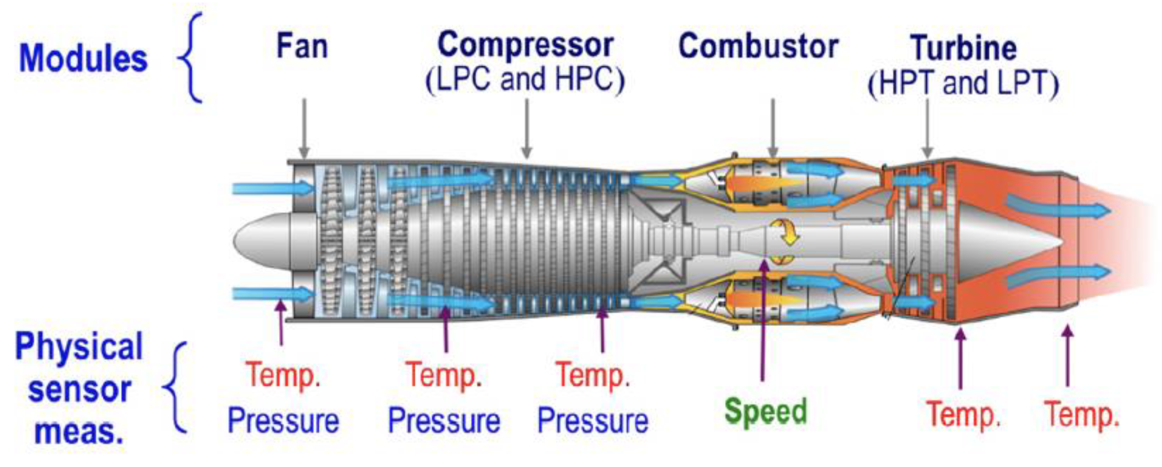
We opted to utilize the NASA Commercial Modular Aero-Propulsion System Simulation (CMAPSS) dataset as the benchmark for assessing our model. Developed by NASA, CMAPSS is an extensive simulation framework designed to replicate the behavior of commercial aircraft turbofan engines, facilitating detailed investigations into engine performance, diagnostics, and prognostics. Widely recognized in the field of Prognostics and Health Management (PHM) for aircraft turbofan engines, the CMAPSS dataset is generated within this simulation environment, providing a valuable repository of multivariate time-series data. Simulating the operation of a fleet of engines under diverse conditions and fault scenarios, the dataset includes sensor readings from various engine components. Researchers leverage this resource to explore and devise methods for tasks such as RUL prediction, fault diagnosis, and performance analysis. Figure 6 illustrates the structure of a turbofan engine within CMAPSS, comprising five modules: fan, low-pressure turbine (LPT), high-pressure turbine (HPT), low-pressure compressor (LPC), and high-pressure compressor (HPC).
The dataset is organized into four sub-datasets, FD001, FD002, FD003, and FD004, based on fault modes and operating conditions, and each sub-dataset is further divided into training and testing subsets as shown in Table 1 below. The training set spans the entire operational lifecycle of the turbofan engine, capturing data from its initial operation to degradation and failure. Conversely, the test set begins at a healthy state and undergoes arbitrary truncation, with the operating time periods leading up to system failure calculated from these truncated data. Additionally, the test set includes the actual RUL values of the test engine, facilitating the assessment of the model’s accuracy in predicting the time remaining until failure.
Each observation in the dataset is a snapshot of data taken during a single operating time cycle with 21 onboard sensors monitoring the engine's health status, as detailed in Table 2.
However, not all sensors contribute useful information for RUL prediction, as some remain constant until failure [34,38,45]. Following the approach outlined in [34], we selectively incorporate data from 14 sensors (sensors 2, 3, 4, 7, 8, 9, 11, 12, 13, 14, 15, 17, 20, 21) into our training and testing processes. Additionally, we apply max-min normalization to the sensor readings, which is expressed by the formula:
x = x x m i n   x m a x x m i n
Here, x represents the original sensor readings, x m i n   is the minimum value of the sensor readings, and x m a x   is the maximum value of the sensor readings. This normalization technique scales the sensor values to a consistent range [0, 1], promoting uniformity and aiding in the training process for effective RUL prediction models. The selective inclusion of sensors and normalization contribute to improved model performance and robustness [49].
In traditional RUL estimation, the common practice involves assigning target values that decrease linearly with time, assuming a linear degradation of the system's health over its operational life. However, this simplified assumption may not accurately reflect the real-world behavior of system degradation, especially during the initial stages when degradation is typically negligible. To address this limitation, our approach, inspired by a piece-wise linear RUL target function proposed in previous studies [49,50], introduces a more nuanced labeling strategy for RUL in the CMAPSS datasets. In our approach, RULs are initially labeled with a constant value ( R U L m a x ), representing a phase of minimal degradation. Subsequently, the system enters a phase of linear degradation until it reaches failure. This truncated linear model better captures the complex evolution of RUL, considering varying degradation rates over different life cycle phases. By aligning our RUL labeling with the actual behavior of turbofan engines, our method provides a more realistic representation of system health progression, especially during the initial stages of operation.

3.2. Hyperparameter Tuning

The hyperparameter tuning process for the proposed STAR model involves an extensive grid search to identify the optimal configuration in terms of root mean squared error (RMSE). The grid search encompasses key hyperparameters, such as learning rate, batch size, optimizer, input time series length, the number of layers/scales for multiscale prediction, and the dimension of embedding space and number of heads in MSA. A detailed breakdown of the possible range and grid for these hyperparameters is provided in Table 3. This grid search methodology allows for a comprehensive examination of various parameter combinations, facilitating the identification of the most effective setup for RUL prediction.
The optimal hyperparameter combinations for FD001 to FD004 are presented in Table 4. Subsequently, the prediction model is instantiated using these sets of hyperparameters to predict RUL for testing engines.
It is evident from the results that FD002 and FD004 datasets necessitate a longer time series length, a greater number of layers/scales, and more heads in MSA compared to FD001 and FD003 datasets. We posit that this disparity arises from the fact that FD002 and FD004 datasets are simulated under diverse operational conditions. Consequently, they demand a more intricate network structure to extract valuable features for RUL prediction. Additionally, these datasets require longer input sequences, containing more information to generate accurate predictions.

3.3. Evaluation Metric

In evaluating the predictive performance of the proposed model for RUL, two key metrics are employed: the RMSE and an effectiveness Score. The RMSE, expressed by Equation (7), is a widely used metric in RUL estimation evaluation, providing equal penalty weights for both underestimation and overestimation of RUL. It calculates the square root of the mean squared differences between the true RULs values y i and the predicted RUL values y ^ i .
R M S E = i = 1 n y i y ^ i 2 N
On the other hand, the effectiveness Score, defined by Equation (8), introduces distinct penalty weights for the direction of prediction deviation. The Score penalizes advancements (where y ^ i is smaller than y i ) with a smaller coefficient, recognizing the opportunity for proactive maintenance planning. Conversely, when predictions lag (where y ^ i is larger than y i ), a larger penalty coefficient is applied, reflecting the potential for more severe consequences when the maintenance is performed too late.
S c o r e = i = 1 N e y i y ^ i 13 1 ,     d < 0 i = 1 N e y i y ^ i 10 1 ,     d 0

3.4. RUL Prediction

In this section, we rigorously evaluate the performance of the proposed STAR framework for RUL prediction. To benchmark its effectiveness, we compare the proposed model against a suite of existing methods widely recognized in the field. These methods include MLP [51], support vector regression (SVR) [51], CNN [51], LSTM [49], BiLSTM [52], DAG [53], the gated convolutional Transformer (GCT) [34], CNN + LSTM [54], multi-head CNN + LSTM [55], B-LSTM [31], BiLSTM attention model [56], DAST [44], DLformer [35], and BiLSTM-DAE-Transformer [40]. Table 5 shows the comparison results.
As presented in Table 5, the proposed STAR framework consistently outperforms existing RUL prediction models across all datasets, showcasing its superior predictive capabilities. Notably, for FD001 and FD002 datasets, our method demonstrates the best performance, achieving the lowest RMSE and Score values. Remarkably, the STAR framework exhibits significant improvements in both RMSE and Score metrics for the challenging FD002 dataset, surpassing state-of-the-art models by 12% and 15% in terms of RMSE and Score, respectively. This highlights the effectiveness of capturing sensor-wise attention, which is particularly crucial in cases such as FD002, simulated under diverse operating conditions. For the FD003 dataset, our STAR framework attains the best performance in terms of RMSE and the second-best performance in terms of Score. This observation suggests a tendency to underestimate RUL for this dataset, leading to a larger penalty when calculating the Score metric. Consequently, while our model excels when evaluated based on RMSE, there is a slight deviation when employing the Score metric. Contrarily, for the FD004 dataset, the trends are reversed compared to FD003. In this scenario, our model achieves the second-best performance in terms of RMSE while securing the top position in Score. It is noteworthy that the difference in RMSE between our method and the best model for FD004 (DLformer) is only 0.01, highlighting the competitive performance of the STAR framework.
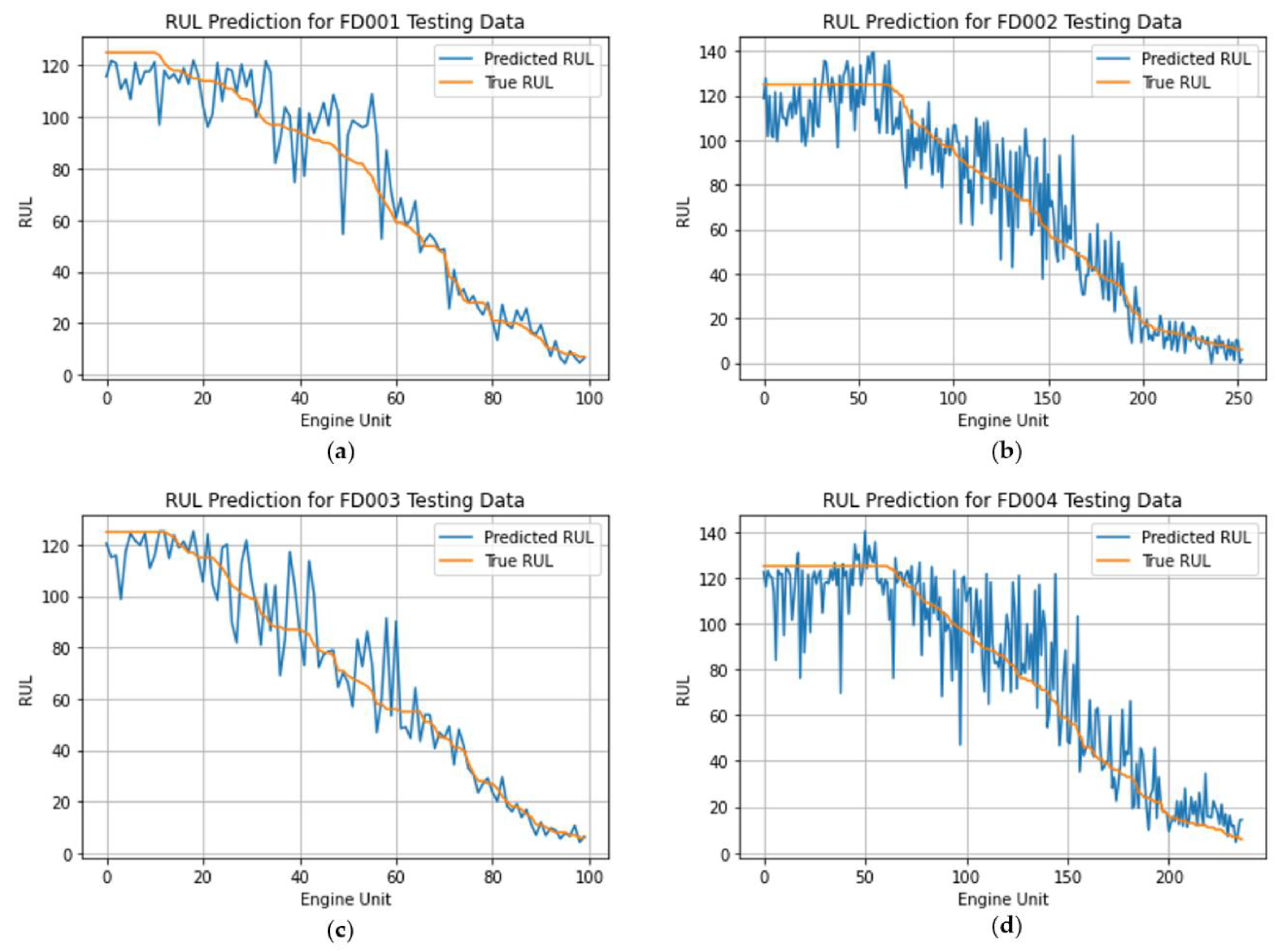
Figure 7 serves as a comprehensive visual representation, offering a detailed comparison between the predicted RUL generated by our STAR model and the ground-truth RULs across the FD001 to FD004 testing datasets. The x-axis corresponds to the Engine Unit Index, while the y-axis depicts the RUL. The graphical depiction provides insights into the model's performance under varying conditions.
For enhanced clarity in visualization, we adhere to the conventional practice of arranging all test sequences along the x-axis in ascending order based on their ground truth RUL. In Figures 7 (a) and (c), the model exhibits notable precision, especially for scenarios where the ground-truth RUL is relatively small (below 60). However, for FD002 and FD004 datasets, the prediction results display a discernible level of noise compared to the smoother outcomes observed in FD001 and FD003. This observed variability may be attributed to differences in operational complexities, as evidenced by varying numbers of operating conditions and fault modes, along with the size of the training dataset. Notably, FD002 and FD004 involve simulations under six distinct operating conditions, while FD001 and FD003 are conducted under a single operating condition. The heightened complexity in FD002 and FD004 likely contributes to the observed noise in predictions, underscoring the model's sensitivity to the intricacies of working conditions and the dataset size across diverse scenarios.

3.5. Ablation Study

In this section, we conduct ablation experiments to assess the impact of individual components in our proposed model. Specifically, we compare the prediction performances, evaluated in terms of RMSE, for the following models, all utilizing the same set of hyperparameters selected from Table 4:
  • STAR: The proposed model with a two-stage attention mechanism and hierarchical encoder-decoder.
  • STAR-Temporal: The proposed model with temporal attention only and a hierarchical encoder-decoder.
  • STAR-SingleScale: The proposed model with a two-stage attention mechanism and hierarchical encoder-decoder, excluding the patch merging step between different layers/scales as depicted in Figure 1.
The findings revealed in Table 6 emphasize the importance of each component in our proposed STAR model, shedding light on their respective contributions to achieving noteworthy prediction performance. Notably, the STAR model without sensor-wise variable attention and multiscale information exhibits a decline in prediction performance, particularly evident in the case of more complex FD002 and FD004 datasets.

4. Conclusions

This paper presents an innovative STAR framework designed for predicting the RUL of turbofan engines. Leveraging a two-stage attention mechanism, our proposed model adeptly captures both temporal and sensor-wise variable attention. By utilizing a hierarchical encoder-decoder structure to integrate multiscale information, the model produces hierarchical predictions, demonstrating superior performance in predicting RUL. Using the CMAPSS dataset, we illustrate the importance of incorporating both temporal attention and sensor-wise variable attention for RUL prediction through a series of numerical experiments. The results highlight the promising potential of the STAR framework in achieving accurate and reliable RUL predictions, thereby contributing to advancements in prognostics for the health management of aircraft engines.
Despite the superior performance demonstrated by the proposed methods in predicting RUL, it’s important to note that the model inherently lacks the ability to provide explanations for its identification of equipment approaching failure. Therefore, a promised area for future research involves incorporating Explainable Artificial Intelligence (XAI) methods, such as SHAP and LIME, to unravel the prediction logic of the model. This enhancement has the potential to increase the applicability of the prediction model in practical scenarios, particularly within the context of CBPM.

Author Contributions

Conceptualization, Z.F. and K.C.; writing, manuscript preparation, Z.F. and W.L.; review and editing, W.L. and K.C.; supervision and project management, K.C.. All authors have read and agreed to the published version of the manuscript.

Funding

This research received no external funding.

Data Availability Statement

The data of this paper came from the NASA Prognostics Center of Excellence, and the data acquisition website was: https://ti.arc.nasa.gov/tech/dash/groups/pcoe/ prognostic-data-repository/#turbofan, accessed on 15 April 2023.

Acknowledgments

Not applicable.

Conflicts of Interest

The authors declare no conflicts of interest.

References

  1. Peng, Y.; Dong, M.; Zuo, M.J. Current Status of Machine Prognostics in Condition-Based Maintenance: A Review. Int. J. Adv. Manuf. Technol. 2010, 50, 297–313. [Google Scholar] [CrossRef]
  2. Fan, Z.; Chang, K.; Ji, R.; Chen, G. Data Fusion for Optimal Condition-Based Aircraft Fleet Maintenance with Predictive Analytics. J. Adv. Inf. Fusion 2023, In Press.
  3. Si, X.-S.; Wang, W.; Hu, C.-H.; Zhou, D.-H.; Pecht, M.G. Remaining Useful Life Estimation Based on a Nonlinear Diffusion Degradation Process. IEEE Trans. Reliab. 2012, 61, 50–67. [Google Scholar] [CrossRef]
  4. Bolander, N.; Qiu, H.; Eklund, N.; Hindle, E.; Rosenfeld, T. Physics-Based Remaining Useful Life Prediction for Aircraft Engine Bearing Prognosis. Annu. Conf. PHM Soc. 2009, 1. [Google Scholar]
  5. Roemer, M.J.; Kacprzynski, G.J. Advanced Diagnostics and Prognostics for Gas Turbine Engine Risk Assessment. In Proceedings of the 2000 IEEE Aerospace Conference. Proceedings (Cat. No.00TH8484); March 2000; Vol. 6; pp. 345–353. [Google Scholar]
  6. Luo, J.; Namburu, M.; Pattipati, K.; Qiao, L.; Kawamoto, M.; Chigusa, S. Model-Based Prognostic Techniques [Maintenance Applications]. In Proceedings of the Proceedings AUTOTESTCON 2003. IEEE Systems Readiness Technology Conference.; September 2003; pp. 330–340. [Google Scholar]
  7. Ray, A.; Tangirala, S. Stochastic Modeling of Fatigue Crack Dynamics for On-Line Failure Prognostics. IEEE Trans. Control Syst. Technol. 1996, 4, 443–451. [Google Scholar] [CrossRef]
  8. Li, Y.; Billington, S.; Zhang, C.; Kurfess, T.; Danyluk, S.; Liang, S. Adaptive Prognostics for Rolling Element Bearing Condition. Mech. Syst. Signal Process. 1999, 13, 103–113. [Google Scholar] [CrossRef]
  9. Kacprzynski, G.J.; Sarlashkar, A.; Roemer, M.J.; Hess, A.; Hardman, B. Predicting Remaining Life by Fusing the Physics of Failure Modeling with Diagnostics. JOM 2004, 56, 29–35. [Google Scholar] [CrossRef]
  10. Oppenheimer, C.H.; Loparo, K.A. Physically Based Diagnosis and Prognosis of Cracked Rotor Shafts. In Proceedings of the Component and Systems Diagnostics, Prognostics, and Health Management II; SPIE, July 16 2002; Vol. 4733; pp. 122–132. [Google Scholar]
  11. Giantomassi, A.; Ferracuti, F.; Benini, A.; Ippoliti, G.; Longhi, S.; Petrucci, A. Hidden Markov Model for Health Estimation and Prognosis of Turbofan Engines.; American Society of Mechanical Engineers Digital Collection, June 12 2012; pp. 681–689.
  12. Lin, J.; Liao, G.; Chen, M.; Yin, H. Two-Phase Degradation Modeling and Remaining Useful Life Prediction Using Nonlinear Wiener Process. Comput. Ind. Eng. 2021, 160, 107533. [Google Scholar] [CrossRef]
  13. Yu, W.; Tu, W.; Kim, I.Y.; Mechefske, C. A Nonlinear-Drift-Driven Wiener Process Model for Remaining Useful Life Estimation Considering Three Sources of Variability. Reliab. Eng. Syst. Saf. 2021, 212, 107631. [Google Scholar] [CrossRef]
  14. Feng, D.; Xiao, M.; Liu, Y.; Song, H.; Yang, Z.; Zhang, L. A Kernel Principal Component Analysis–Based Degradation Model and Remaining Useful Life Estimation for the Turbofan Engine. Adv. Mech. Eng. 2016, 8, 1687814016650169. [Google Scholar] [CrossRef]
  15. Lv, Y.; Zheng, P.; Yuan, J.; Cao, X. A Predictive Maintenance Strategy for Multi-Component Systems Based on Components’ Remaining Useful Life Prediction. Mathematics 2023, 11, 3884. [Google Scholar] [CrossRef]
  16. Zhang, Y.; Guo, G.; Yang, F.; Zheng, Y.; Zhai, F. Prediction of Tool Remaining Useful Life Based on NHPP-WPHM. Mathematics 2023, 11, 1837. [Google Scholar] [CrossRef]
  17. Greitzer, F.L.; Li, W.; Laskey, K.B.; Lee, J.; Purl, J. Experimental Investigation of Technical and Human Factors Related to Phishing Susceptibility. ACM Trans. Soc. Comput. 2021, 4, 8:1–8:48. [Google Scholar] [CrossRef]
  18. Li, W.; Lee, J.; Purl, J.; Greitzer, F.; Yousefi, B.; Laskey, K. Experimental Investigation of Demographic Factors Related to Phishing Susceptibility; 2020; ISBN 978-0-9981331-3-3.
  19. Li, W.; Finsa, M.M.; Laskey, K.B.; Houser, P.; Douglas-Bate, R. Groundwater Level Prediction with Machine Learning to Support Sustainable Irrigation in Water Scarcity Regions. Water 2023, 15, 3473. [Google Scholar] [CrossRef]
  20. Liu, W.; Zou, P.; Jiang, D.; Quan, X.; Dai, H. Computing River Discharge Using Water Surface Elevation Based on Deep Learning Networks. Water 2023, 15, 3759. [Google Scholar] [CrossRef]
  21. Fan, Z.; Chang, K.; Raz, A.K.; Harvey, A.; Chen, G. Sensor Tasking for Space Situation Awareness: Combining Reinforcement Learning and Causality. In Proceedings of the 2023 IEEE Aerospace Conference; March 2023; pp. 1–9. [Google Scholar]
  22. Zhou, W. Condition State-Based Decision Making in Evolving Systems: Applications in Asset Management and Delivery. Ph.D., George Mason University: United States -- Virginia, 2023.
  23. Peng, C.; Chen, Y.; Chen, Q.; Tang, Z.; Li, L.; Gui, W. A Remaining Useful Life Prognosis of Turbofan Engine Using Temporal and Spatial Feature Fusion. Sensors 2021, 21, 418. [Google Scholar] [CrossRef] [PubMed]
  24. Remadna, I.; Terrissa, S.L.; Zemouri, R.; Ayad, S.; Zerhouni, N. Leveraging the Power of the Combination of CNN and Bi-Directional LSTM Networks for Aircraft Engine RUL Estimation. In Proceedings of the 2020 Prognostics and Health Management Conference (PHM-Besançon); May 2020; pp. 116–121. [Google Scholar]
  25. Hong, C.W.; Lee, C.; Lee, K.; Ko, M.-S.; Kim, D.E.; Hur, K. Remaining Useful Life Prognosis for Turbofan Engine Using Explainable Deep Neural Networks with Dimensionality Reduction. Sensors 2020, 20, 6626. [Google Scholar] [CrossRef] [PubMed]
  26. Lundberg, S.M.; Lee, S.-I. A Unified Approach to Interpreting Model Predictions. In Proceedings of the Advances in Neural Information Processing Systems; Curran Associates, Inc., 2017; Vol. 30. [Google Scholar]
  27. Rosa, T.G. da; Melani, A.H. de A.; Pereira, F.H.; Kashiwagi, F.N.; Souza, G.F.M. de; Salles, G.M.D.O. Semi-Supervised Framework with Autoencoder-Based Neural Networks for Fault Prognosis. Sensors 2022, 22, 9738. [Google Scholar] [CrossRef] [PubMed]
  28. Ji, S.; Han, X.; Hou, Y.; Song, Y.; Du, Q. Remaining Useful Life Prediction of Airplane Engine Based on PCA–BLSTM. Sensors 2020, 20, 4537. [Google Scholar] [CrossRef] [PubMed]
  29. Peng, C.; Wu, J.; Wang, Q.; Gui, W.; Tang, Z. Remaining Useful Life Prediction Using Dual-Channel LSTM with Time Feature and Its Difference. Entropy 2022, 24, 1818. [Google Scholar] [CrossRef]
  30. Zhao, C.; Huang, X.; Li, Y.; Yousaf Iqbal, M. A Double-Channel Hybrid Deep Neural Network Based on CNN and BiLSTM for Remaining Useful Life Prediction. Sensors 2020, 20, 7109. [Google Scholar] [CrossRef]
  31. Wang, X.; Huang, T.; Zhu, K.; Zhao, X. LSTM-Based Broad Learning System for Remaining Useful Life Prediction. Mathematics 2022, 10, 2066. [Google Scholar] [CrossRef]
  32. Yu, W.; Kim, I.Y.; Mechefske, C. Remaining Useful Life Estimation Using a Bidirectional Recurrent Neural Network Based Autoencoder Scheme. Mech. Syst. Signal Process. 2019, 129, 764–780. [Google Scholar] [CrossRef]
  33. Vaswani, A.; Shazeer, N.; Parmar, N.; Uszkoreit, J.; Jones, L.; Gomez, A.N.; Kaiser, Ł.; Polosukhin, I. Attention Is All You Need. In Proceedings of the Advances in Neural Information Processing Systems; Curran Associates, Inc., 2017; Vol. 30. [Google Scholar]
  34. Mo, Y.; Wu, Q.; Li, X.; Huang, B. Remaining Useful Life Estimation via Transformer Encoder Enhanced by a Gated Convolutional Unit. J. Intell. Manuf. 2021, 32, 1997–2006. [Google Scholar] [CrossRef]
  35. Ren, L.; Wang, H.; Huang, G. DLformer: A Dynamic Length Transformer-Based Network for Efficient Feature Representation in Remaining Useful Life Prediction. IEEE Trans. Neural Netw. Learn. Syst. 2023, 1–11. [Google Scholar] [CrossRef] [PubMed]
  36. Zhang, Y.; Su, C.; Wu, J.; Liu, H.; Xie, M. Trend-Augmented and Temporal-Featured Transformer Network with Multi-Sensor Signals for Remaining Useful Life Prediction. Reliab. Eng. Syst. Saf. 2024, 241, 109662. [Google Scholar] [CrossRef]
  37. Li, Y.; Chen, Y.; Shao, H.; Zhang, H. A Novel Dual Attention Mechanism Combined with Knowledge for Remaining Useful Life Prediction Based on Gated Recurrent Units. Reliab. Eng. Syst. Saf. 2023, 239, 109514. [Google Scholar] [CrossRef]
  38. Peng, H.; Jiang, B.; Mao, Z.; Liu, S. Local Enhancing Transformer With Temporal Convolutional Attention Mechanism for Bearings Remaining Useful Life Prediction. IEEE Trans. Instrum. Meas. 2023, 72, 1–12. [Google Scholar] [CrossRef]
  39. Xiang, F.; Zhang, Y.; Zhang, S.; Wang, Z.; Qiu, L.; Choi, J.-H. Bayesian Gated-Transformer Model for Risk-Aware Prediction of Aero-Engine Remaining Useful Life. Expert Syst. Appl. 2024, 238, 121859. [Google Scholar] [CrossRef]
  40. Fan, Z.; Li, W.; Chang, K.-C. A Bidirectional Long Short-Term Memory Autoencoder Transformer for Remaining Useful Life Estimation. Mathematics 2023, 11, 4972. [Google Scholar] [CrossRef]
  41. Xue, W.; Zhou, T.; Wen, Q.; Gao, J.; Ding, B.; Jin, R. Make Transformer Great Again for Time Series Forecasting: Channel Aligned Robust Dual Transformer 2023.
  42. Nie, Y.; Nguyen, N.H.; Sinthong, P.; Kalagnanam, J. A Time Series Is Worth 64 Words: Long-Term Forecasting with Transformers 2023.
  43. Zhang, Y.; Yan, J. Crossformer: Transformer Utilizing Cross-Dimension Dependency for Multivariate Time Series Forecasting.; September 29 2022.
  44. Zhang, Z.; Song, W.; Li, Q. Dual-Aspect Self-Attention Based on Transformer for Remaining Useful Life Prediction. IEEE Trans. Instrum. Meas. 2022, 71, 1–11. [Google Scholar] [CrossRef]
  45. Chadha, G.S.; Shah, S.R.B.; Schwung, A.; Ding, S.X. Shared Temporal Attention Transformer for Remaining Useful Lifetime Estimation. 2022, 10.
  46. Liu, Z.; Lin, Y.; Cao, Y.; Hu, H.; Wei, Y.; Zhang, Z.; Lin, S.; Guo, B. Swin Transformer: Hierarchical Vision Transformer Using Shifted Windows.; 2021; pp. 10012–10022.
  47. Devlin, J.; Chang, M.-W.; Lee, K.; Toutanova, K. BERT: Pre-Training of Deep Bidirectional Transformers for Language Understanding 2019.
  48. Saxena, A.; Goebel, K.; Simon, D.; Eklund, N. Damage Propagation Modeling for Aircraft Engine Run-to-Failure Simulation. In Proceedings of the 2008 International Conference on Prognostics and Health Management; October 2008; pp. 1–9. [Google Scholar]
  49. Zheng, S.; Ristovski, K.; Farahat, A.; Gupta, C. Long Short-Term Memory Network for Remaining Useful Life Estimation. In Proceedings of the 2017 IEEE International Conference on Prognostics and Health Management (ICPHM); June 2017; pp. 88–95. [Google Scholar]
  50. Wu, Q.; Ding, K.; Huang, B. Approach for Fault Prognosis Using Recurrent Neural Network. J. Intell. Manuf. 2020, 31, 1621–1633. [Google Scholar] [CrossRef]
  51. Sateesh Babu, G.; Zhao, P.; Li, X.-L. Deep Convolutional Neural Network Based Regression Approach for Estimation of Remaining Useful Life. In Proceedings of the Database Systems for Advanced Applications; Navathe, S.B., Wu, W., Shekhar, S., Du, X., Wang, X.S., Xiong, H., Eds.; Springer International Publishing: Cham, 2016; pp. 214–228. [Google Scholar]
  52. Wang, J.; Wen, G.; Yang, S.; Liu, Y. Remaining Useful Life Estimation in Prognostics Using Deep Bidirectional LSTM Neural Network. In Proceedings of the 2018 Prognostics and System Health Management Conference (PHM-Chongqing); October 2018; pp. 1037–1042. [Google Scholar]
  53. Li, J.; Li, X.; He, D. A Directed Acyclic Graph Network Combined With CNN and LSTM for Remaining Useful Life Prediction. IEEE Access 2019, 7, 75464–75475. [Google Scholar] [CrossRef]
  54. Kong, Z.; Cui, Y.; Xia, Z.; Lv, H. Convolution and Long Short-Term Memory Hybrid Deep Neural Networks for Remaining Useful Life Prognostics. Appl. Sci. 2019, 9, 4156. [Google Scholar] [CrossRef]
  55. Mo, H.; Lucca, F.; Malacarne, J.; Iacca, G. Multi-Head CNN-LSTM with Prediction Error Analysis for Remaining Useful Life Prediction. In Proceedings of the 2020 27th Conference of Open Innovations Association (FRUCT); September 2020; pp. 164–171. [Google Scholar]
  56. Liu, Y.; Zhang, X.; Guo, W.; Bian, H.; He, Y.; Liu, Z. Prediction of Remaining Useful Life of Turbofan Engine Based on Optimized Model. In Proceedings of the 2021 IEEE 20th International Conference on Trust, Security and Privacy in Computing and Communications (TrustCom); October 2021; pp. 1473–1477. [Google Scholar]
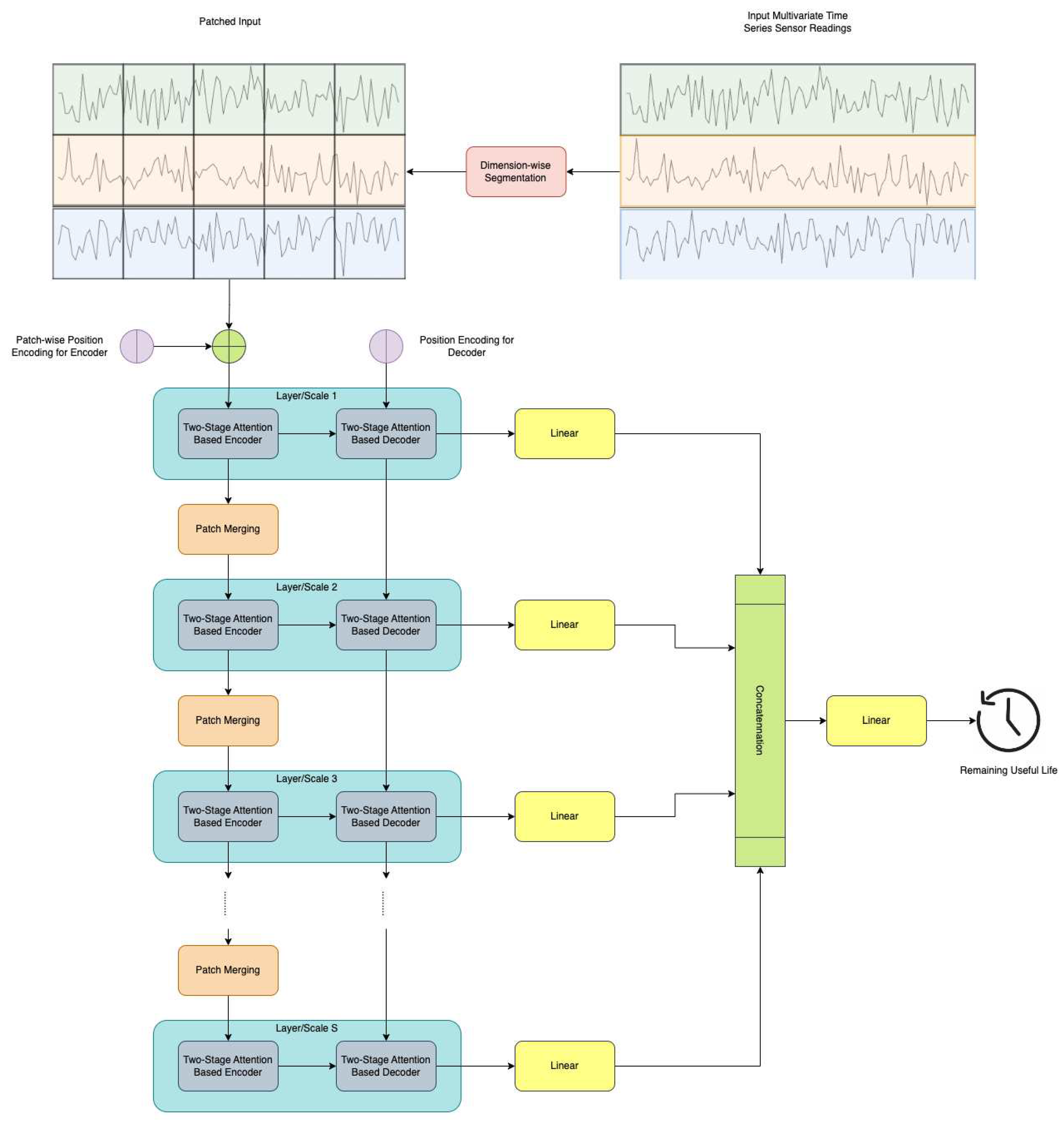
Figure 1. Overall structure of the proposed STAR frameworks.
Preprints 94833 g001
Figure 2. Two-stage attention-based encoder.
Preprints 94833 g002
Figure 3. Temporal and sensor-wise variable attentions. (a) Network architecture for temporal attention. (b) Network architecture for sensor-wise variable attention.
Preprints 94833 g003
Figure 4. Two-stage attention-based encoder.
Preprints 94833 g004
Figure 5. Two-stage attention-based decoder.
Preprints 94833 g005
Figure 6. Turbofan engine model [48].
Preprints 94833 g006
Figure 7. Comparisons between predicted RUL and ground truth RUL for all four CMAPSS datasets. The x-axis in the figures corresponds to the Engine Unit Index, while the y-axis represents the Remaining Useful Life. (a) RUL prediction for FD001; (b) RUL prediction for FD002; (c) RUL prediction for FD003; (d) RUL prediction for FD004.
Preprints 94833 g007
Table 1. Parameters of the C-MAPSS dataset.
Dataset FD001 FD002 FD003 FD004
No. of Training Engines 100 260 100 249
No. of Testing Engines 100 259 100 248
No. of Operating Conditions 1 6 1 6
No. of Fault Modes 1 1 2 2
Table 2. C-MAPSS Monitoring Sensor Data Description.
Symbol Description Units
T2 Total temperature at fan inlet R
T24 Total temperature at LPC inlet R
T30 Total temperature at HPC inlet R
T50 Total temperature at LPT inlet R
P2 Pressure at fan inlet psia
P15 Total pressure in bypass-duct psia
P30 Total pressure at HPC outlet psia
Nf Physical fan speed rpm
Ne Physical core speed rpm
epr Engine pressure ratio -
Ps30 Static pressure at HPC outlet psia
Phi Ratio of fuel flow to Ps30 pps/psi
NRf Corrected fan speed rpm
NRe Corrected core speed rpm
BPR Bypass ratio -
farB Burner fuel-air ratio -
htBleed Bleed Enthalpy -
Bf-dmd Demanded fan speed rpm
PCNfR-dmd Demanded corrected fan speed rpm
W31 HPT coolant bleed lbm/s
W32 LPT coolant bleed lbm/s
Table 3. Hyperparameters and Ranges.
Hyperparameter Range
Learning Rate [0.0001,0.01]
Batch Size 16, 32, 64
Optimizer Adam, SGD, RMSProp
Time Series Length 32, 48, 64
Number of Layers/Scales 1, 2, 3, 4
Dimension of Embedding Space 128, 256, 512, 1024
Number of Head for MSA 1, 2, 4, 6
Table 4. Best hyperparameter combinations for FD001, FD002, FD003 and FD004 data sets.
Hyperparameter FD001 FD002 FD003 FD004
Learning Rate 0.0002 0.0002 0.0002 0.0002
Batch Size 32 64 32 64
Optimizer Adam Adam Adam Adam
Time Series Length 32 64 48 64
Number of Layers/Scales 3 4 1 4
Dimension of Embedding Space 128 64 128 256
Number of Head for MSA 1 4 1 4
Table 5. Performance comparison. The bold number represents the best model, while the underscore number represents the second-best model.
Method FD001 FD002 FD003 FD004
RMSE Score RMSE Score RMSE Score RMSE Score
MLP (2016) 37.56 - 80.03 - 37.39 - 77.37 -
SVR (2016) 20.96 - 42.00 - 21.05 - 45.35 -
CNN (2016) 18.45 - 30.29 - 19.82 - 29.16 -
LSTM (2017) 16.14 338 24.49 4450 16.18 852 28.17 5550
BiLSTM (2018) 13.65 295 23.18 4130 13.74 317 24.86 5430
DAG (2019) 11.96 229 20.34 2730 12.46 535 22.43 3370
CNN + LSTM (2019) 16.16 303 20.44 3440 17.12 1420 23.25 4630
Multi-head CNN + LSTM (2020) 12.19 259 19.93 4350 12.85 343 22.89 4340
GCT (2021) 11.27 - 22.81 - 11.42 - 24.86 -
BiLSTM Attention (2021) 13.78 255 15.94 1280 14.36 438 16.96 1650
B-LSTM (2022) 12.45 279 15.36 4250 13.37 356 16.24 5220
DAST (2022) 11.43 203 15.25 924 11.32 154 18.23 1490
DLformer (2023) - - 15.93 1283 - - 15.86 1601
BiLSTM-DAE-Transformer (2023) 10.98 186 16.12 2937 11.14 252 18.15 3840
Proposed Method 10.61 169 13.47 784 10.71 202 15.87 1449
Table 6. Ablation study of the proposed STAR architecture.
Model FD001 FD002 FD003 FD004
STAR 10.61 13.47 10.71 15.87
STAR-Temporal 11.62 16.67 12.01 18.44
STAR-SingleScale 12.33 16.11 12.49 17.71
Disclaimer/Publisher’s Note: The statements, opinions and data contained in all publications are solely those of the individual author(s) and contributor(s) and not of MDPI and/or the editor(s). MDPI and/or the editor(s) disclaim responsibility for any injury to people or property resulting from any ideas, methods, instructions or products referred to in the content.
Copyright: This open access article is published under a Creative Commons CC BY 4.0 license, which permit the free download, distribution, and reuse, provided that the author and preprint are cited in any reuse.
Prerpints.org logo

Preprints.org is a free preprint server supported by MDPI in Basel, Switzerland.

Subscribe

© 2024 MDPI (Basel, Switzerland) unless otherwise stated