Effect of Network Architecture on Physics-Informed Deep Learning of the Reynolds-Averaged Turbulent Flow Field around Cylinders without Training Data

Preprint

Article

Effect of Network Architecture on Physics-Informed Deep Learning of the Reynolds-Averaged Turbulent Flow Field around Cylinders without Training Data

Altmetrics

Downloads

142

Views

133

Comments

A peer-reviewed article of this preprint also exists.

Jan Hauke Harmening^*,

Franz-Josef Peitzmann,

Ould el Moctar

Jan Hauke Harmening^*,

Franz-Josef Peitzmann,

Ould el Moctar

This version is not peer-reviewed

Submitted:

28 December 2023

Posted:

29 December 2023

You are already at the latest version

Alerts

Abstract

Unsupervised physics-informed deep learning can be used to solve computational physics problems by training neural networks to satisfy the underlying equations and boundary conditions without labeled data. Parameters such as network architecture and training method determine the training success. However, the best choice is unknown a priori as it is case specific. Here, we investigated network shapes, sizes, and types for unsupervised physics-informed deep learning of the two-dimensional Reynolds-averaged flow around cylinders. We trained mixed-variable networks and compared them to traditional models. Several network architectures with different shape factors and sizes were evaluated. The models were trained to solve the Reynolds-averaged Navier-Stokes equations incorporating Prandtl's mixing length turbulence model. No training data were deployed to train the models. The superiority of the mixed-variable approach was confirmed for the investigated high Reynolds number flow. The mixed-variable models were sensitive to the network shape. For the two cylinders, differently deep networks showed superior performance. The best fitting models were able to capture important flow phenomena such as stagnation regions, boundary layers, flow separation, and recirculation. We also encountered difficulties when predicting high Reynolds number flows without training data

Keywords:

Subject: Computer Science and Mathematics - Artificial Intelligence and Machine Learning

1. Introduction

Neural networks (NNs) can be used to approximate arbitrary nonlinear function and its derivatives [1]. However, deep learning (DL) requires large data sets to train these networks [2]. Physics-informed neural networks (PINNs) have attracted a growing interest, as the required amount of training data can be significantly reduced by deploying physics-informed DL. PINNs are NNs that are trained to respect given laws of physics by utilizing a composed loss function that considers residuals of the underlying physics equations and boundary conditions. Physics-informed DL has been demonstrated by Lagaris et al. [3] who used PINNs to solve different differential equations. Later, Raissi et al. [4,5,6] extended this research further and trained several partial differential equations without relying on training data. These studies proved the effectiveness of PINNs and motivated a growing number of investigations in all fields of computational physics.

In the field of fluid dynamics, a variety of research has been carried out. Many investigations focused on laminar flows at low Reynolds numbers [7,8,9,10,11]. Several investigations covered turbulent flows at high Reynolds numbers, and PINNs were trained to solve the Reynolds-averaged Navier-Stokes (RANS) equations. High Reynolds number flows are important research objects for physics-informed DL as most technical flows are subject to high Reynolds numbers and additional turbulence modeling equations, strong convection, as well as high gradients impose challenges to the training success. RANS solutions obtained by PINNs could be applied to surrogate modeling [12] or optimization problems [13] to replace traditional computational fluid dynamics (CFD) calculations of the RANS equations. Several RANS-PINN studies have been conducted for high Reynolds number flows incorporating turbulence models such as Prandtl’s mixing length model [13,14], the k-

ϵ

model [15], the k-

ω

model [14], the Spalart-Allmaras (SA) model [16], as well as equation-free modeling approaches [14,17,18]. This encouraging research, which demonstrated the capabilities of PINNs, incorporated labeled training data into the training routine of the PINN [14,15,16,18], trained parts of the complete flow field using unsupervised DL [17,18], or trained flows without separation without using training data [13]. Hence, the evaluation of unsupervised physics-informed DL methods applied to complete flow fields featuring flow separation at elevated Reynolds numbers remains an open question.

Rao et al. [19] presented a mixed-variable approach of superior accuracy for a low Reynolds number flow around a cylinder without using training data. Motivated by their results, we evaluated the unsupervised mixed-variable method applied to a high Reynolds number flow considering RANS turbulence modeling. To conduct a comparative study, we trained several PINNs to predict the two-dimensional Reynolds-averaged turbulent flow field around two cylinders. We compared the mixed-variable method to traditional PINNs and evaluated various network architectures to identify the most accurate network shape and size. We used the PINNs to solve the RANS equations and applied Prandtl’s mixing length model to model turbulence. The PINN predictions were compared with CFD results as well as experimental measurements. To our knowledge, this is the first detailed report of unsupervised physics-informed DL learning of the RANS equations for a complete flow field featuring flow separation at an elevated Reynolds number. The motivation of this work was to explore and evaluate unsupervised DL methods and network architectures with respect to their prediction accuracy of Reynolds-averaged flows when no training data are provided.

2. Method

2.1. Geometry

We investigated the two-dimensional flow around a circular cylinder as well as a square cylinder. Figure 1 illustrates the cylinder geometries. We considered a fluid with a density

ρ

of 1 kg/m³ and an inlet velocity of 1 m/s. Dimensions and inlet velocity were chosen to yield a scaled problem with network inputs and outputs ranging between -1 and +1 as closely as possible. The resulting flow fields featured important phenomena, such as stagnation points, high gradient boundary layers, flow separation, and wakes. The two geometries exemplified curved and cornered obstacles that impose different flow separation mechanisms triggered at the rounded or cornered walls.

We employed three different versions of the cylinder geometries as presented in Table 1. Geometries G1 and G2 were used to evaluate the effect of network architecture, network shape, and PINN methods for different cylinder shapes at an elevated Reynolds number. The large scale of the cylinders allowed more accurate and spatially detailed PINN predictions. This set up represented a channel flow and allowed comparison to a PINN study of Rao et al. [19]. Geometry G3 was selected to facilitate a comparison of the PINN method with the experimental results of Lyn et al. [20] as well as a PINN study of Ang et al. [21]. Due to the small scale of the square cylinder, blockage ratio effects of geometry G3 were negligibly small; however, the spatial accuracy of the PINN method was reduced.

2.2. Governing equations and PINN method

The associated flow field is governed by the continuity Equation (1) and the two-dimensional incompressible Reynolds-averaged Navier-Stokes equations (2)

\frac{\partial \bar{u_{i}}}{\partial x i} = 0

(1)

\begin{matrix} \bar{u_{j}} \frac{\partial \bar{u_{i}}}{\partial x_{j}} + \bar{u_{j}^{'} \frac{\partial u_{i}^{'}}{\partial x_{j}}} = - \frac{1}{ρ} \frac{\partial \bar{p}}{\partial x_{i}} + ν \frac{\partial^{2} \bar{u_{i}}}{\partial x_{j} \partial x_{j}} \end{matrix}

(2)

with Reynolds-averaged velocities and pressure

\bar{u_{i}}

\bar{u_{j}}

, and

\bar{p}

, constant density

ρ

, and constant kinematic viscosity

ν

. In the RANS equations, the second order moments of the turbulent velocity fluctuations,

u_{i}^{'}

, and

u_{j}^{'}

, represent the Reynolds stresses

τ_{i j}^{'}

\frac{\partial τ_{i j}^{'}}{\partial x_{j}} = \bar{u_{j}^{'} \frac{\partial u_{i}^{'}}{\partial x_{j}}}

(3)

The Reynolds stresses are modeled using the Boussinesq hypothesis

τ_{i j}^{'} = - \bar{u_{i}^{'} u_{j}^{'}} = ν_{t} (\frac{\partial \bar{u_{i}}}{\partial x_{j}} + \frac{\partial \bar{u_{j}}}{\partial x_{i}}) - \frac{2}{3} k δ_{i j}

(4)

where

ν_{t}

is a turbulent viscosity representing the effects of the turbulent eddies on the mean flow, k is the turbulent kinetic energy, and

δ_{i j}

is the Kronecker delta. The approach of modeling turbulence via an eddy viscosity is based on the gradient diffusion hypothesis and, hence, assumes an alignment of the turbulent transport with the negative gradient of the mean flow. The application of an isotropic turbulent viscosity,

ν_{t}

, facilitates modeling of turbulent stresses in the same way as viscous stresses. A turbulence model is required to calculate the turbulent viscosity. Here, Prandtl’s mixing-length model was selected as applied in [13] due to its stability and robustness. For this model, the turbulent viscosity is estimated using a mixing length,

l_{m}

, that represents the size of the characteristic eddies as follows:

ν_{t} = l_{m}^{2} \sqrt{G}

(5)

where G represents the modulus of the mean rate of strain tensor. For the two-dimensional flow considered here, G reads

G = 2 {(\frac{\partial \bar{u}}{\partial x})}^{2} + 2 {(\frac{\partial \bar{v}}{\partial y})}^{2} + {(\frac{\partial \bar{u}}{\partial y} + \frac{\partial \bar{v}}{\partial x})}^{2}

(6)

The mixing length

l_{m}

is calculated as follows:

l_{m} = \min (κ d, 0.09 d_{m a x})

(7)

where d is the distance from the wall,

κ \approx 0.4

is the von Kármán constant, and

d_{m a x}

is a characteristic maximal length scale, here taken as the maximum wall distance of 1.0 m. Using the eddy viscosity approach, a resulting viscosity,

μ_{r e s}

, is calculated and deployed in the RANS equations

μ_{r e s} = μ + μ_{t}

(8)

Two physics-informed DL methods were compared. The corresponding models were trained by minimizing a composed loss function

L (θ)

L (θ) = L_{b} (θ) + L_{e} (θ)

(9)

where

L_{b}

is the loss on the boundary conditions, and

L_{e}

is the loss for the RANS equations. The individual loss terms were calculated using the mean squared error:

L_{b} = \frac{1}{n_{b}} \sum_{n = 1}^{N_{b}} {| U_{b}^{n} - {\tilde{U}}_{b}^{n} |}^{2}

(10)

L_{e} = \frac{1}{n_{e}} \sum_{k = 1}^{3} \sum_{n = 1}^{N_{e}} {| ε_{k}^{n} |}^{2}

(11)

where

N_{b}

and

N_{e}

represent the number of points for which the boundary conditions and RANS equations were trained.

U_{b}^{n} = [u_{b}^{n}, v_{b}^{n}]

are the given velocity and pressure conditions for points n on the boundaries.

{\tilde{U}}_{b}^{n}

and

{\tilde{U}}_{d}^{n}

represent the output of the PINN at the corresponding training points and

ε_{k}^{n}

is the residual of the k-th equation at point n.

For the first method, a traditional PINN was trained to predict the Reynolds-averaged velocity and pressure fields. The PINN reads as follows:

N N_{θ} (\begin{matrix} x \\ y \end{matrix}) = (\begin{matrix} u \\ v \\ p \end{matrix})

(12)

where

θ

are the trainable parameters (weights and biases) of the NN. Hence, for the traditional PINN approach, the model maps the input coordinates x and y to the output solution field components u, v, and p. The Navier-Stokes equations (1) and (2) were used as the residual functions as follows:

↑_{k = 1} = \frac{\partial \bar{u_{i}}}{\partial x i}

(13)

\begin{matrix} ↑_{k = 2, 3} = \bar{u_{j}} \frac{\partial \bar{u_{i}}}{\partial x_{j}} + \frac{1}{ρ} \frac{\partial \bar{p}}{\partial x_{i}} - ν_{r e s} \frac{\partial^{2} \bar{u_{i}}}{\partial x_{j} \partial x_{j}} \end{matrix}

(14)

For the second method, a mixed-variable approach as presented by Rao et al. [19] provided a system of equation that can be learned more easily by the PINN. The correspondingly simplified RANS equations read as follows<.

\begin{matrix} \bar{u_{j}} \frac{\partial \bar{u_{i}}}{\partial x_{j}} = \frac{1}{ρ} \frac{\partial σ_{i j}}{\partial x_{j}} \end{matrix}

(15)

Using this method, the stress tensor

σ_{i j}

is utilized

σ_{i j} = - p δ_{i j} + μ_{r e s} (\frac{\partial \bar{u_{i}}}{\partial x_{j}} + \frac{\partial \bar{u_{j}}}{\partial x_{i}})

(16)

The pressure p can be calculated as the trace of

σ

p = - \frac{1}{2} σ_{i i}

(17)

As suggested by Rao et al. [19], the stream variable

ψ

was used to represent the velocity field. This automatically satisfies the continuity Equation (1) and amplifies the learning success of the NN. The velocity components can be retrieved using

(\begin{matrix} u \\ v \\ 0 \end{matrix}) = \nabla \times (\begin{matrix} 0 \\ 0 \\ ψ \end{matrix})

(18)

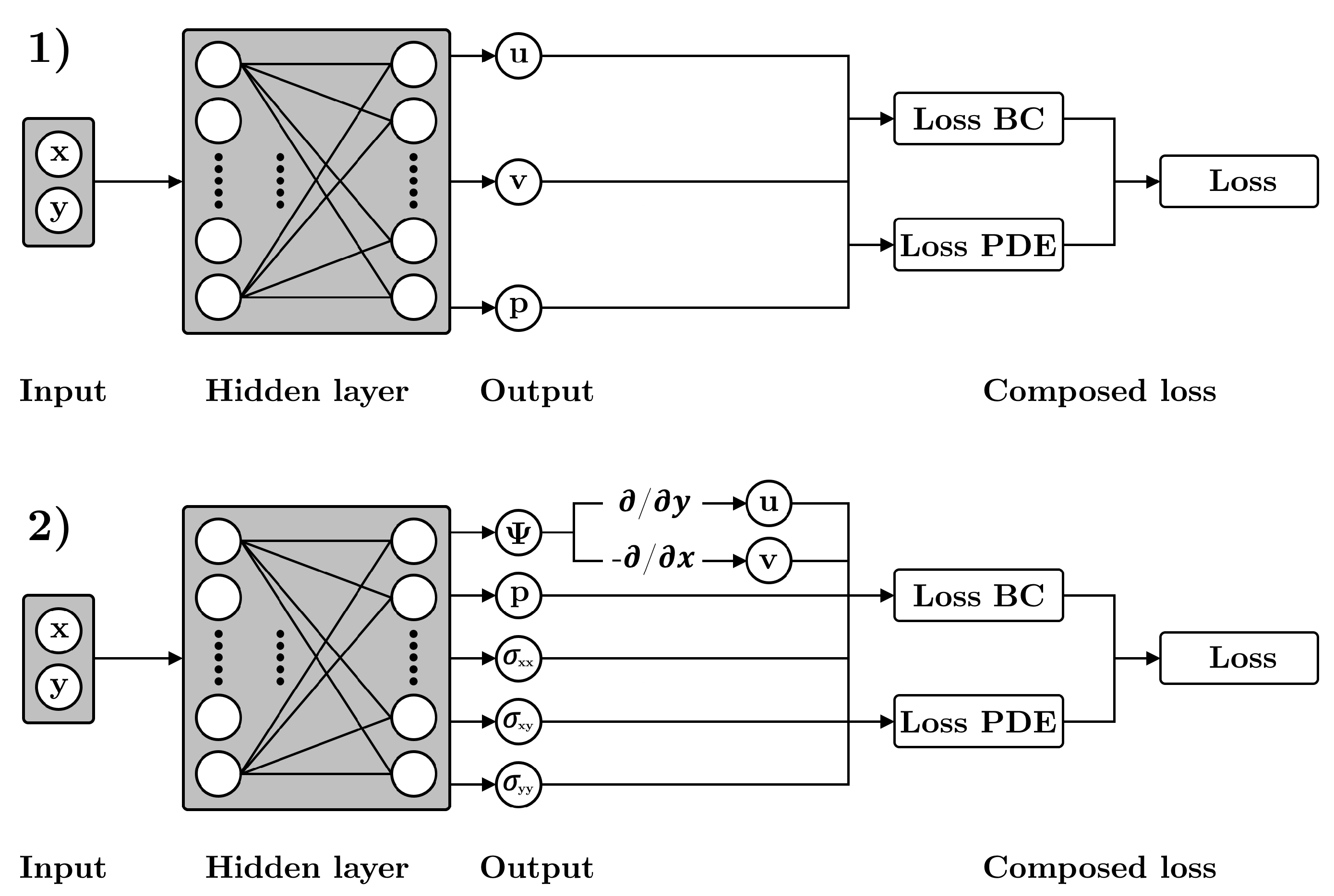
where ∇ is the Nabla operator. A feedforward NN was trained to predict

ψ

, p, and the stress components

σ_{x x}

σ_{x y} = σ_{y x}

, and

σ_{y y}

. The network takes the coordinates x and y as inputs and passes the velocity components, the pressure, and the stress components back. The model reads as follows:

N N_{θ} (\begin{matrix} x \\ y \end{matrix}) = (\begin{matrix} ψ \\ p \\ σ_{x x} \\ σ_{x y} \\ σ_{y y} \end{matrix})

(19)

In agreement with equations (15) to (17), the residuals

ε_{k}

are computed as

\begin{matrix} ↑_{k = 1, 2} = \bar{u_{j}} \frac{\partial \bar{u_{i}}}{\partial x_{j}} - \frac{\partial σ_{i j}}{\partial x_{j}} \end{matrix}

(20)

↑_{k = 3, 4, 5} = - p + μ_{r e s} (\frac{\partial \bar{u_{i}}}{\partial x_{j}} + \frac{\partial \bar{u_{j}}}{\partial x_{i}}) - σ_{i j}

(21)

↑_{k = 6} = p + \frac{1}{2} σ_{i i}

(22)

For the traditional approach, the two input neurons were fed into a single fully connected feed-forward network with three output neurons as determined by Equation (12). For the mixed-variable approach, the two input neurons were fed into a single fully connected feed-forward network with five output neurons as defined by Equation (19). Figure 2 shows the two methods that were compared here.

For all networks, a tanh activation function was deployed. In a first step, the PINNs were trained using the Adam optimizer for 100,000 iterations with a decaying learning rate. The initial learning rate was set to 0.001 and was reduced by a factor of 0.9 every 2,000 iterations. In a second step, the models were trained using the L-BFGS optimizer under the predefined default settings. No loss weigthing factors were defined. The training was conducted using the tensorflow-based library DeepXDE [22].

2.3. Reference data

The capability of the PINN to represent the solution of the RANS equations under consideration of the mixing length model was evaluated and compared with CFD simulations for geometries G1 and G2. For the CFD calculations, the element-based finite volume flow solver MAYA included in the Simcenter software was used. The MAYA solver provided the mixing length model with Van Driest damping. Unstructured meshes featuring prism layers on the cylinders were defined. The second order upwind discretization scheme was deployed. The incompressible calculations were carried out until reaching the minimal achievable residuals. A grid sensitivity analysis was carried out to verify the models. For the grid study, three grids were generated using a refinement factor of 1.3. Excellent agreement between all three grids was found and, consequently, the reference solution was concluded to be grid independent.

The PINN predictions for geometry G3 were compared with experimental results of Lyn et al. [20] who conducted two-component laser-Doppler measurements for a square cylinder inside a closed water channel at a Reynolds number of

2.14 \times 10^{4}

. The time averaged data were obtained from the ERCOFTAC validation database [23].

2.4. Study design

This study, comprising three parts, compared the traditional method with the mixed-variable method, investigated effects of network shape and size for different geometries, and compared the predictions with measurements. For both PINN methods, several network architectures were compared. The network sizes were chosen to yield the same number

N_{θ}

of trainable parameters

θ

(weights and biases) inside the network, where

N_{θ}

is defined as follows:

N_{θ} = N_{i n} N_{n} + N_{n}^{2} (N_{l} - 1) + N_{o u t} N_{n} + N_{n} N_{l}

(23)

Here,

N_{o u t}

represents the number of output neurons and

N_{i n}

the number of input neurons. The number of neurons per layer,

N_{n}

, and the number of hidden layers,

N_{l}

, were set to yield a progressing series of shape factor values,

λ

. The shape factor was defined as follows:

λ = \frac{N_{n}}{N_{l}}

(24)

A low value of

λ

represented a deep but narrow network architecture featuring comparatively few neurons per layer and many hidden layers. An elevated result for

λ

corresponded to a shallow but wide network consisting of a high amount of neurons per layer and few hidden layers.

In the first part of our study, the traditional method was tested using geometry G1. This part documented limitations of the traditional PINN method when applied to high Reynolds number flows. Table 2 lists the tested networks of the first part.

In the second part, the best fitting network shapes and sizes for mixed-variable PINN models were evaluated and the results for geometry G1 and G2 were compared. The purpose of this part was to find appropriate network shapes, outline differences between the two geometries, and document capabilities and limitations of unsupervised mixed-variable models when applied to high Reynolds number flows. A total of five network architectures were deployed with corresponding shape factors ranging from

4.08 \times 10^{- 1}

1.34 \times 10^{2}

. Table 3 lists the evaluated networks.

Furthermore, after selecting the network shapes giving the most accurate results, several networks featuring a constant shape factor and a progressing number of trainable parameters

θ

were defined and tested. Different shape factors were chosen for the circular cylinder and the square cylinder. Table 4 lists the networks evaluated in the second step.

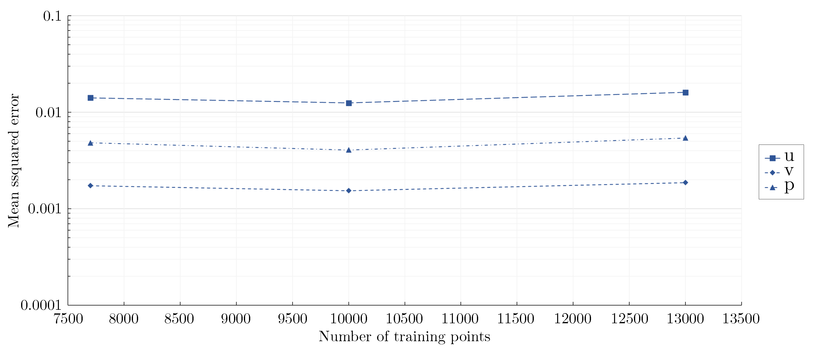
10,000 randomly distributed training points were used on the boundaries as well as inside the flow domain for geometries G1 and G2. This represented 1,250 points per m² of the flow domain and 754 points per m of the boundaries. The number of points was evaluated in a prior sensitivity analysis conducted for the circular cylinder G1 using the mixed-variable PINN N50L30. The evaluation revealed no increase in accuracy by increasing the number of points, as shown in Figure 3. The density of points deployed here was 3.87 times greater than used in a study of Ang et al. [21] who reported no change in accuracy beyond 323 points per m² of the scaled flow domain for a laminar flow field.

In the third part, geometry G3 was considered and an unsupervised PINN was compared with the experimental results of Lyn et al. [20]. A search for the most suitable network shape was conducted in the same way as described above for part two. As the general method and behavior of the PINN was equivalent, the detailed results of this study are not presented here. Model N50L30 was identified as the most suitable architecture for geometry G3. The corresponding settings of the network are listed in Table 5. To account for the small scale of the cylindrical body contained in geometry G3, the number of training points inside the domain was increased to 80000. The purpose of this part was to get an impression of the validity of the mixed-variable PINN method when no labeled training data are provided.

3. Results

3.1. Performance of the traditional method

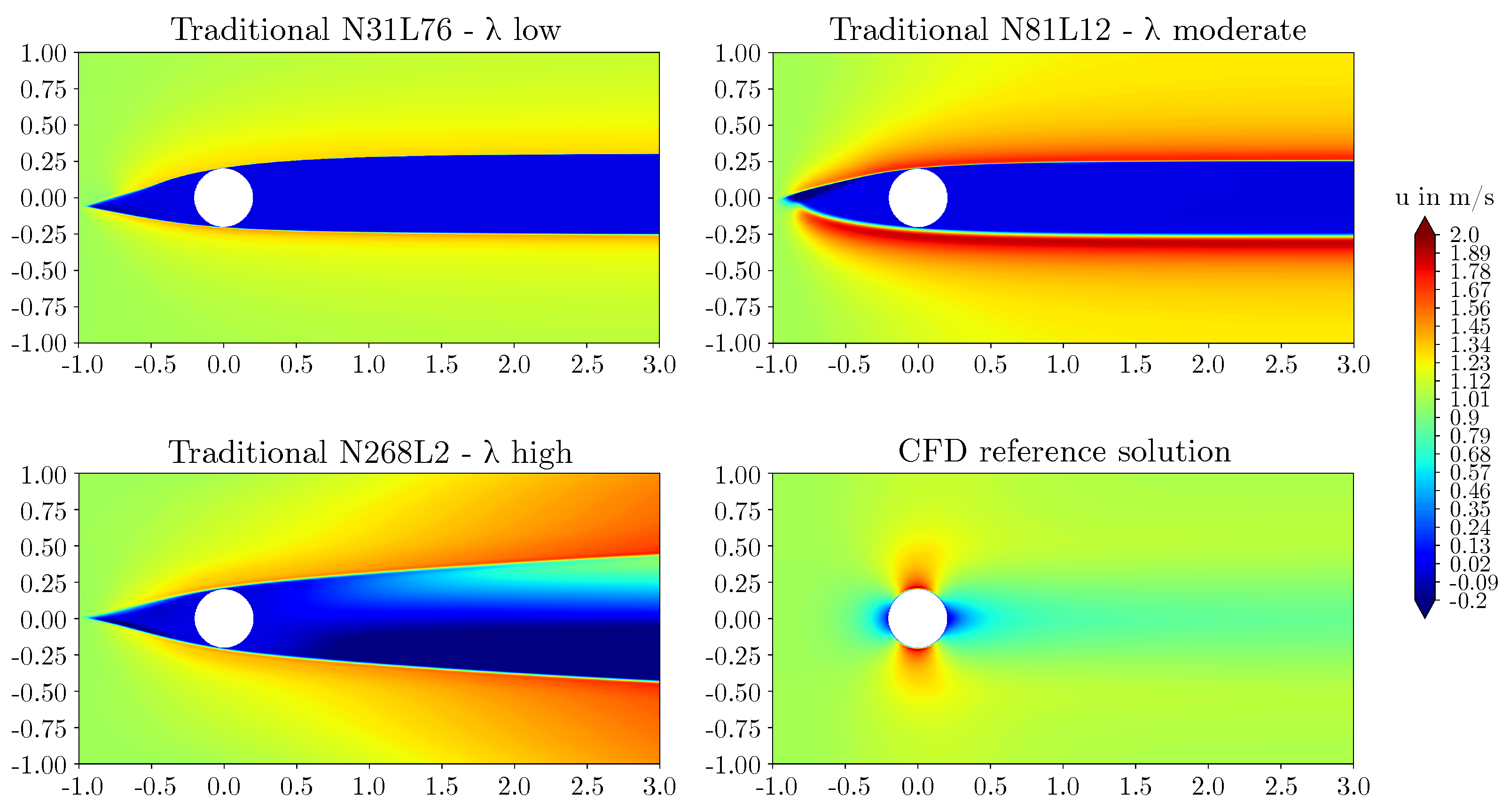
The traditonal PINNs failed to capture the flow field, independent of network architecture. Figure 4 displays comparative predictions for the velocity field around the circular cylinder. As a reference, the CFD results are shown as well. Several models are exhibited that represent high, moderate, and low shape factors. While the flow blockage due to the cylinder was recognized, the flow field was unrealistic and the stagnation region, the flow separation, and the shear layers were not captured correctly. Varying the network shape did not improve the performance of the traditional method.

3.2. Effect of network architecture using the mixed-variable method

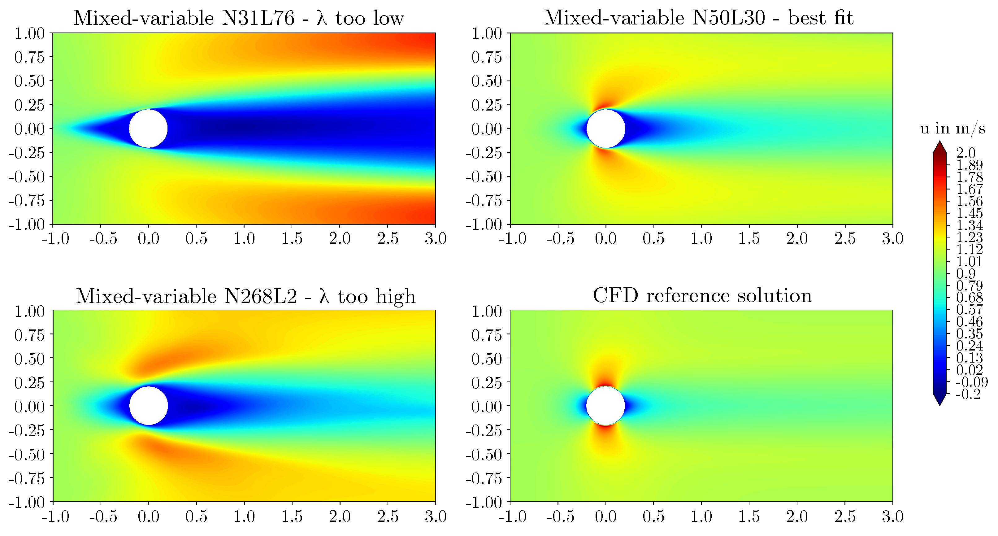
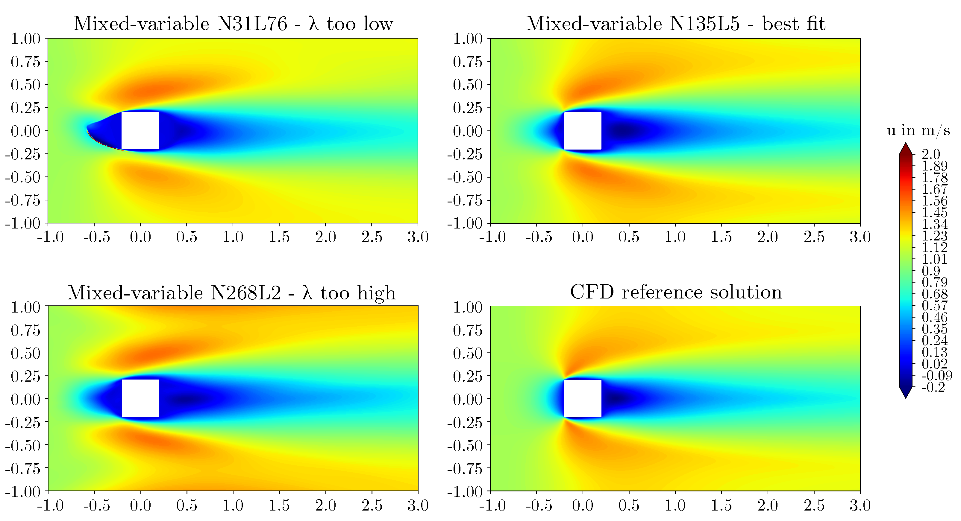
The mixed-variable approach was observed to be sensitive to the network shape. Too deep as well as too wide networks failed to capture the flow field. Figure 5 and Figure 6 display predicted axial velocities of several models together with comparative CFD data. From the shown models, N31L76 and N268L2 represent low and high shape factors, respectively. Both architectures failed to capture the reference flow field accurately. For the circular cylinder, model N50L30 obtained the most accurate predictions, capturing the stagnation region, the thin boundary layer on the cylinder, as well as the wake. However, the wake length was overestimated compared with the reference solution and the high speed region on the lateral sides of the cylinder was deformed. For the square cylinder, model N135L5 exhibited the most accurate results. The stagnation region, the cylinder wake, and the small area of flow separation and recirculation at the lateral sides of the cylinder was captured. However, the size of the low velocity stagnation region upstream of the cylinder was overpredicted when compared with the reference solution.

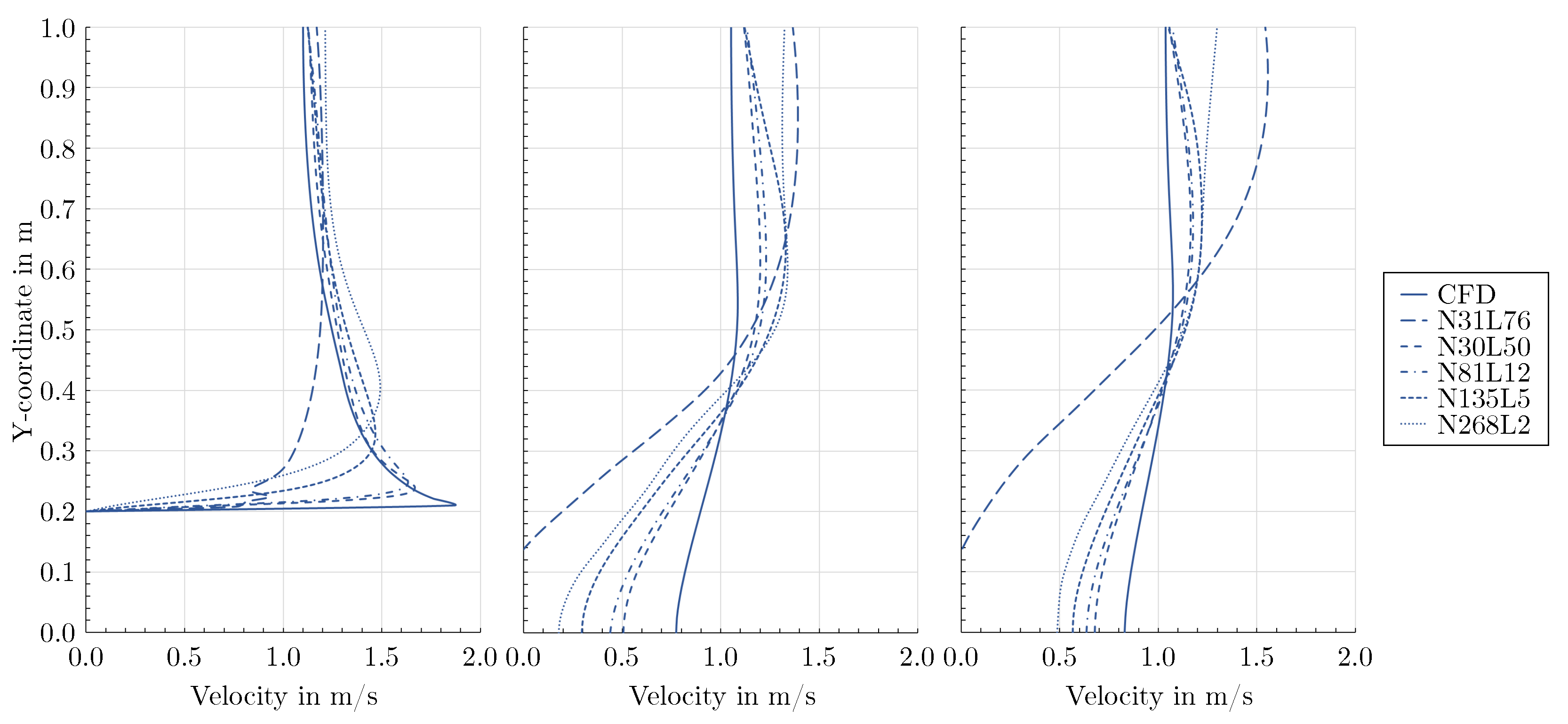
Figure 7 compares axial velocities of the different mixed-variable PINN models with the CFD calculations for the circular cylinder. The results are shown along several vertical lines. At

x = 0

, the high gradients as well as the overshoot of the developing boundary layer were best captured by N50L30 and N81L12. All models predicted a prolonged wake behind the cylinder. This resulted in a greater velocity deficit at

x = 1

m and

x = 2

m, accompanied by a higher free stream velocity at the lateral sides due to volume flow and momentum balances. Model N50L30 captured the reference flow most accurately.

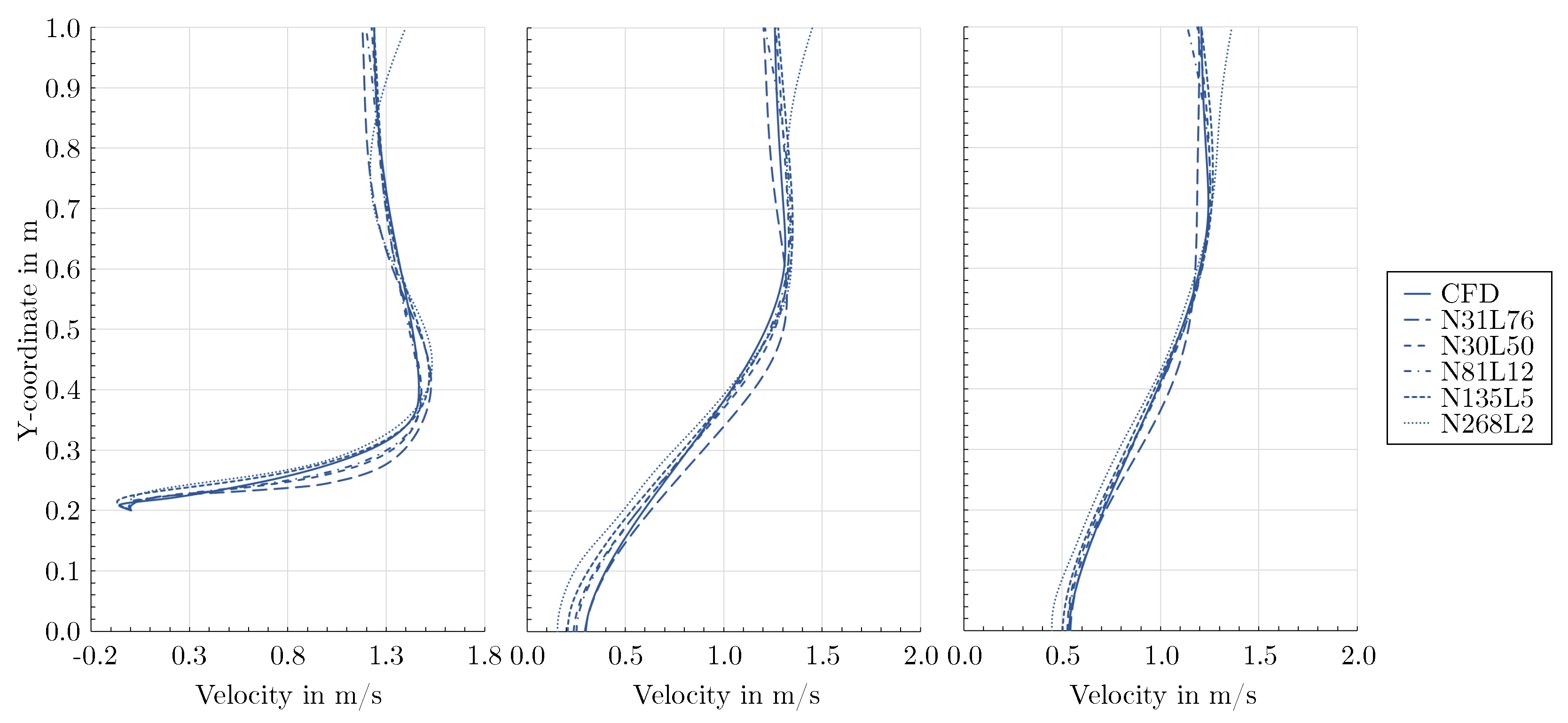
Figure 8 displays the predicted velocity in x-direction along several vertical lines close to the square cylinder. Except for model N268L2, all models showed close agreement. At x=0, model N135L5 accurately captured the recirculating flow on the cylinder surface featured by the reference solution. Furthermore, the velocity overshoot of the developing and separating boundary layer was captured. However, the thickness of the recirculating flow was slightly overestimated and, consequently, the velocity overshoot of the separating boundary layer was overestimated as well. All models accurately predicted the wake behind the square cylinder.

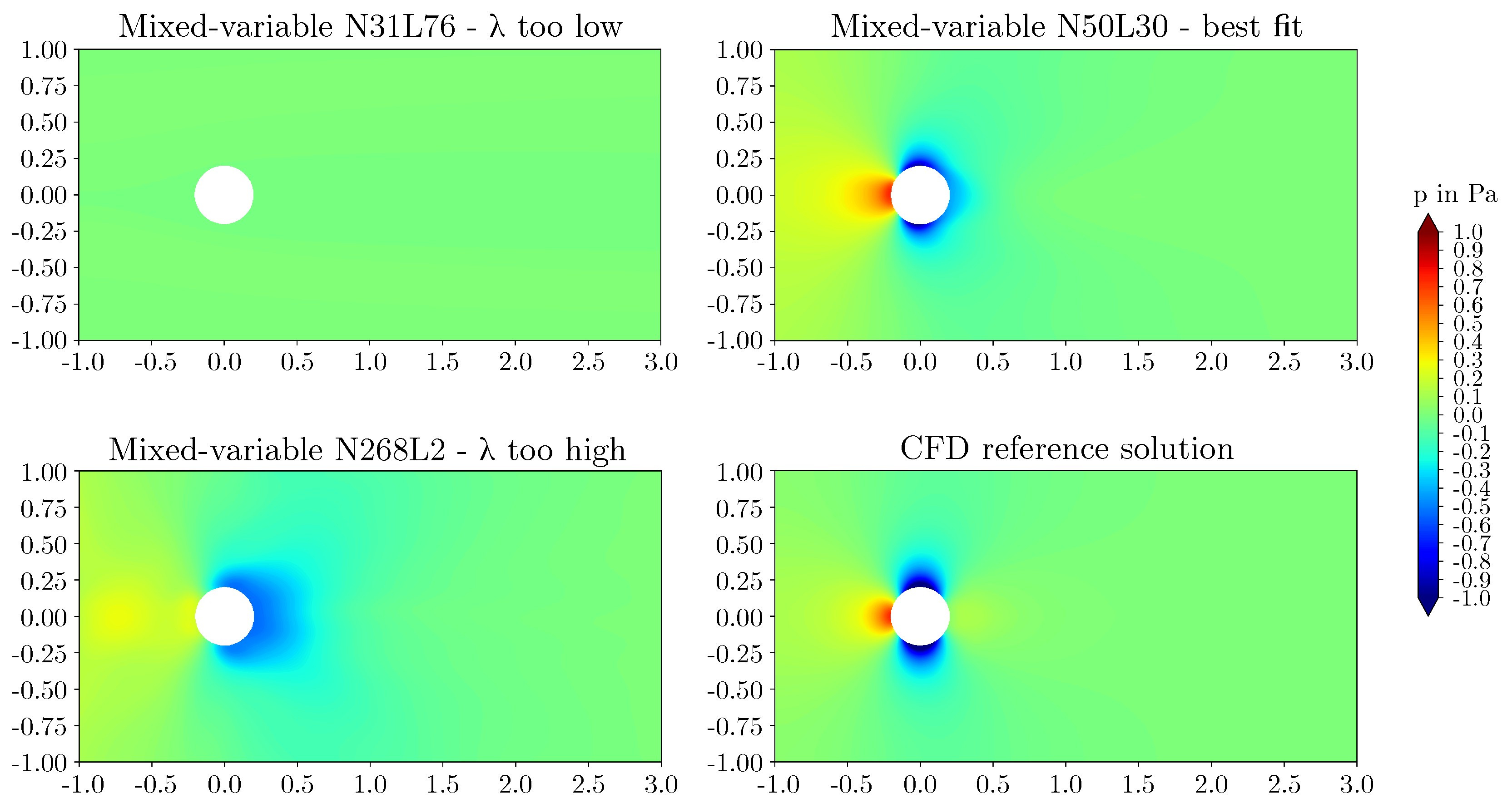
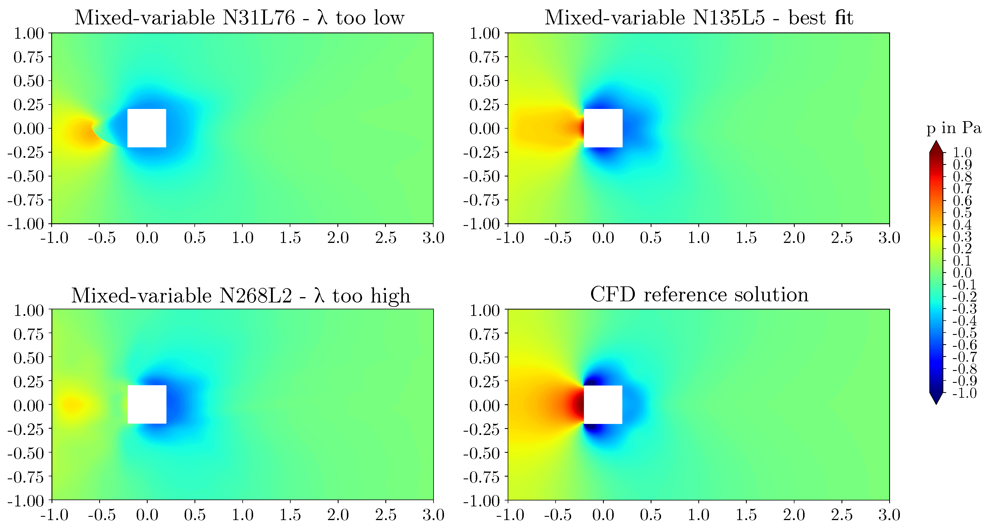
The trends observed for the axial velocity were also observed for the pressure field. Figure 9 and Figure 10 exhibit the pressure predictions and comparative CFD data. For the circular cylinder G1, model N31L76 predicted pressure values close to zero and did not capture the pressure field. For the square cylinder G2, model N31L76 predicted inaccurate results as well. Similarly, model N268L2 did not predict the pressure field accurately. For the circular cylinder, the positive pressure in the stagnation region of the reference solution was underestimated and a moderate negative pressure was predicted around the cylinder. For the square cylinder, model N268L2 predicted a dislocated region of positive pressure at the upstream side of the cylinder. For the circular cylinder, the best fitting model N50L30 captured the positive pressure region at the upwind side of the cylinder as well as the negative pressure at the lateral sides. However, the positive pressure on the downwind side was not predicted. For the square cylinder, the best fitting model N135L5 captured the positive pressure of the stagnation region as well as a negative pressure field around the square cylinder. However, size and magnitude of the positive pressure region as well as the negative pressure region at the upstream corners were underestimated.

The pressure values on the cylinder surface are shown in Figure 11. The deep but narrow model N31L76 predicted a vanishing pressure distribution around the entire cylinder. All models failed to predict the positive pressure region on the downstream side of the cylinder that was present in the CFD reference data. From all mixed-variable models, N50L30 provided the best representation of the reference solution. The minimum pressure peaks were more pronounced and the pressure on the downwind side of the cylinder was increased. Furthermore, the asymmetry associated with the other architectures was reduced.

Figure 12 exhibits a comparison between the pressure distributions on the square cylinder surface. Models N31L76 as well as N268L2 predicted inaccurate results. All other models captured the shift from positive to negative pressure. All networks underestimated the negative pressure maxima at the square edges that were featured by the CFD reference data. Models N50L30 and N81L12 better predicted the sharp shift from positive to negative pressure while model N135L5 more accurately matched the positive pressure magnitude at the upstream side of the square.

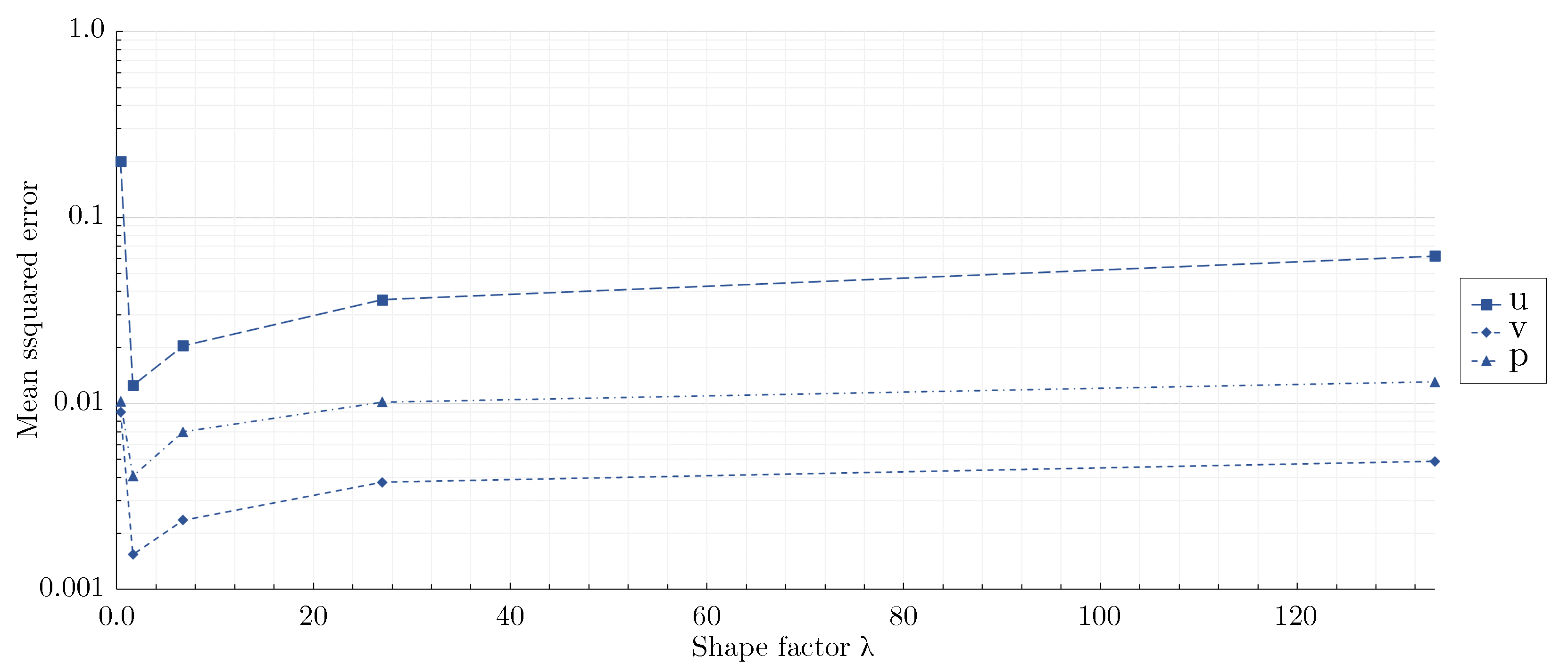
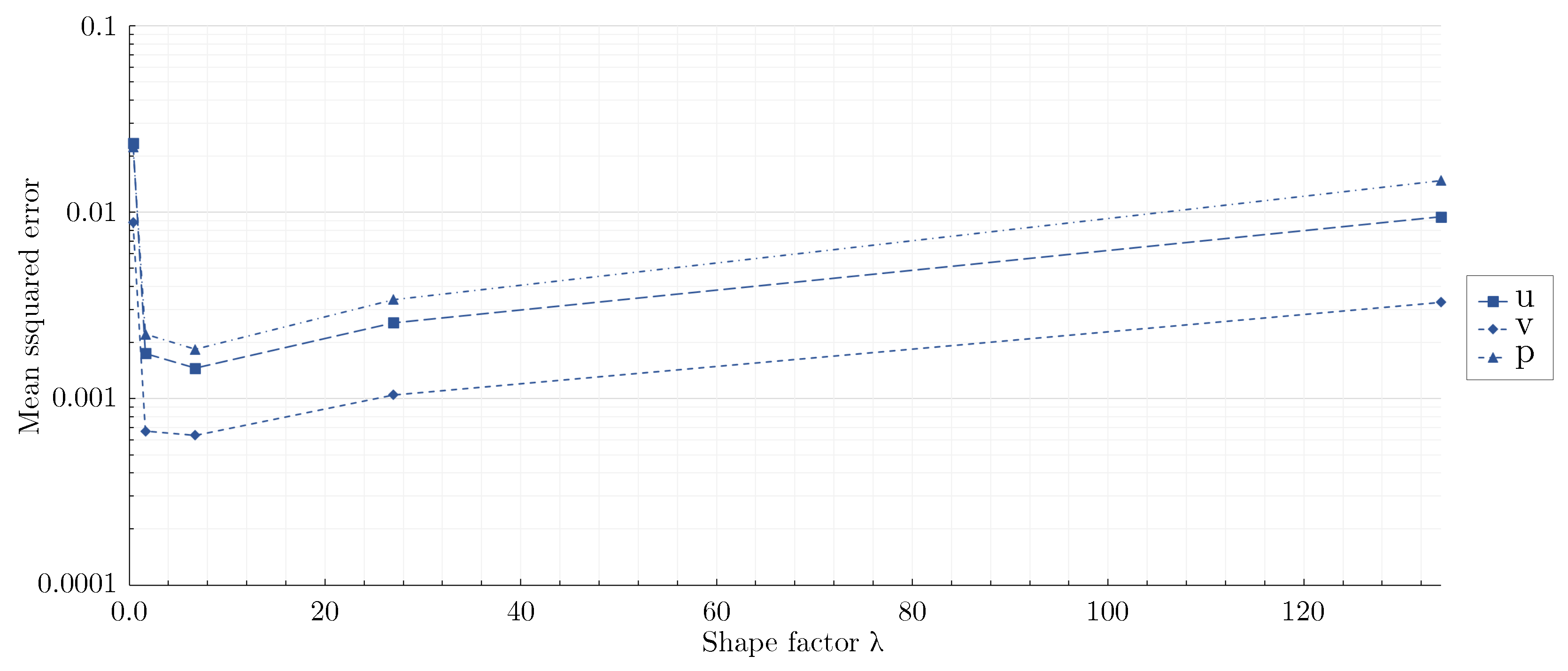
The correlation of shape factor and mean squared error (MSE) is shown in Figure 13 for the circular cylinder G1. As seen, the axial velocity in the x-direction achieved the highest overall MSE. The relationship between MSE and shape factor was similar for all flow field variables. As

λ

tended to zero, the error increased markedly. For the networks with shape factors above

1.67 \times 10^{0}

, the error grew with a decreasing slope. The obtained data suggests an optimal network shape for networks with shape factors close to

1.67 \times 10^{0}

. For the best fitting model, N50L30, the losses for the two momentum equations were

9.23 \times 10^{- 6}

and

6.99 \times 10^{- 6}

for the x- and y-directions, respectively. The achieved losses indicate that the governing equations were satisfied. The correlation between MSE and shape factor was different for the two cylinder geometries. Figure 14 displays the MSE of the different network shapes for the square cylinder G2. As seen, the error tended to a minimum for shape factors between

6.75 \times 10^{0}

and

2.70 \times 10^{1}

. For the square cylinder, the best shape factor was greater than for the circular cylinder. Furthermore, close to its minimum, the growth of the MSE was less and featured a broader region of minimal MSE. However, the models featuring the lowest NMSEs, i.e., N50L30 and N81L12 also featured artificial velocity peaks at the upstream corners of the square and, hence, were discarded. For model N135L5, featuring a shape factor of

2.70 \times 10^{1}

, the achieved losses for the momentum equations were

3.23 \times 10^{- 5}

and

2.47 \times 10^{- 5}

. The minimal global MSEs for u, v, and p were lower for the square cylinder while the corresponding losses of the best model were lower for the circular cylinder.

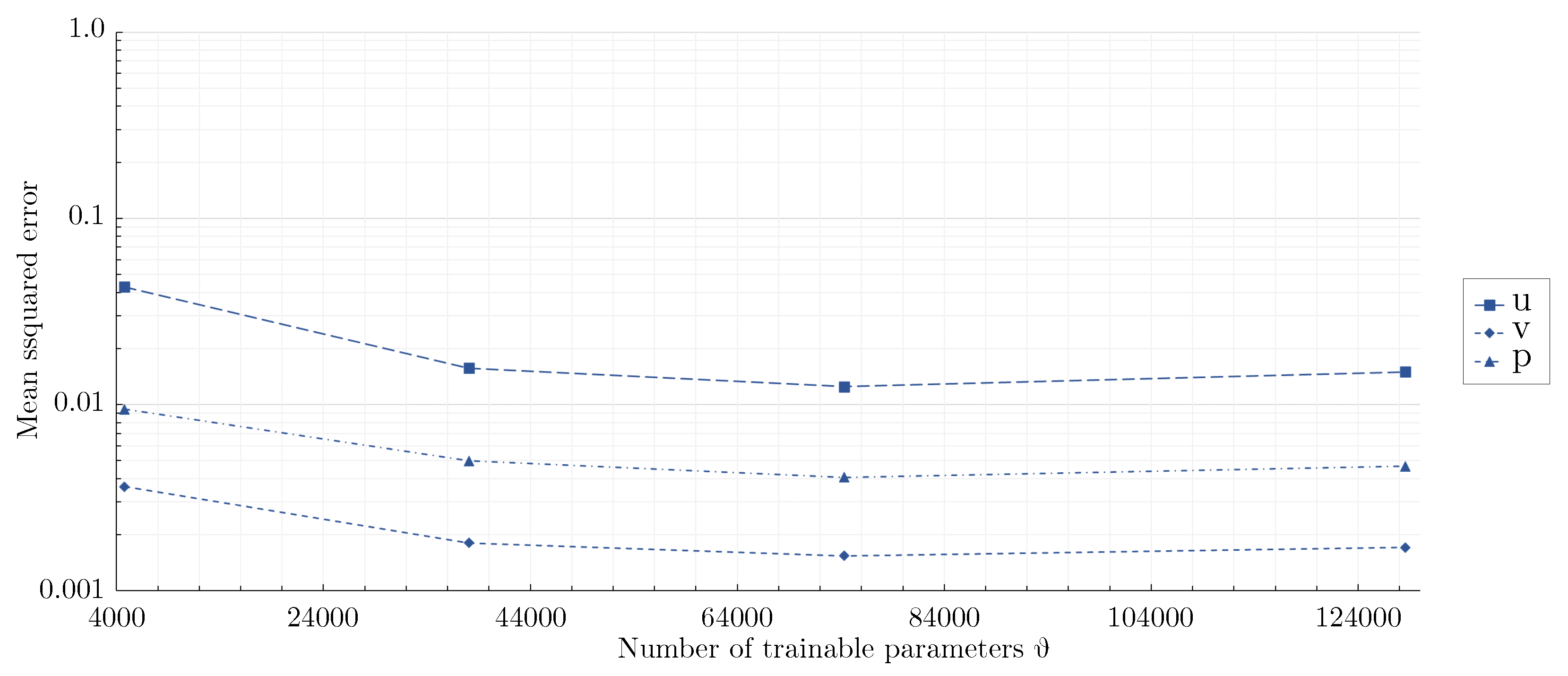
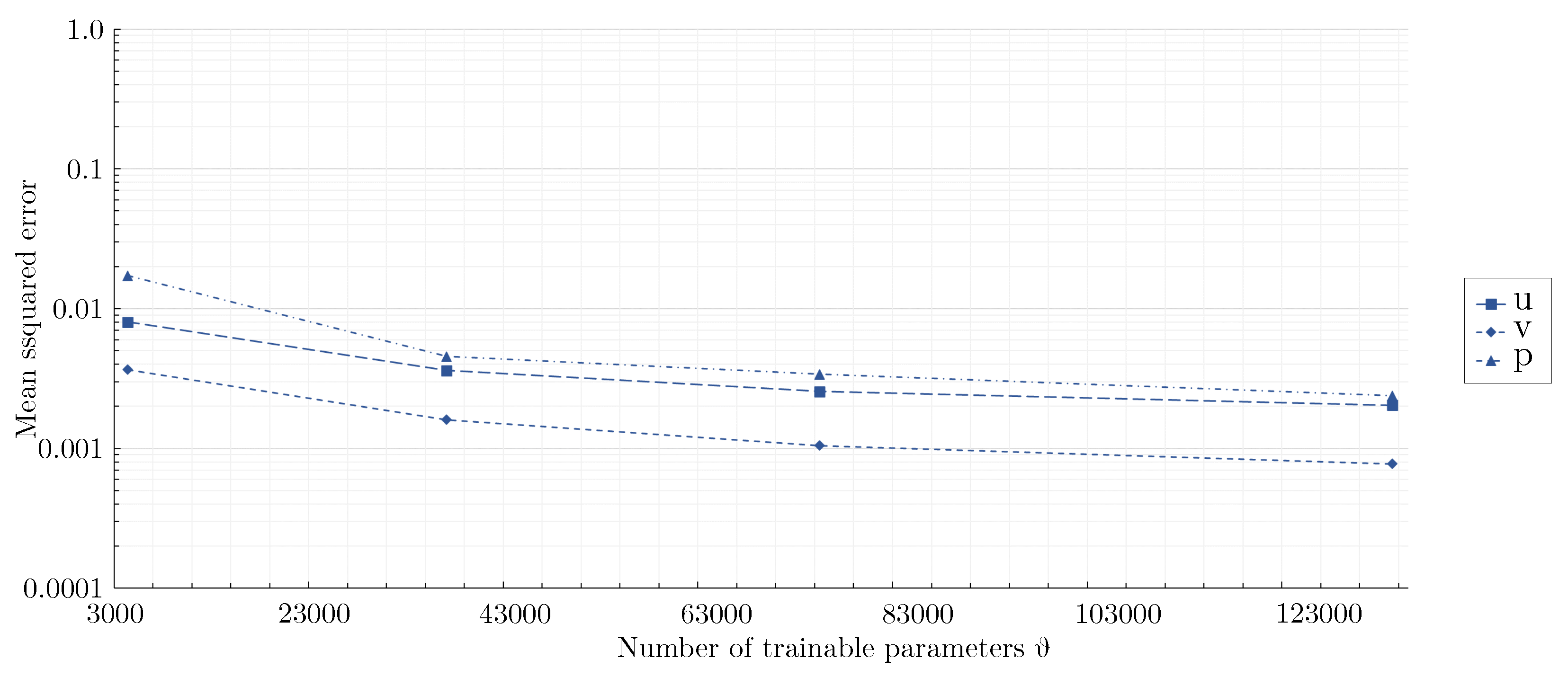
Figure 15 exhibits the MSEs obtained by the different network sizes featuring the best fitting shape factor

1.67 \times 10^{0}

for the circular cylinder. As seen, the network N20L12, featuring 4780 trainable parameters, yielded the greatest errors. The corresponding predictions of the velocity field were inaccurate and comparable to that of model N268L2 shown in Figure 5. The other models, featuring a greater number of trainable parameters, yielded similar errors. Model N50L30, featuring 74350 trainable parameters, was well within the size independent range and neither a reduction nor an increase of the number of trainable parameters led to a further reduction of the global MSE, indicating the superiority of this architecture. Figure 16 exhibits the results of the evaluation of the network size for the square cylinder. In contrast to the circular cylinder, the global MSEs decreased over the entire range of tested network sizes. For model N54L2, featuring 3402 trainable parameters, the highest errors were recorded, and the corresponding predictions were comparable to that of model N31L76 shown in Figure 6. Increasing the number of trainable parameters from 74,520 to 133,326 led to a reduction of 20-30% of the global NMSE for model N162L6. However, the predictions showed no qualitative improvement and featured artificial velocity peaks at the upstream corners of the square. Hence, the larger model did not lead to more favorable predictions of the flow field.

3.3. Validation of the mixed-variable method against measurements

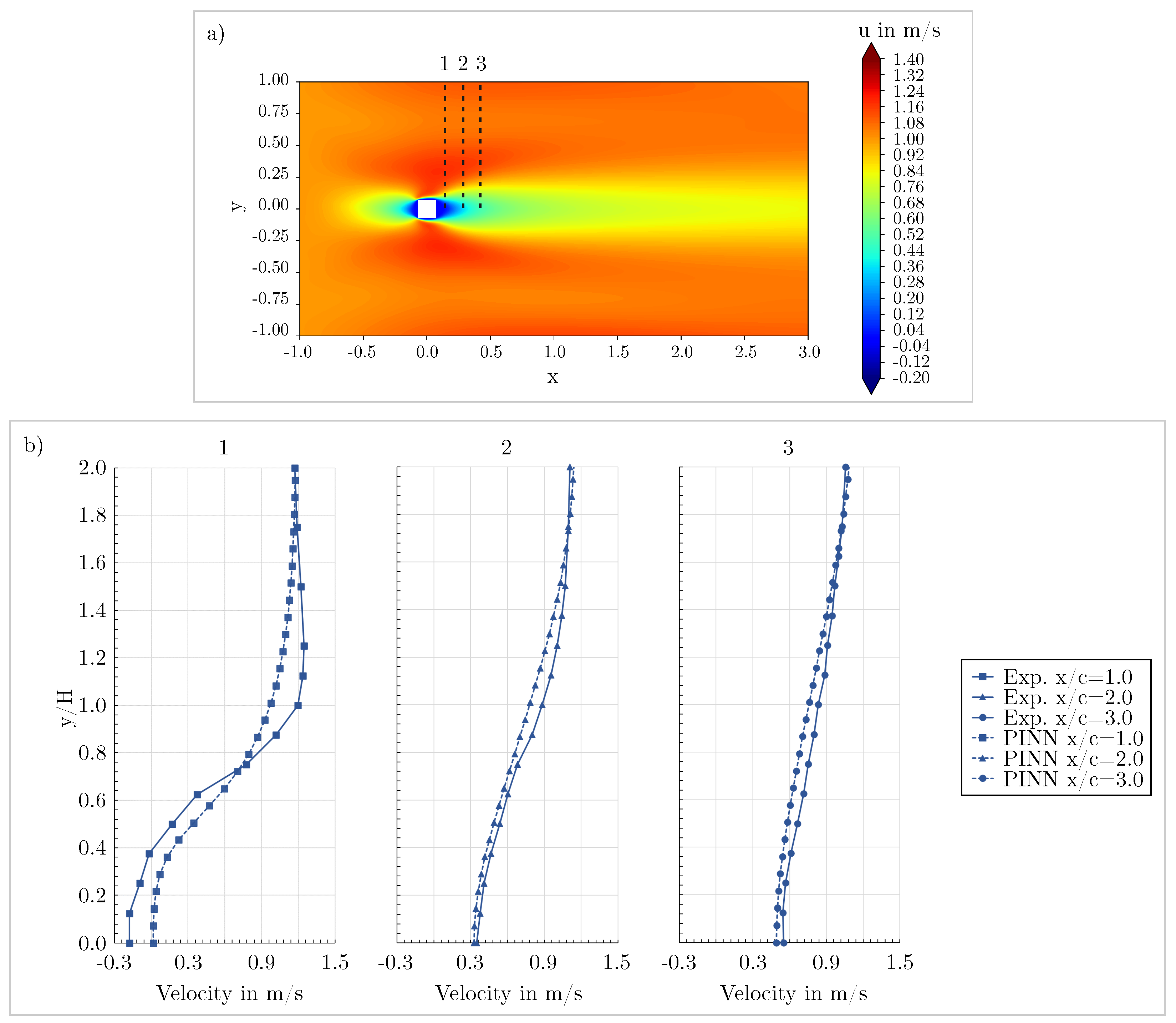
Figure 17 a) exhibits the axial velocity field for geometry G3 as predicted by model N81L12. As seen, the PINN captured a stagnation region of lower velocity at the upwind edge of the square as well as a wake at the downwind side of the cylinder. Furthermore, the high velocity areas extending from the upwind corners of the square were captured. Overall, the flow field was well captured. A comparison of the axial velocity as predicted by the PINN and the values obtained from the time averaged laser-Doppler measurements is shown in Figure 17 b) for several vertical lines in the wake of the square cylinder. In the PINN predictions, the velocity deficit inside the wake was less pronounced at

x / c = 1.0

and, due to momentum and mass conservation, a lower velocity was predicted at the outer extent of the shear layer at

y / c = 1.0

. Overall, there was a favorable agreement between the PINN predictions and the measured results, considering the small scale of the cylinder and the absence of any simulated or measured data during training of the neural net.

4. Discussion

The traditional PINNs failed to yield acceptable predictions for the elevated Reynolds number flow investigated here. For lower Reynolds number flows, successful training was reported by Ang et al. [21]. A major challenge of high Reynolds number flows is the increasing complexity of the optimization problem as the nonlinear convective momentum terms of the RANS equations become dominant, shear leayer gradients become steeper, and turbulence models increase the complexity of the RANS equations. Utilizing the mixed-variable approach advanced the training success of the PINN method. However, due to the complexity of the optimization problem, there were still deviations from the reference solution. This contrasts the excellent results of Rao et al. [19], obtained for a laminar low Reynolds number flow. Increasing errors associated with higher Reynolds numbers were also reported by Sun et al. [8] and Harmening et al. [12]. Consequently, numerous studies were conducted incorporating measured or simulated training data to support training of the PINN [14,15,16,17,18,24,25,26], while investigations focusing unsupervised physics-informed DL of high Reynolds number flows without training data remain sparse [13].

For the circular cylinder G1, the high gradients of the flow were not successfully learned by most network architectures. Only models N50L30 and N81L12 captured the boundary layer on the cylinder at x=0. Furthermore, the wake length was predicted more accurately by model N50L30. For the square cylinder G2, models N135L5 and N81L12 exhibited superior performance. The flow separation and recirculation that was present on the lateral sides of the cylinder at

x = 0

was best captured by model N135L5. However, model N81L12 achieved the lowest overall MSE. As the corresponding shape factors varied by up to one order of magnitude, distinct network architectures were necessary to capture the flow fields around the two geometries most accurately. These results imply that networks yielding accurate predictions in certain cases might significantly deviate from networks suitable for other cases. More work is needed to further investigate the best architectures for more complex geometries.

The superiority of the N50L30 architecture to predict the flow around the circular cylinder G1 as well as the square cylinder of geometry G3 agreed favorably with a study of Ang et al. [21], who identified a traditional PINN with 50 neurons per layer and a minimum of 20 hidden layers most suitable for a low Reynolds number flow around a circular cylinder. This corresponds to shape factors below

2.5 \times 10^{0}

. Rao et al. [19] studied a laminar low Reynolds number flow and used a mixed-variable PINN comprising 40 neurons per hidden layer with a total of eight hidden layers. The network featured a shape factor of

5.0 \times 10^{0}

and comprised 15.9% of the trainable parameters contained in the N50L30 model used here. We investigated this architecture in preparation of our study as well; however, the model yielded unfavorable results similar to our models N268L2 or N20L12. Eivazi et. al [17] applied a network architecture of 20 neurons per layer and eight layers using the traditional PINN approach. The shape factor of this model was

2.5 \times 10^{0}

and featured 4.2% of the trainable parameters of the N50L30 model. Eivazi et. al reported good results for fractions of flow fields at elevated Reynolds numbers without using training data in the flow domain. However, for the flow we investigated, the architecture also exhibited unfavorable results similar to the high shape factor model N268L2 or the smaller model N20L12. As discussed above, network architectures and types that proved to be suitable for specific cases can not readily be applied to other cases and, consequently, a comprehensive screening of the best shape and size needs to be carried out.

While preparing this study, methods including non-adaptive loss weighting for the traditional approach, hard boundary constraints [8], vorticity formulation of the RANS equations [9], Helmholtz decomposition [16], residual neural networks, and Fourier feature networks [27] were tested. However, these methods did not exhibit favorable results and, therefore, they are not discussed here in detail. Other turbulence models, such as an equation-free modeling approach [14,17,18], Prandtl’s one equation k model, and the k-

ω

model of Wilcox [28], were tested as well in preparation of this study. However, the traditional turbulence models suffered from stability issues during the training process, while the equation-free approach did not capture the flow field accurately. Applying the mixed-variable approach, considering the mixing length turbulence model in combination with networks featuring proper shape factors and sufficient trainable parameters, was the only method that was capable of capturing the stagnation points, high gradient boundary layers, and flow separation of the investigated high Reynolds number flow fields. Nevertheless, an extensive search for the best network shapes was necessary to obtain these results.

Yet, the effect of the shape factor and the network size on the prediction accuracy was limited. A remaining bias error regarding the wake length behind the circular cylinder, an overestimation of the stagnation region size for the square cylinder, as well as an underestimation of the pressure peaks on the cylinder surfaces was observed, documenting the difficulties associated with predicting high Reynolds number flows using PINNs. Hence, more work is needed to further increase the prediction accuracy of the mixed-variable method. The deviations between the mixed-variable predictions and the CFD reference solution were attributed to optimization errors, generalization errors, and approximation errors. A modeling error concerning the RANS turbulence model also contributed to the differences between the PINN predictions and the measured velocities. As reported by Harmening et al. [12], the network and training related errors could be reduced to a minimum by introducing training data. Other potential methods to improve the accuracy include curriculum learning [29], adaptive loss weighting [27,30,31,32], convolutional or U-Net PINNs [11,33,34,35,36], and distributed PINNs [37], among others. The geometries investigated here should serve as a benchmark case to evaluate such methods because the corresponding high Reynolds number flow fields feature a number of important flow phenomena that any reliable PINN methodology must be capable to capture.

The method investigated here may be used with and without labeled training data. As the mixed-variable approach yielded favorable results without using any training data, the required data quantities to train mixed-variable models agreeing with CFD or experimental studies can be expected to be minimal. The method may be used for improved interpolations and extrapolations between data points. The method without training data can be applied for comparative studies and optimization processes [13]. However, then the demonstrated limitations of the PINN models need be taken into account.

5. Summary and Conclusions

We compared different network architectures using mixed-variable physics-informed deep learning and traditional PINNs with CFD and measured reference data. The models were trained to solve the two-dimensional RANS equations for a turbulent flow around a circular cylinder and a square cylinder. The mixing length turbulence model was deployed. The main findings are summarized as follows:

For the elevated Reynolds number flow considered here, the superiority of the mixed-variable approach of Rao et al. [19] was confirmed. The traditional PINN method failed to capture the flow field accurately, independent of the network architecture.
For the flow around the large scale circular cylinder, the deep architecture with a shape factor of $1.67 \times 10^{0}$ outperformed the other architectures. The steep gradients of the boundary layers were predicted more accurately and the prolonged wake was reduced. For the flow around the large scale square cylinder, the wide network with a shape factor of $2.70 \times 10^{1}$ captured the reference solution best. The model with a shape factor of $6.75 \times 10^{0}$ worked well for both geometries.
For the geometries investigated, different mixed-variable network architectures with factors varying by one order of magnitude were suitable. This demonstrates that depending on the case, it might be necessary to distinctly vary the shape factor of a PINN to find the best fitting model. However, using extremely high or low shape factors proved to be inappropriate.
Despite inevitable deviations from the reference flow fields, the physics-informed mixed-variable method applied with a proper network architecture was able to predict stagnation points, high gradient boundary layers, flow separation, recirculation areas, and wakes at an elevated Reynolds number without requiring training data. In contrast, regular neural nets are not capable to predict plausible flow fields without providing extensive training data inside the domain.
The mixing length model proved to be a reliable and stable model for physics-informed deep learning when no simulated or measured data were considered.
More work needs to be done concerning physics-informed deep learning of the RANS equations. Future work should consider other turbulence models and methods to further increase the accuracy of predicted high Reynolds number flows.

Author Contributions

J.H.H.: Conceptualization; Investigation; Methodology; Software; Project administration; Writing – original draft. F.J.P.: Resources; Supervision; Writing – review and editing. O.el M.: Supervision; Writing – review and editing.

Data Availability Statement

The data that support the findings of this study are available from the corresponding authors upon request.

Acknowledgments

We are grateful to Thomas Erling Schellin for review of the manuscript.

Conflicts of Interest

The authors have no conflicts to disclose.

References

Pinkus, A. Approximation theory of the MLP model in neural networks. Acta Numerica 1999, 8, 143–195. [Google Scholar] [CrossRef]
Thuerey, N.; Weißenow, K.; Prantl, L.; Hu, X. Deep Learning Methods for Reynolds-Averaged Navier–Stokes Simulations of Airfoil Flows. AIAA Journal 2020, 58, 25–36. [Google Scholar] [CrossRef]
Lagaris, I.E.; Likas, A.; Fotiadis, D.I. Artificial neural networks for solving ordinary and partial differential equations. IEEE transactions on neural networks 1998, 9, 987–1000. [Google Scholar] [CrossRef]
Raissi, M.; Perdikaris, P.; Karniadakis, G.E. Physics Informed Deep Learning (Part I): Data-driven Solutions of Nonlinear Partial Differential Equations, 2017. Preprint at http://arxiv.org/pdf/1711.10561v1.
Raissi, M.; Perdikaris, P.; Karniadakis, G.E. Physics Informed Deep Learning (Part II): Data-driven Discovery of Nonlinear Partial Differential Equations, 2017. Preprint at http://arxiv.org/pdf/1711.10566v1.
Raissi, M.; Perdikaris, P.; Karniadakis, G.E. Physics-informed neural networks: A deep learning framework for solving forward and inverse problems involving nonlinear partial differential equations. Journal of Computational Physics 2019, 378, 686–707. [Google Scholar] [CrossRef]
Raissi, M.; Yazdani, A.; Karniadakis, G.E. Hidden fluid mechanics: Learning velocity and pressure fields from flow visualizations. Science (New York, N.Y.) 2020, 367, 1026–1030. [Google Scholar] [CrossRef]
Sun, L.; Gao, H.; Pan, S.; Wang, J.X. Surrogate modeling for fluid flows based on physics-constrained deep learning without simulation data. Computer Methods in Applied Mechanics and Engineering 2020, 361, 112732. [Google Scholar] [CrossRef]
Jin, X.; Cai, S.; Li, H.; Karniadakis, G.E. NSFnets (Navier-Stokes Flow nets): Physics-informed neural networks for the incompressible Navier-Stokes equations. Journal of Computational Physics 2021, 426, 109951. [Google Scholar] [CrossRef]
Laubscher, R.; Rousseau, P. Application of a mixed variable physics-informed neural network to solve the incompressible steady-state and transient mass, momentum, and energy conservation equations for flow over in-line heated tubes. Applied Soft Computing 2022, 114, 108050. [Google Scholar] [CrossRef]
Ma, H.; Zhang, Y.; Thuerey, N.; Hu, X.; Haidn, O.J. Physics-driven Learning of the Steady Navier-Stokes Equations using Deep Convolutional Neural Networks, 2021. Preprint at http://arxiv.org/pdf/2106.09301v1.
J. H. Harmening.; F. Pioch.; L. Fuhrig.; F.-J. Peitzmann.; D. Schramm.; O. el Moctar. Data-Assisted Training of a Physics-Informed Neural Network to Predict the Reynolds-Averaged Turbulent Flow Field around a Stalled Airfoil under Variable Angles of Attack 2023. Preprint at https://www.preprints.org/manuscript/202304.1244/v1. [CrossRef]
Hennigh, O.; Narasimhan, S.; Nabian, M.A.; Subramaniam, A.; Tangsali, K.; Fang, Z.; Rietmann, M.; Byeon, W.; Choudhry, S. NVIDIA SimNet™: An AI-Accelerated Multi-Physics Simulation Framework. In Computational Science – ICCS 2021; Paszynski, M., Kranzlmüller, D., Krzhizhanovskaya, V.V., Dongarra, J.J., Sloot, P.M., Eds.; Springer International Publishing: Cham, 2021; Vol. 12746, Lecture Notes in Computer Science; pp. 447–461. [Google Scholar] [CrossRef]
Pioch, F.; Harmening, J.H.; Müller, A.M.; Peitzmann, F.J.; Schramm, D.; el Moctar, O. Turbulence Modeling for Physics-Informed Neural Networks: Comparison of Different RANS Models for the Backward-Facing Step Flow. Fluids 2023, 8, 43. [Google Scholar] [CrossRef]
Ghosh, S.; Chakraborty, A.; Brikis, G.O.; Dey, B. RANS-PINN based Simulation Surrogates for Predicting Turbulent Flows 2023. Preprint at https://arxiv.org/pdf/2306.06034.pdf.
Patel, Y.; Mons, V.; Marquet, O.; Rigas, G. Turbulence model augmented physics informed neural networks for mean flow reconstruction, 2023. Preprint at http://arxiv.org/pdf/2306.01065v1.
Eivazi, H.; Tahani, M.; Schlatter, P.; Vinuesa, R. Physics-informed neural networks for solving Reynolds-averaged Navier–Stokes equations. Physics of Fluids 2022, 34, 075117. [Google Scholar] [CrossRef]
Xu, H.; Zhang, W.; Wang, Y. Explore missing flow dynamics by physics-informed deep learning: The parameterized governing systems. Physics of Fluids 2021, 33, 095116. [Google Scholar] [CrossRef]
C. Rao.; H. Sun.; Y. Liu. Physics-informed deep learning for incompressible laminar flows. Theoretical and Applied Mechanics Letters 2020, 10, 207–212. [CrossRef]
Lyn, D.A.; Einav, S.; Rodi, W.; Park, J.H. A laser-Doppler velocimetry study of ensemble-averaged characteristics of the turbulent near wake of a square cylinder. Journal of Fluid Mechanics 1995, 304, 285–319. [Google Scholar] [CrossRef]
Ang, E.H.W.; Wang, G.; Ng, B.F. Physics-Informed Neural Networks for Low Reynolds Number Flows over Cylinder. Energies 2023, 16. [Google Scholar] [CrossRef]
Lu, L.; Meng, X.; Mao, Z.; Karniadakis, G.E. DeepXDE: A deep learning library for solving differential equations. SIAM Review 2021, 63, 208–228. [Google Scholar] [CrossRef]
European Research Community on Flow, Turbulence and Combustion. Classic Collection Database: Case043 (Vortex Shedding Past Square Cylinder). http://cfd.mace.manchester.ac.uk/ercoftac/doku.php?id=cases:case043. [Online; accessed 07.12.2023].
Huang, W.; Zhang, X.; Zhou, W.; Liu, Y. Learning time-averaged turbulent flow field of jet in crossflow from limited observations using physics-informed neural networks. Physics of Fluids 2023, 35. [Google Scholar] [CrossRef]
Kag, V.; Seshasayanan, K.; Gopinath, V. Physics-informed data based neural networks for two-dimensional turbulence. Physics of Fluids 2022, 34. [Google Scholar] [CrossRef]
Xiao, M.J.; Yu, T.C.; Zhang, Y.S.; Yong, H. Physics-informed neural networks for the Reynolds-Averaged Navier–Stokes modeling of Rayleigh–Taylor turbulent mixing. Computers & Fluids 2023, 266, 106025. [Google Scholar] [CrossRef]
Wang, S.; Sankaran, S.; Wang, H.; Perdikaris, P. An Expert’s Guide to Training Physics-informed Neural Networks, 2023. Preprint at https://arxiv.org/pdf/2308.08468.pdf.
Wilcox, D.C. Reassessment of the scale-determining equation for advanced turbulence models. AIAA Journal 1988, 26, 1299–1310. [Google Scholar] [CrossRef]
Krishnapriyan, A.; Gholami, A.; Zhe, S.; Kirby, R.; Mahoney, M.W. Characterizing possible failure modes in physics-informed neural networks. Advances in Neural Information Processing Systems; M. Ranzato.; A. Beygelzimer.; Y. Dauphin.; P.S. Liang.; J. Wortman Vaughan., Eds. Curran Associates, Inc, 2021, Vol. 34, pp. 26548–26560.
Xiang, Z.; Peng, W.; Liu, X.; Yao, W. Self-adaptive loss balanced Physics-informed neural networks. Neurocomputing 2022, 496, 11–34. [Google Scholar] [CrossRef]
Li, S.; Feng, X. Dynamic Weight Strategy of Physics-Informed Neural Networks for the 2D Navier-Stokes Equations. Entropy 2022, 24. [Google Scholar] [CrossRef] [PubMed]
Wang, H.; Liu, Y.; Wang, S. Dense velocity reconstruction from particle image velocimetry/particle tracking velocimetry using a physics-informed neural network. Physics of Fluids 2022, 34, 017116. [Google Scholar] [CrossRef]
Kim, Y.; Choi, Y.; Widemann, D.; Zohdi, T. A fast and accurate physics-informed neural network reduced order model with shallow masked autoencoder. Journal of Computational Physics 2022, 451, 110841. [Google Scholar] [CrossRef]
Zhu, Y.; Zabaras, N.; Koutsourelakis, P.S.; Perdikaris, P. Physics-Constrained Deep Learning for High-dimensional Surrogate Modeling and Uncertainty Quantification without Labeled Data. Journal of Computational Physics 2019, 394, 56–81. [Google Scholar] [CrossRef]
Wang, R.; Kashinath, K.; Mustafa, M.; Albert, A.; Yu, R. Towards Physics-informed Deep Learning for Turbulent Flow Prediction. In Proceedings of the 26th ACM SIGKDD International Conference on Knowledge Discovery & Data Mining; Gupta, R., Liu, Y., Shah, M., Rajan, S., Tang, J., Prakash, B.A., Eds.; ACM: New York, NY, USA, 08232020; pp. 1457–1466. [Google Scholar] [CrossRef]
Wandel, N.; Weinmann, M.; Klein, R. Teaching the Incompressible Navier-Stokes Equations to Fast Neural Surrogate Models in 3D. Physics of Fluids 2021, 33, 047117. [Google Scholar] [CrossRef]
Dwivedi, V.; Parashar, N.; Srinivasan, B. Distributed physics informed neural network for data-efficient solution to partial differential equations, 2019. Preprint at http://arxiv.org/pdf/1907.08967v1.

Figure 1. Geometries of the circular cylinder (left) and the square cylinder (right).

Figure 2. Tested physics-informed deep learning methods. 1) Traditional fully-connected feed-forward architecture; 2) Mixed-variable fully connected feed-forward architecture.

Figure 3. Global mean squared errors obtained for the large scale circular cylinder G1 using different quantities of training points. For visualization purposes, the data points are connected by straight lines.

Figure 4. Predicted axial velocities around the circular cylinder obtained by the traditional PINN method.

Figure 5. Predicted axial velocities around the circular cylinder obtained from the mixed-variable PINN method.

Figure 6. Predicted axial velocities around the square cylinder obtained from the mixed-variable PINN method.

Figure 7. Axial velocities for the circular cylinder at x = 0 m (left), x = 1 m (middle), and x = 2 m (right).

Figure 8. Axial velocities for the square cylinder at x = 0 m (left), x = 1 m (middle), and x = 2 m (right).

Figure 9. Predicted pressure around the circular cylinder obtained by the mixed-variable PINN method.

Figure 10. Predicted pressure around the square cylinder obtained by the mixed-variable PINN method.

Figure 11. Pressure distributions on the circular cylinder surface.

Figure 12. Pressure distributions on the square cylinder surface.

Figure 13. Global mean squared errors for the circular cylinder obtained by the tested mixed-variable network architectures featuring progressing shape factors. For visualization purposes, the data points are connected by straight lines.

Figure 14. Global mean squared errors for the square cylinder obtained by the tested mixed-variable network architectures featuring progressing shape factors. For visualization purposes, the data points are connected by straight lines.

Figure 15. Global mean squared errors for the circular cylinder obtained by the mixed-variable network architectures featuring a constant shape factor of

1.67 \times 10^{0}

and a progressing number of trainable parameters. For visualization purposes, the data points are connected by straight lines.

Figure 15. Global mean squared errors for the circular cylinder obtained by the mixed-variable network architectures featuring a constant shape factor of

1.67 \times 10^{0}

and a progressing number of trainable parameters. For visualization purposes, the data points are connected by straight lines.

Figure 16. Global mean squared errors for the square cylinder obtained by the mixed-variable network architectures featuring a constant shape factor of

2.70 \times 10^{1}

and a progressing number of trainable parameters. For visualization purposes, the data points are connected by straight lines.

Figure 16. Global mean squared errors for the square cylinder obtained by the mixed-variable network architectures featuring a constant shape factor of

2.70 \times 10^{1}

and a progressing number of trainable parameters. For visualization purposes, the data points are connected by straight lines.

Figure 17. Predicted axial velocities compared with experimental results for geometry G3. A) Contour plot of the predicted velocity obtained by the mixed-variable PINN; b) Comparison with experimental data along several vertical lines in the wake of the square cylinder.

Table 1. Parameters of the investigated geometries.

Label	Cylinder shape	Cylinder size H	Blockage ratio	Reference data	Reynolds number	Objective
G1	Circular	0.40 m	20%	CFD	$4.00 \times 10^{5}$	Network study
G2	Square	0.40 m	20%	CFD	$4.00 \times 10^{5}$	Network study
G3	Square	0.14 m	7%	Experiments	$2.14 \times 10^{4}$	Validation

Table 2. Network architectures using the traditional PINN method evaluated in the first part.

Label	Neurons p. l.	Layers	Shape factor	Parameters	Geometry	Methods
N31L75	31	76	$4.08 \times 10^{- 1}$	74586	G1	Traditional
N81L12	81	12	$6.75 \times 10^{0}$	73548	G1	Traditional
N268L2	268	2	$1.34 \times 10^{2}$	73700	G1	Traditional

Table 3. Network architectures featuring progressive shape factors for the mixed-variable deep learning approach.

Label	Neurons p. l.	Layers	Shape factor	Parameters	Geometry	Methods
N31L75	31	76	$4.08 \times 10^{- 1}$	74648	G1 and G2	Mixed-variable
N50L30	50	30	$1.67 \times 10^{0}$	74350	G1 and G2	Mixed-variable
N81L12	81	12	$6.75 \times 10^{0}$	73710	G1 and G2	Mixed-variable
N135L5	135	5	$2.70 \times 10^{1}$	74520	G1 and G2	Mixed-variable
N268L2	268	2	$1.34 \times 10^{2}$	74236	G1 and G2	Mixed-variable

Table 4. Network architectures featuring progressing numbers of trainable parameters for the mixed-variable deep learning approach under investigation.

Label	Neurons p. l.	Layers	Shape factor	Trainable parameters	Geometry	Methods
N20L12	20	12	$1.67 \times 10^{0}$	4780	G1	Mixed-variable
N40L24	40	24	$1.67 \times 10^{0}$	38040	G1	Mixed-variable
N50L30	50	30	$1.67 \times 10^{0}$	74350	G1	Mixed-variable
N60L36	60	36	$1.67 \times 10^{0}$	128580	G1	Mixed-variable
N54L2	54	2	$2.70 \times 10^{1}$	3402	G2	Mixed-variable
N108L4	108	4	$2.70 \times 10^{1}$	36180	G2	Mixed-variable
N135L5	135	5	$2.70 \times 10^{1}$	74520	G2	Mixed-variable
N162L6	162	6	$2.70 \times 10^{1}$	133326	G2	Mixed-variable

Table 5. Settings used for the validation case.

Label	Neurons p. l.	Layers	Shape factor	Trainable parameters	Geometry	Methods
N50L30	50	30	$1.67 \times 10^{0}$	74350	G3	Mixed-variable

Disclaimer/Publisher’s Note: The statements, opinions and data contained in all publications are solely those of the individual author(s) and contributor(s) and not of MDPI and/or the editor(s). MDPI and/or the editor(s) disclaim responsibility for any injury to people or property resulting from any ideas, methods, instructions or products referred to in the content.

© 2023 by the authors. Licensee MDPI, Basel, Switzerland. This article is an open access article distributed under the terms and conditions of the Creative Commons Attribution (CC BY) license (http://creativecommons.org/licenses/by/4.0/).

Copyright: This open access article is published under a Creative Commons CC BY 4.0 license, which permit the free download, distribution, and reuse, provided that the author and preprint are cited in any reuse.

MDPI Initiatives

Important Links

Choose an area of interest and we will send you notifications of new preprints at your preferred frequency.

Disclaimer

Effect of Network Architecture on Physics-Informed Deep Learning of the Reynolds-Averaged Turbulent Flow Field around Cylinders without Training Data

Abstract

1. Introduction

2. Method

2.1. Geometry

2.2. Governing equations and PINN method

2.3. Reference data

2.4. Study design

3. Results

3.1. Performance of the traditional method

3.2. Effect of network architecture using the mixed-variable method

3.3. Validation of the mixed-variable method against measurements

4. Discussion

5. Summary and Conclusions

Author Contributions

Data Availability Statement

Acknowledgments

Conflicts of Interest

References

MDPI Initiatives

Important Links

Subscribe