
Submitted:
29 December 2023
Posted:
02 January 2024
You are already at the latest version
Abstract
The elevated or depressed transition temperatures observed in cuprate and pnictide superconductors and other exotic superconductors pose a challenge in the context of explaining them through the traditional Bardeen-Cooper-Schrieffer (BCS) models of superconductivity. A significant obstacle in understanding this phenomenon can be addressed by considering an alternative electron distribution. Our investigation has identified an anyonic distribution, where the occupancy of a site created by removing a hole is filled by an electron. In heavy fermion superconductors (HFSs) block spins must be included in the distribution. The interplay, that is, resonance between superconducting electrons within the conventional BCS framework and independent charge density waves (CDWs) might contribute to driving the high-transition-temperature superconductors (HTSCs).
Keywords:
Superconductors
; Cuprates
; Pnictides
1. Introduction
The conductive characteristics of low-temperature superconductors, as documented by Onnes [1], can be effectively elucidated through the Bardeen-Cooper-Schrieffer (BCS) theory [2]. In 1986, Bednorz and Müller [3] explored copper oxide compounds in quasi-two-dimensional (2D) electronic structures, unveiling the existence of high-temperature superconductors. Nevertheless, comprehending the electrical resistivity at temperature, the remarkably high superconducting transition temperature, and the dependence on the origin of the pseudogap necessitates a lucid explanation for achieving precise alignment among theoretical frameworks for high-transition-temperature superconductors (HTSCs). Numerous models have been posited to expound the HTSC phenomenon, including the s = 3/2 hole composite model [4,5], ferromagnetic cluster theory [6,7], spin fluctuation [8,9,10], and resonating valence bonds (RVBs) [11,12,13]. A theoretical framework for HTSC is currently under development, employing both the Heisenberg antiferromagnetic model with Green’s function form [14] and the attractive Hubbard model with mean-field theory [15]. Cuprate superconductors manifest 2D superconductivity in the CuO2 plane, while Fe-As compounds exhibit two-dimensional superconductivity in the Fe-As plane. Hence, the lower dimensions of these systems are intricately linked to superconductivity. The elevated transition temperatures of HTSCs surpass those of traditional BCS superconductors, indicating an alternate mechanism or a considerably more intricate BCS-type mechanism. As an alternative proposition, a different electron distribution, rather than the Fermi-Dirac distribution, can be applied to heavy fermion superconductors [16] within pure BCS frameworks. This paper delineates such an electron distribution applicable to HTSCs.
2. Theory
Let’s begin by examining high-temperature superconductors (HTSCs) that share similarities with BCS superconductors. The Hamiltonian for low-transition-temperature superconductors, following the BCS type [2], is expressed as:
where the BCS-type electron-electron interaction [1] is given by:
In these equations, is the phonon energy, is the coupling constant of electron-phonon interactions, designates the spin states, is the electron kinetic energy, is an annihilation operator, and is the Coulomb interaction.
When used with the BCS approach, the reduced BCS-type Hamiltonian thus becomes:
The brackets <> denote the average of the mean field, and is the superconducting gap.
Using the Bogoliubov transformation [17], the operators are given by:
Here, the operator corresponds to a quasiparticle composed of an electron with amplitude and a hole with amplitude .
Let’s explore anyonic distributions in the scenario where electrons inhabit a site with removed holes and anyonic states, depicted in Figure 1. A novel anyonic distribution, termed the Kwangwoon distribution, can be deduced:
Here, is the energy, is the chemical potential, is the Boltzmann constant, is the temperature, and FD means Fermi-Dirac distribution (Figure 1). A new distribution can be justified as follows. Figure 1 shows two cases as two different operators, including creation and annihilation, and a vacuum is denoted by |0>. Occupation is . is a creation operator of an electron, is an annihilation operator of a hole, and anyonic states denote is Boltzmann’s constant, is the chemical potential, is the energy, and is the temperature.
We may regard electrons and holes as different electrons from two dissimilar bands in which the distribution is , which originates from the grand partition function of .
The HTSC gap equation is given by:
where the distribution may be changed.
Using similar methods [17] and these equations for HTSCs, the resulting superconducting gap is given by:
Here, the constants are obtained from a previous study [17], is the phonon energy, and is the density of the states at the Fermi level.
Let us now consider the spin relaxation rate in the superconductors.
From Hebel and Slichter [17], this is given as:
These parameters are described in detail in [17], and s and n indicate superconducting and normal, respectively. In the case of a Fermi-Dirac distribution, f(x), this has a peak below the transition temperatures. However, this might have no peak in the case of an anyonic distribution, as , which is in line with the HTSC experiments.
Let us next consider the superconducting coherence length in HTSCs. We can regard the coherence length as the diameter in an orbital so that from Bohr’s conjecture, , and is an integer.is the Planck constant, is the mass of the electron, and is the velocity of an electron. This becomes:
where is the Fermi velocity.
We next consider spin gaps and pseudogaps in HTSC. These can be approximated by:
At the high-temperature limit and low-temperature limit, the difference of two limits for the distribution of Eq. (5) can be transformed as the spin gap as:
where is the Debye cutoff energy, as shown in Figure 2. Pseudogaps are given as:
Let us then consider the linear resistivity via resonance given as:
Here, is an effective resistivity, means a delta function, denotes the number density, signifies velocity, and resistivity T5 is nullified by the presence of electrons and holes. Under optimal doping conditions, an observed quadratic-temperature dependence is attributed not to electron-electron interaction but rather to electron-hole cancellation, resulting in a resistivity derivative with a dependence on temperature squared, as elucidated by:
3. Discussion
In the case of direct current, if is the probability amplitude of electrons in the conduction band on one side of a junction (the work function), and is the amplitude on the field-emitted electron band located outside the surface of the material, the time-dependent Schrödinger equation, , is applied, giving
Here, represents the effects of transfer interactions across the work function along the axis of energy. In this case, , where is the external voltage (= electric potential difference), is the work function, and is the specific time. We then have
The amplitudes are
where is the number electron densities, , and is a normalized factor.
From the relationship given as
the resultant pseudo-Josephson direct current is
where * indicates the Hermitian conjugate, and Re denotes the real part.
The pseudo-Josephson effect on alternating current is given by
where is the electric potential energy. In this case, the amplitudes are
where is the number electron densities, , and is a normalized factor.
The resultant pseudo-Josephson for alternating current is
Let us consider perturbation theory using the Josephson formalism along the axis of energy.
For potentials as a junction, , the energies for V0 and V1 are
where
Here is the unperturbed energy and is the energy change in the presence of perturbation.
where is a constant. At lower temperatures, the band gap [19] plays the role of a superconducting gap:
where is a delta function, and is Planck’s constant divided by . The superconducting gap and resonance energy are shown in Figure 4 and Figure 5, where the BCS-type gap is given as the resonance gap is given by , and the effective or pure BCS-type superconducting temperatures are .
There is a two-track mechanism when this process occurs in an HTSC. This mechanism includes a superconducting part with a Kwangwoon distribution and a CDW part. Between these resonances inside materials, there is a magnitude of ~100 K, and the effective superconducting temperature will increase from ~10 K to ~100 K as the effective temperature is equal to the superconducting temperature plus the resonance energy. Since CDW is pinned [20], a pinned CDW confined in a quantum well transitions from the 1st to the 2nd levels via resonance, as shown in Figure 6.
Let us consider the lifetime of resonances in Eq. (22). The lifetime for single electrons is nearly zero (that is, ), but that for clusters can become infinite (i.e., ). We estimate that the 1st level of the quantum well is:
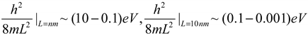 where , is the mass of an electron participating in a CDW, and is the size of a pinned CDW. A clue of this resonance mechanism in HTSC is based on the work by Inosov et al. [21], who assigned the spin resonance to some collective mode.
We next consider the magnetic field dependence in normal metallic states [22]. From previous work [23], the relation between magnetic field and temperature is given as:
where is a constant, is the Bohr magneton, and the diagonal and off-diagonal conductivity are:
where and are constants.
Let us consider the superconducting condensations.
The relation between BCS condensation and Bose-Einstein condensation has been long-standing controversial. Here we suggest a counterproposal as capacitive condensation.
We call a resistance (R) and a capacitance (C) and a voltage (V) in a circuit as RC.
Under the postulation that a Cooper pair have (R,-R), two RC circuits happen as (R, C1,V),
(-R, -C2,-V) and capacitive condensation may occur. The negative resistance for a Cooper pair will be discussed in a later work. In brief, in the process of phonon-mediated interactions between the ion and two electrons, the positive resistance is from same amount of energy loss but the negative resistance may stem from the same amount of energy gain. Let us estimate the negative resistance roughly.
For a Cooper pair, it is given as
and a negative resistance must be induced to conserve zero total momentum.
Finally, under the postulation of zero Coulomb repulsion at pure BCS-type superconducting states, superconducting gap is modified as
Let us consider the experimental clues for our models.
The simplified dome between transition temperature and hole concentration in high transition temperature superconductors (HTSC) [24] may be approximately fitted by 4th-order function of hole concentration as shown in Figure 7.
Amongst may models explaining HTSC, resonance-enhanced theory [25] by ours is given as
To obtain 4th order function, the so called Berry hole [26] as shown in Figure 7 is inevitable to be introduced and
The anomalies in electronic specific heats in HTSCs [27] using Eq. (28) can be explained as
In heavy fermion superconductors (HFSs) block spins must be included in the distribution [16]. There may be a singlet of two block spins governed by Brillouin distribution in depressed resonance with magnons. Even though He superconductors, conventional belief is based on boson of He but we may elucidate differently BCS Cooper pairs in resonance with phasons of phonons.
Let us consider gap symmetries in the presence of Kwangwoon distributions.
Because of electron-hole configurations like charge density wave (CDW) sytems [25], gap symmetries of HTSC become
where , are Fermi wavevectors along x or y-axis, and are gaps independent of wavevectors. Under consideration into electrons and holes, the resultant gap becomes
ee
Let us consider isotope exponents in HTSCs as
where M is the mass of ion.
Isotope exponents can be explained by our model regardless of 0, negative, positive values as shown in Figure 8. As shown in Figure 9, the relation between the band gap and Coulomb repulsions may be approximated as
Using the similar method of Eq. (30) where an electron is equivalent to Berry electron and hole, the superconducting temperature and pseudogap temperature are given by 4th order dependence of hole doping where experimental data [28] for Y-Ba-Cu-O are compared with ours as shown in Figure 10.
The specific heats of He [31] are given as shown below:
in which phononic and electronic ones are described. When phonons undergo freezing, the equation changes:
in which a Fermi level at which electrons are concentrated exists, and zero-point modes of phonons are assumed to be condensed at a specific level.
Based on our previous work [32], the phase of the spin glass may be considered a paramagnetic ordering between block spins comprised by many random spins with most spins aimed in one specific direction. Assuming that all states are possible and that the state is governed by the Fermi–Dirac distributions in a block spin in helium in the presence of magnetic fields along the z-axis, the mean value of the spin operator is given as shown below:
in which can be easily exchanged with other parameters, that is, for pressure, electric field, is the Lande’s factor for a spin, is the Bohr magneton, and is the magnitude of a spin.
From Equations 36–38, the specific heat for 3He [33], in which electrons form a block-like structure, can be explained as shown in equation 39:
in which is a constant, and phonon-freezing is postulated. From the experiment of specific heat for 3He [34], the parameters are obtained and shown below:
where this is in fitting as shown in Figure 11.
In the case of 4He [34], it was assumed that no phonon freezing occurred, and T3 phonon specific heat is dominant. From the point of view of block spins at specific temperatures, block spins in He I states may be dominant above a specific temperature, however, below this temperature, single spins in He II phases are in the majority. This behavior can be represented in Equation (38) in which the specific heat is given as shown below:
The total specific heat is given as shown below:
From Equation (42), this process in He behaves as a lambda-transition as shown in Figure 12 based on [35].
It can be assumed that the pseudo latent heat may originate from a difference between higher and lower temperature limits (in fact no latent heat has been observed) as described in Equation 43:
The other constant term may originate from Coulomb repulsions of block spins (electrons) from Eq. (38) as
From Equation (38), Equation (45) can be derived as shown below:
for which a temperature-quadratic dependence of Coulomb repulsions can be assumed and is the Lande’s factor for a block spin.
From the original derivation [31], the specific heat of He can be given as shown below:
In some HTSC materials, the resistivity may be dominant and dependent on quadratic temperature [36]. It can be elucidated as
Let us reintroduce heavy fermion superconductors [16].
The distribution termed Brillouin is given as
Using the BCS scheme, the energy gap, from the singlet pairing of block spins with antiparallel spin configuration, may be obtained as
where this singlet block Cooper pair may be in resonance with some mode, i.e.,) magnons.
Here using appropriate values of effective mass and effective charge, , respectively. As shown in Figure 1 in Ref [16], in the presence of electric fields the effective charge of a block spin can be Let us consider the heat capacity in heavy fermion materials such as CeCu2Si2 and UBe13.
The heat capacity is given as
where is the energy and is the Fermi energy and is the density of states at Fermi level.
The heat capacity is rewritten as
where is a specific mean energy and this calculated heat capacity is in good correspondence with experimental data in CeCu2Si2 and UBe13 [16].
Let us consider the native distributions before forming Boltzmann distributions.
For any distribution, and parameter, , the result is given as
in which the limit is restricted as:
From Eq. (21), the modified FD and BE distributions as “Fermi-Dirac-Koo distribution”, 4th distribution, and “Bose-Einstein-Koo distribution”, 5th distribution are given as shown in the following equations:
in which the constants, ( , ) stem from the continuity conditions, and the Matsubara relation [25] is given as:
and is the energy, is the chemical potential, and those are shown in Figure 13.
From Eq. (17), phasons and amplitudons are derivied as
Let us consider magnetic free spins and magnetic domain walls in viewpoint of Neel antiferromagnet with two sublattices. Magnetic free spins as itinerant phasons may be governed by a distribution, 6th distribution called as “JJKim distribution”,
and magnetic domain walls as stationary amplitudons are governed by a distribution, 7th distribution called as “DJKim distribution”,
and magnetic skyrmions as coupled phason-amplitudons are governed by a distribution, 8th distribution called as “SSLee distribution”,
The saturation of resistivity in HTSC [37] by block spins from Eqs. (12) and (38) can be explained by
4. Conclusion
In summary, the emergence of high-temperature superconductivity in cuprates and pnictides may be attributed to an alternative carrier distribution—a novel arrangement within the framework of the BCS scheme. It’s crucial to distinguish between spin gaps and pseudogaps. Spin gaps may arise from the disparity between the gap at lower temperature limits and another gap at higher temperature limits. On the other hand, pseudogaps represent a type of superconducting gap for electrons, while pure superconducting gaps can be viewed as gaps tailored for holes. The resonance between superconducting electrons following a traditional BCS model and independent charge density waves (CDWs) could propel the attainment of high transition temperature superconductivity. Clues supporting this notion may be found in the magnetic resonance modes observed in cuprates [38]. Nematic orders [39] manifest in high-temperature superconductors (HTSCs) and can be elucidated through electron-hole spin density waves (SDWs), where both electron CDWs and hole CDWs coexist. The absence of a pseudogap in n-type materials [40] is primarily attributed not to a new distribution of electrons and holes but rather to a Fermi-Dirac distribution of electrons as described in Equation (11).
In the presence or absence of magnetic fields, nematic phases are observed [41] in HTSC and can be explained as the resonance between ions and the ionic part of a CDW with spacing, 2a (on the contrary, SDW with spacing, 4a, (a:lattice constant)) because CDWs are electron-ion coupled modes. As an analogy, the patterns in HTSC could be considered as rising through resonance liked the striped patterns of rising when bread is baked. From the stripe patterns [42,43,44], electron-hole CDW (e-h CDW) and e-h SDW may have spacings, 4a, 8a. Fermi arcs [45,46] may be assigned to hole Fermi surface (FS) subtracting from electron FS into remnant arcs. In some HTSC materials within specific doping ranges, CDWs were not observed but these can be solved by the existence of block-CDWs where these are comprised by block spins. I may guess block-CDW and pair density wave and charge density fluctuation are categorized as the same kind [47].
Acknowledgments
This work has been funded by a research grant from Kwangwoon University (2023).
References
- J.R. Schrieffer, Theory of Superconductivity, Benjamin, New York, 1964.
- J. Bardeen, L.N. Cooper, J.R. Schrieffer, Phys. Rev. 108 (1957) 1175.
- J.G. Bednorz, K.A. Müller, Z. Phys. B - Condensed Matter 64 (1986) 189.
- R.J. Birgeneau, M.A. Kastner, A. Aharony, Z. Phys. B - Condensed Matter 71 (1988) 57.
- A. Aharony, R.J. Birgeneau, A. Coniglio, M.A. Kastner, H.E. Stanley, Phys. Rev. Lett. 60 (1988) 1330.
- V. Hizhnyakov, E. Sigmund, Physica C 156 (1988) 655.
- G. Seibold, E. Sigmund, V. Hizhnyakov, Phys. Rev. B 48 (1993) 7537.
- P. Monthoux, D. Pines, Phys. Rev. B 47 (1993) 6069.
- P. Monthoux, J. Phys. Chem. Solids 54 (1993) 1093.
- P. Monthoux, D. Pines, Phys. Rev. B 49 (1994) 4261.
- P.W. Anderson, Science 235 (1987) 1196.
- G. Baskaran, Z. Zou, P.W. Anderson, Solid State Commun. 63 (1987) 973.
- B.L. Altshuler, L.B.Ioffe, Solid State Commun. 82 (1992) 253.
- J.R. de Sousa, J.T.M. Pacobahyba, M. Singh, Solid State Commun. 149 (2009) 131.
- J. Bauer, A.C. Hewson, N. Dupuis, Phys. Rev. B 79 (2009) 214518.
- J.H. Koo, Y. Kim, J. Supercond. Novel Magn. 29 (2016) 9.
- J.B. Ketterson, S.N Song, Superconductivity, pp. 326-327, (Cambridge University Press, New York, 1999).
- J.W. Jewett, R.A. Serway, Physics for Scientists and Engineers with Modern Physics, 8th ed., (Brooks Cole, Singapore, 2010).
- J.H. Koo, K.-S. Lee, J. Korean Phys. Soc., 76 (2020) 834.
- J.H. Koo, J.Y. Jeong, G. Cho, Solid State Commun. 149 (2009) 142.
- D.S. Inosov, et al., Nat. Phys. 6 (2010) 178.
- N. Singh, Physica C 580 (2021) 1353782.
- J.H. Koo, M.K. Lee, J.H. Kim, D.J. Jin, G. Cho, Solid State Commun. 164 (2013) 47.
- E. Fradkin, et al., Rev. Mod. Phys. 87 (2015) 457.
- J.H. Koo, Eur. Phys. J. Plus 136 (2021) 1020.
- Y. Kim, J.H. Koo, unpublished (2023).
- B. Michon, et al., Nature 567 (2019) 218.
- E. Uykur, et al., Phys. Rev. Lett. 112 (2014) 127003.
- L.P. Gor’kov, V.Z. Kresin, Rev. Mod. Phys. 90 (2018) 011001.
- I. Nekrasov, S. Ovchinnikov, J. Supercond. Novel Magn. 35 (2022) 959.
- C. Kittel, Introduction to Solid State Physics, 5th edition, (John Wiley & Sons, New York, 1976).
- J.H. Koo, Physica B 457 (2015) 54.
- J.C. Wheatley, Rev. Mod. Phys. 47 (1975) 415.
- X. Lin, Ph.D. Thesis, (Penn. State University,2008)(unpublished).
- R.J. Donnelly, Physics Today, 30-36, July (1995).
- T. Sarkar, et al., Phys. Rev. B 98 (2018) 224503.
- D. Bhoi, et al., Supercond. Sci. Technol. 21 (2008) 125021.
- Y. Sidis, et al., Phys. Stat. Sol. (b) 241 (2004) 1204.
- A. Chubukov, P.J. Hirschfeld, Physics Today, June (2015) 46.
- R.L. Greene, et al., Annual Rev. Condens. Matter Phys. 11 (2020) 213.
- J.A.W. Straquadine, et al., Phys. Rev. B 100 (2019) 125147.
- J.M. Tranquada, Adv. in Phys. 69 (2020) 437.
- N.K. Gupta, et al., Phys. Rev. B 108 (2023) L121113.
- K. Willa, et al., Phys. Rev. B 108 (2023) 054504.
- X.-C. Wang, Y. Qi, Phys. Rev. B 107 (2023) 224502.
- F. Restrepo, et al., Phys. Rev. B 107 (2023) 174519.
- R. Arpaia, G. Ghiringhelli, J. Phys. Soc. Jpn. 90 (2021) 111005.
Figure 1.
Electrons occupying the site of deleted holes or the site of a vacancy are differentiated.
Figure 1.
Electrons occupying the site of deleted holes or the site of a vacancy are differentiated.
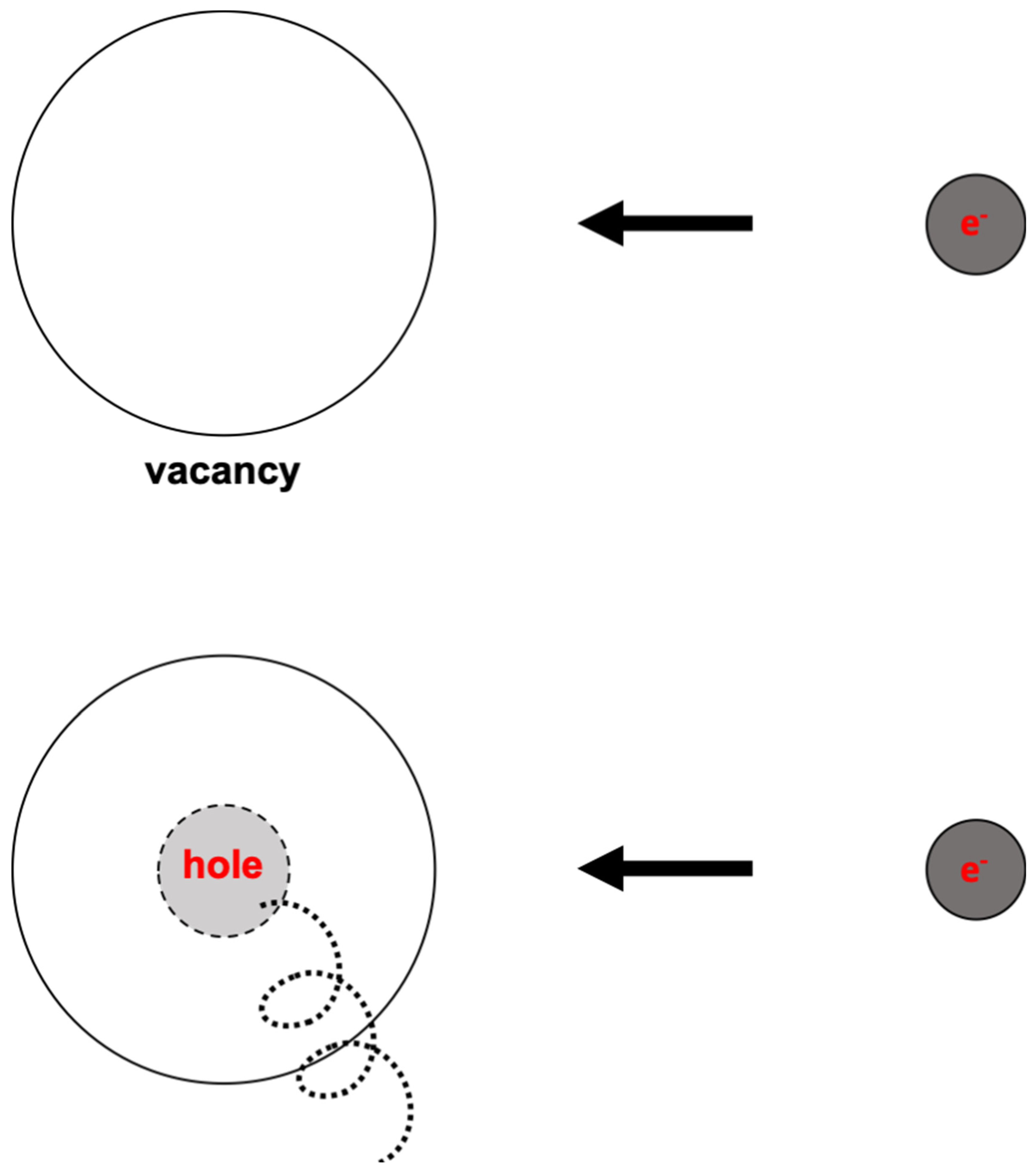
Figure 2.
A spin gap where the Debye cutoff is 150 K.
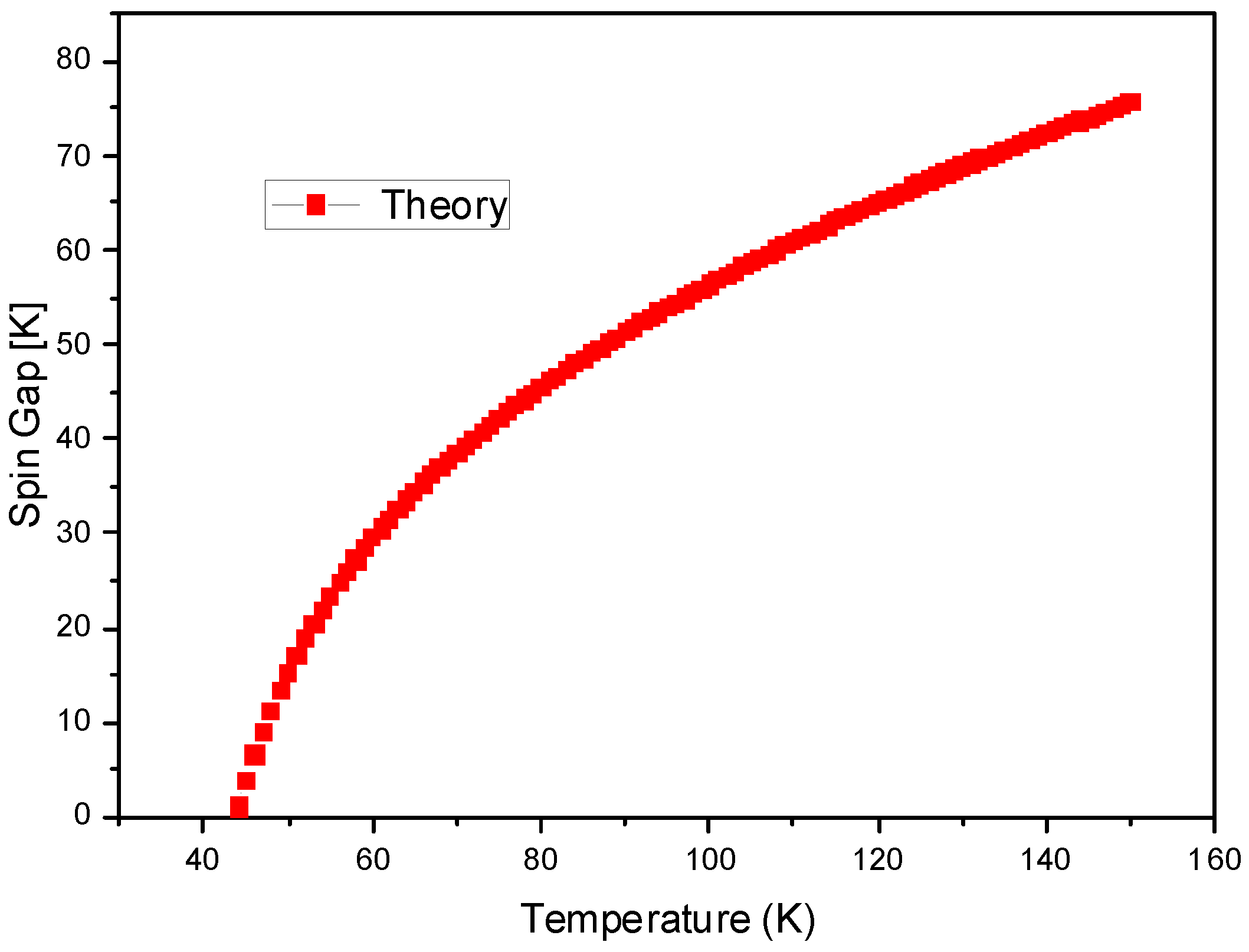
Figure 3.
Natural resonance termed as Josephson resonance between a Cooper pair is shown where the natural thickness of intercalated insulator in a kind of Josephson junction is given to be the resonance energy,
Figure 3.
Natural resonance termed as Josephson resonance between a Cooper pair is shown where the natural thickness of intercalated insulator in a kind of Josephson junction is given to be the resonance energy,
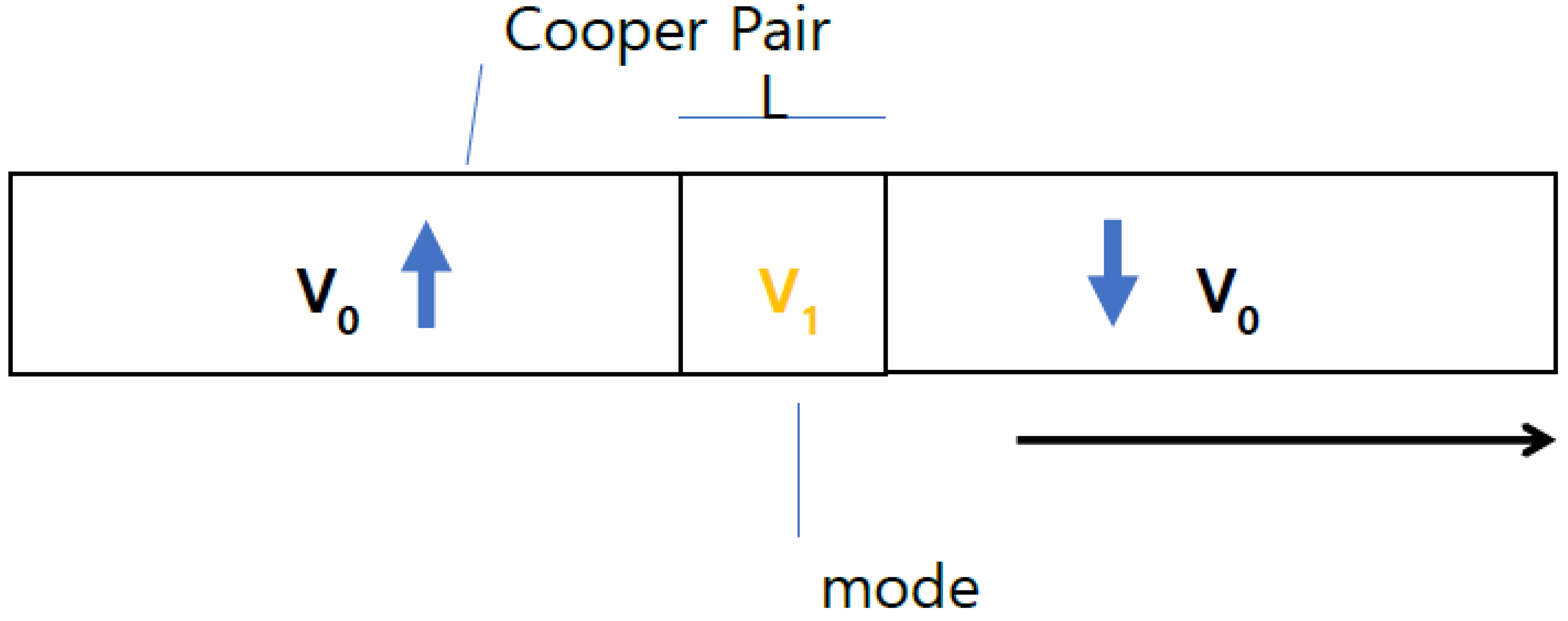
Figure 4.
The superconducting gap is shown where in the presence of Coulomb repulsions it is given by (a) and in the absence of those below 30 K it is also given as (b).
Figure 4.
The superconducting gap is shown where in the presence of Coulomb repulsions it is given by (a) and in the absence of those below 30 K it is also given as (b).
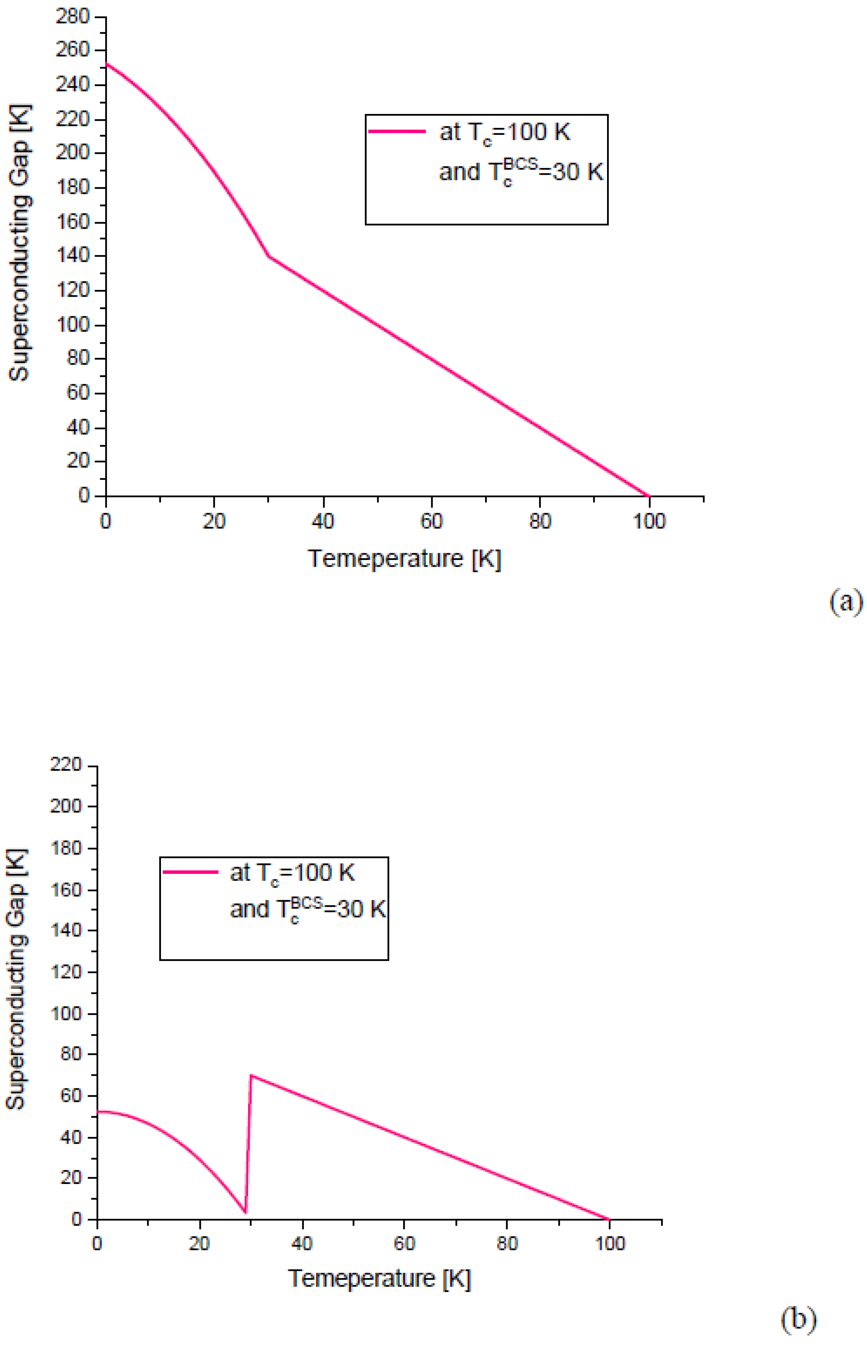
Figure 5.
Calculated (a) and illustrated (b) superconducting gap structures.
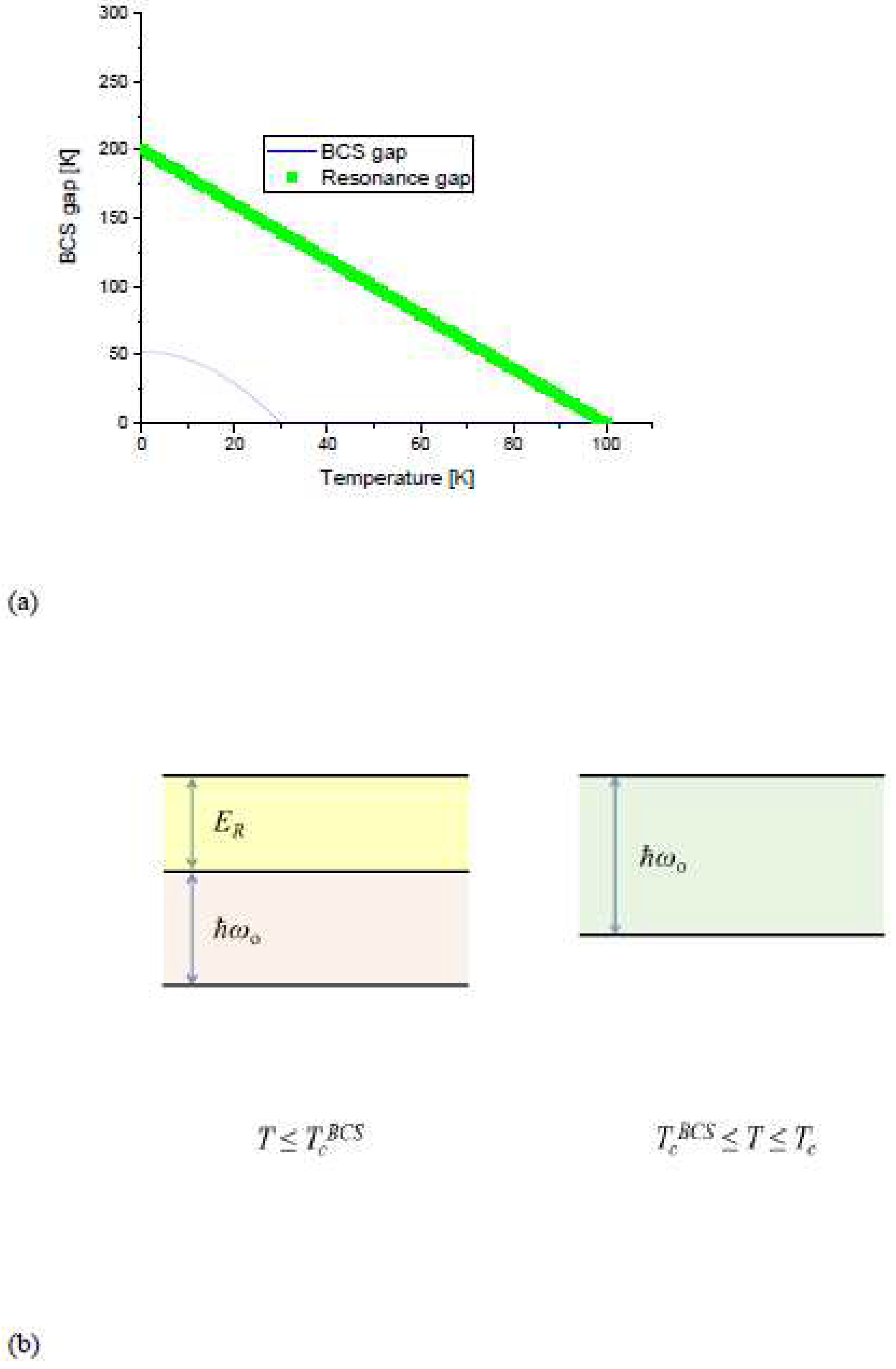
Figure 6.
CDWs confined as (a) energy levels and (b) wavefunctions.
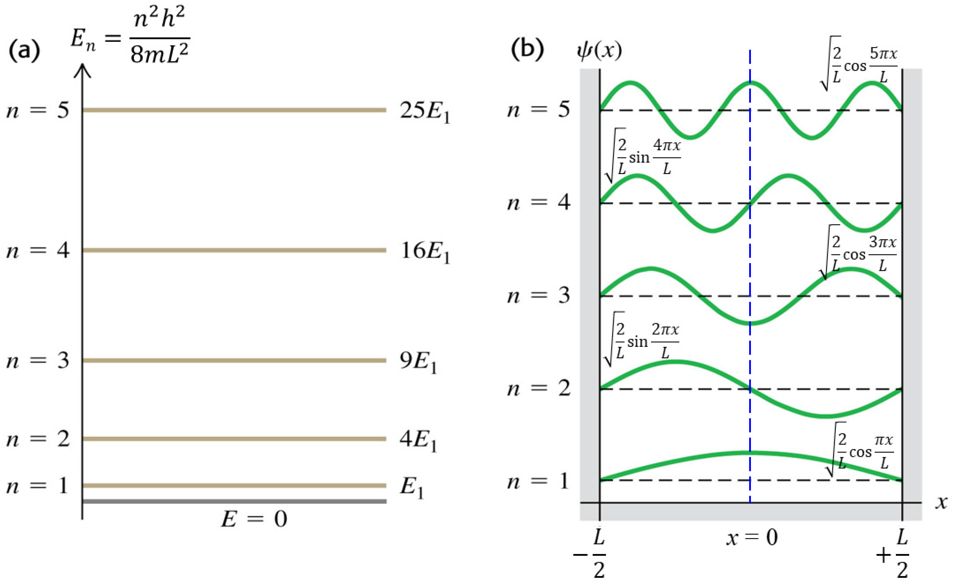
Figure 7.
Simplified dome between transition temperature and hole concentration in high transition temperature superconductors (HTSC) [34] is shown.
Figure 7.
Simplified dome between transition temperature and hole concentration in high transition temperature superconductors (HTSC) [34] is shown.
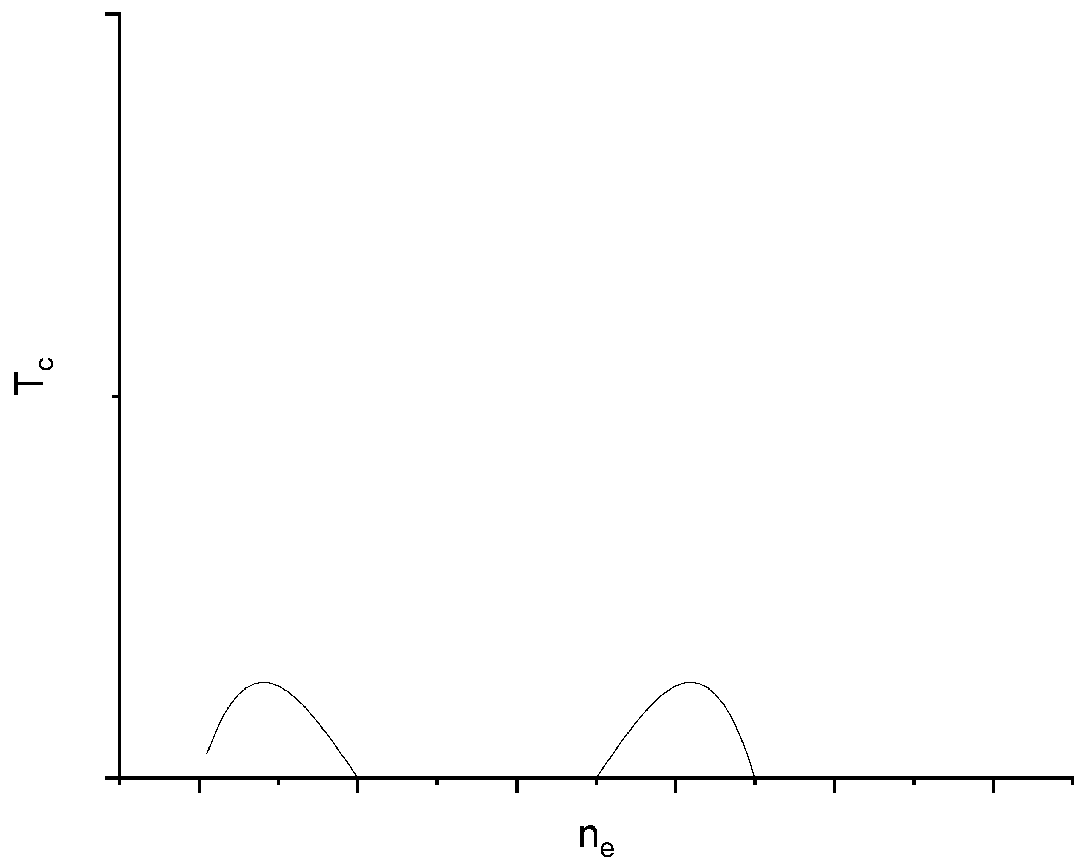
Figure 8.
Isotope exponents are shown.
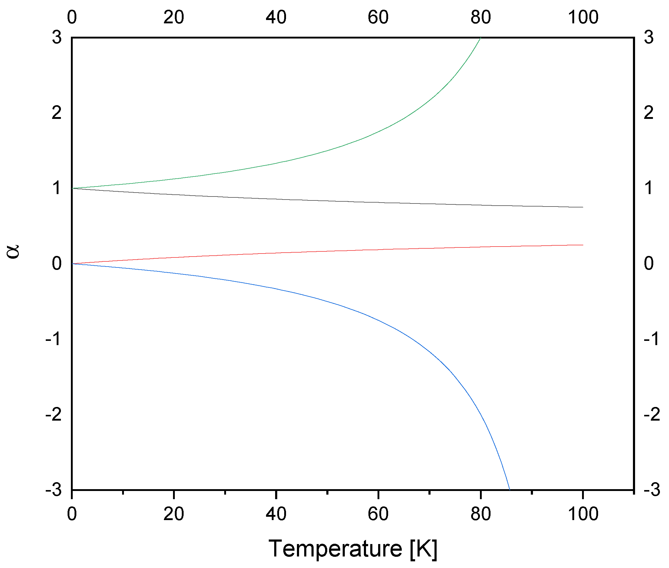
Figure 9.
The phase diagram is shown where Coulomb repulsion between electrons as e-e , e~-e~ may be zero and non-zero for e-e~ and the band gap stems from Coulomb repulsions.
Figure 9.
The phase diagram is shown where Coulomb repulsion between electrons as e-e , e~-e~ may be zero and non-zero for e-e~ and the band gap stems from Coulomb repulsions.
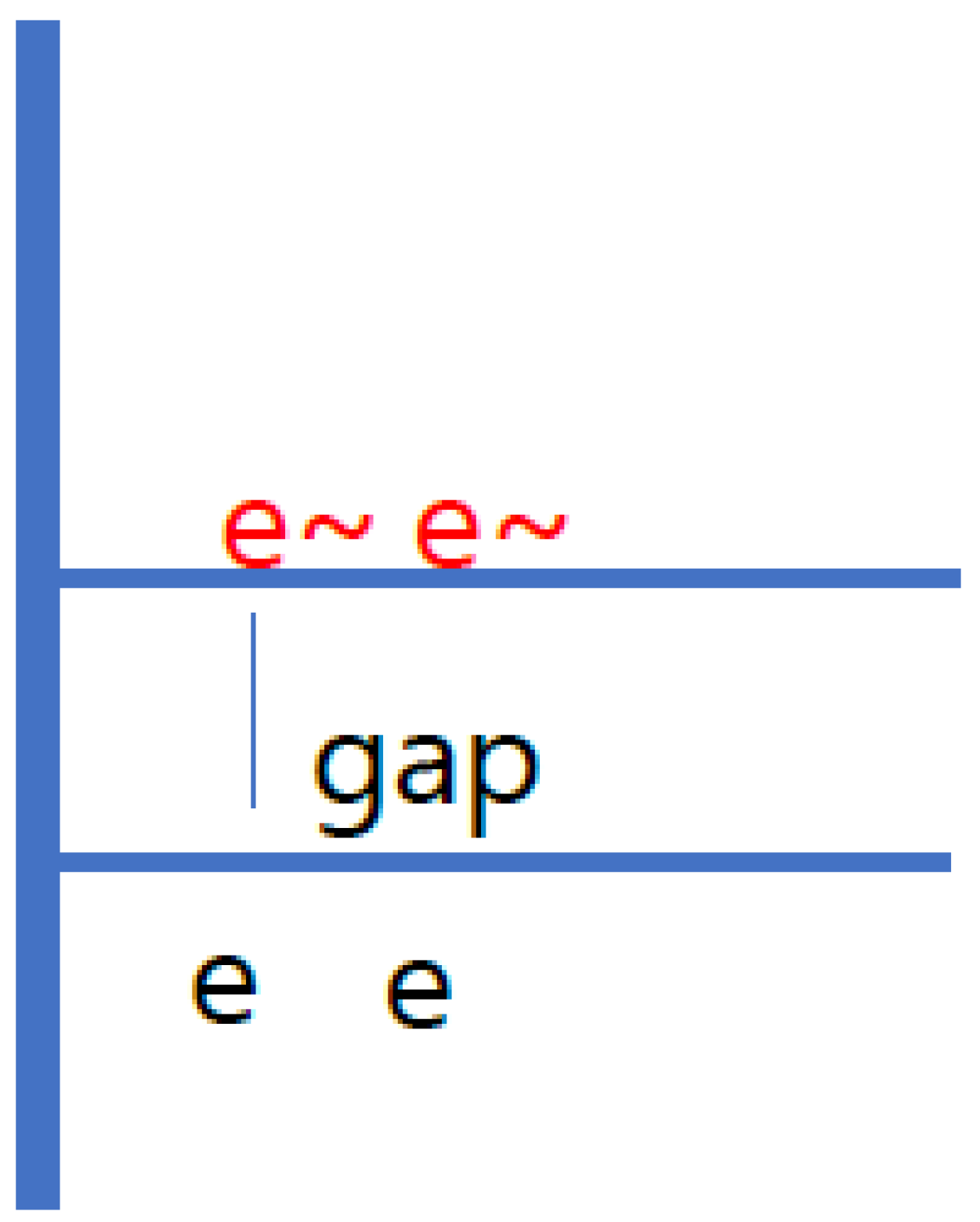
Figure 10.
The phase diagram is shown where fittings are 562.851-23259.3*x+375012*x^2-2.51539*10^6*x^3+6.09134*10^6*x^4 and 2307.53-94601.6*x+1.58875*10^6*x^2-1.16907*10^7*x^3+3.12701*10^7*x^4.
Figure 10.
The phase diagram is shown where fittings are 562.851-23259.3*x+375012*x^2-2.51539*10^6*x^3+6.09134*10^6*x^4 and 2307.53-94601.6*x+1.58875*10^6*x^2-1.16907*10^7*x^3+3.12701*10^7*x^4.
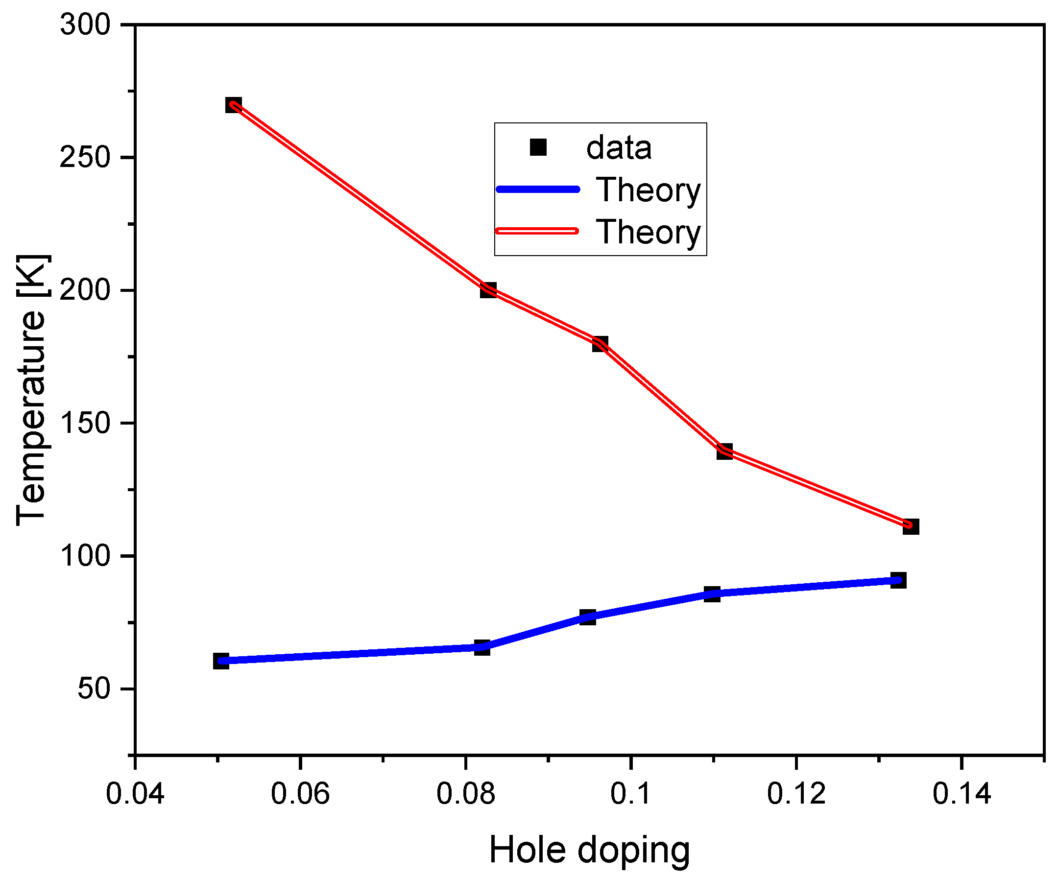
Figure 11.
Heat capacity of 3He is shown.
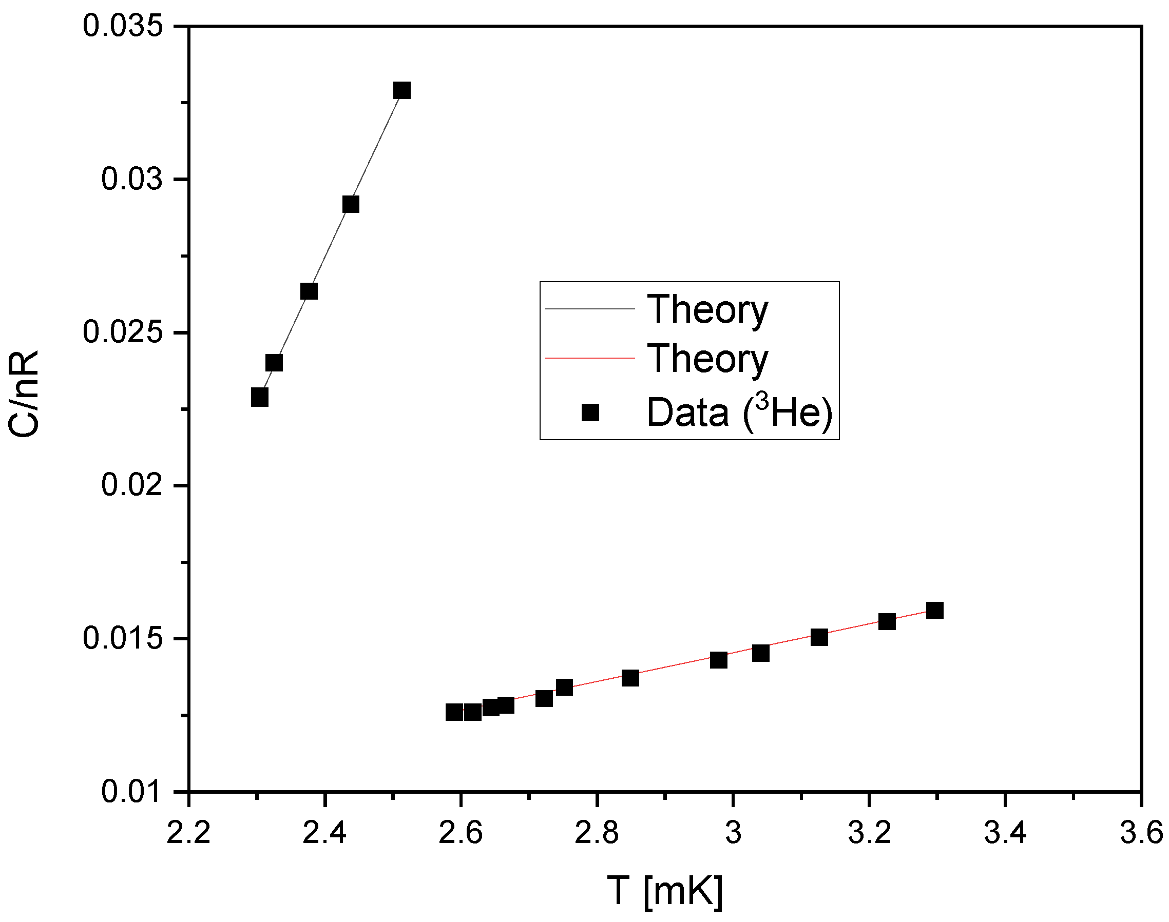
Figure 12.
An arbitrary lambda-transition is roughly shown.
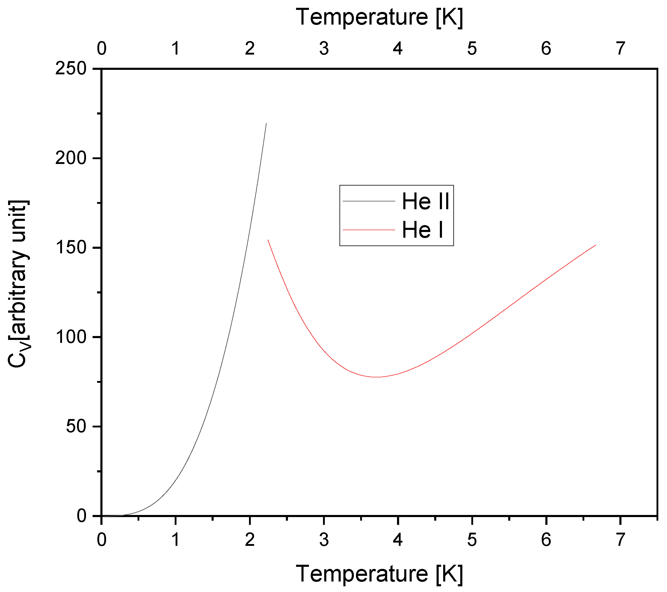
Figure 13.
New distributions are shown for in which the original BE and FD distributions are dominant for .
Figure 13.
New distributions are shown for in which the original BE and FD distributions are dominant for .
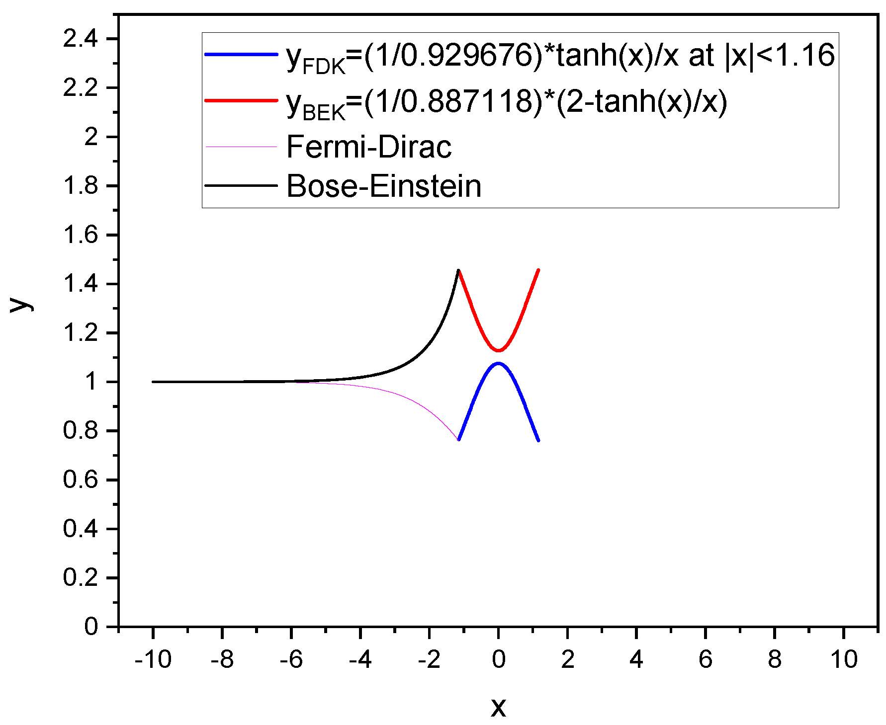

Table 1.
The criteria may be guessed from that in resistivities temperature linear dependences are subject to CDW and flat dependences are subject to magnons.
Table 1.
The criteria may be guessed from that in resistivities temperature linear dependences are subject to CDW and flat dependences are subject to magnons.
| Materials | Resonance with | gain or loss |
| HTSC | Amplitudon of CDW | loss |
| HFS | Phason of magnon | gain |
| Graphene | Phason of phonon | gain |
| He3, He4 | Phason of phonon | gain |
| Organic SC | Phason of CDW | gain or loss |
| Nickelate | Phason of CDW | gain or loss |
| Topological SC | Topological order | gain or loss |
| Ru SC | Phason of Magnon | gain or loss |
| HxS1-x(pressure-induced) | Amplitudon of Magnon | gain or loss |
| Cobalt Oxide SC | Phason of CDW | gain or loss |
Disclaimer/Publisher’s Note: The statements, opinions and data contained in all publications are solely those of the individual author(s) and contributor(s) and not of MDPI and/or the editor(s). MDPI and/or the editor(s) disclaim responsibility for any injury to people or property resulting from any ideas, methods, instructions or products referred to in the content. |
© 2024 by the authors. Licensee MDPI, Basel, Switzerland. This article is an open access article distributed under the terms and conditions of the Creative Commons Attribution (CC BY) license (http://creativecommons.org/licenses/by/4.0/).
Copyright: This open access article is published under a Creative Commons CC BY 4.0 license, which permit the free download, distribution, and reuse, provided that the author and preprint are cited in any reuse.


