
You are currently viewing a beta version of our website. If you spot anything unusual, kindly let us know.
Preprint
Article
Bio–Inspired Space Robotics
Altmetrics
Downloads
135
Views
113
Comments
0
A peer-reviewed article of this preprint also exists.

This version is not peer-reviewed
Abstract
Controlling robots in space with necessarily low material and structural stiffness is quite challenging at least in part due to the resulting very low structural resonant frequencies. The frequencies are sometimes so low, the vary act of controlling the robot with medium or high bandwidth controllers lead to excitation of resonant vibrations. Biomimetics or biomimicry emulates models, systems, and elements of nature for solving such complex problems. Recent seminal publications have re-introduced the viability of optimal command shaping, and one recent instantiation mimics baseball pitching to propose control of highly flexible space robots. The readership will find a perhaps dizzying array of thirteen decently performing alternatives in the literature but could be left bereft selecting a method(s) deemed to be best suited for a particular application. Bio–inspired control of space robotics is presented in a quite substantial (perhaps not comprehensive) comparison, and the conclusions of the study indicate the top three performing methods based on minimizing control effort (i.e., fuel) usage, tracking error mean, and tracking error deviation include.
Keywords:
Subject: Engineering - Mechanical Engineering
1. Introduction
To accumulate energy, baseball pitchers (Figure 1) “wind up”, initially moving the ball in the opposite direction of the desired destination. The general shape of space robots is not dissimilar to baseball pitchers, and this study evaluates the efficacy of trajectory shaping for space robots inspired by the biomimicry of baseball pitching.
1.1. Broad context and why this study is important
Despite recent demonstrations of operations in space of capabilities at the system level of several autonomous functions [5,6] including robotics, contemporary space operations assessment and action planning rely upon pre-scripted sequences of commands from ground operations personnel. [7] Considering challenging and distant robotics missions (e.g., to Mars) ground operators are unlikely to predict all the likely encounters and physical interactions occurring in parts of space seldomly experienced before.[8] Limited knowledge in complex situations demands autonomy, perceivably establishing a new frontier for space exploration. Another obvious example is utilization of very small spacecraft in cislunar orbits to refuel, repair, and replenish earth-orbiting spacecraft at lower altitudes necessitating grappling potentially unknown masses of uncooperative spacecraft. Extreme fuel efficiency seems mandatory, especially due to the low mass and volume of the underactuated robotic repair spacecraft [8] like those depicted in Figure 2, leading naturally to control minimization as a primary figure of merit. [9]
1.1.1. Cislunar space
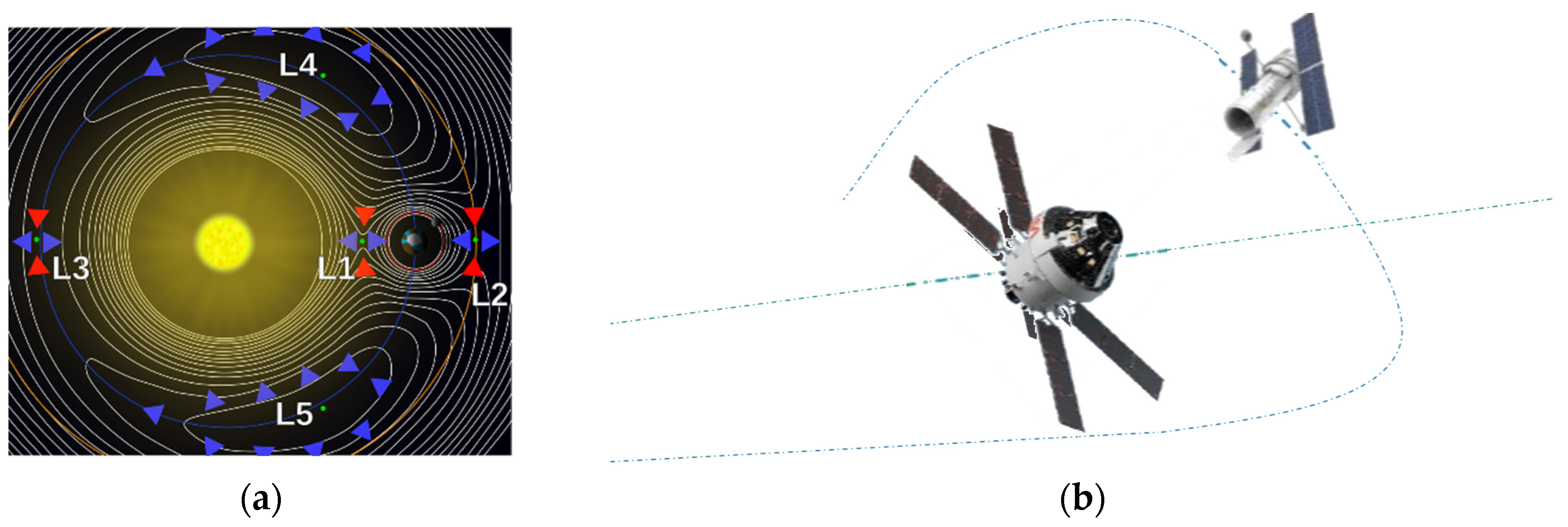
A recent primer on cislunar space published by the U.S. Air Force [13] intended to aid the development of expertise, capabilities, plans, and operational concepts. The importance of the orbits manifested in the December 2019 creation of a new branch of the military charged with the duties to defend and protect American space interests. Especially since highly perturbed orbits depart predictable locations; intercept, rendezvous, and proximity operations (depicted in Figure 3) become quite complicated and potentially unpredictable. Cislunar orbits are generally no longer planar and no longer elliptical (certainly not circular), spacecraft positions are no longer easy to articulate geometrically.
1.1.2. Cislunar robotic operations
Actuators for space robots were recently reviewed in [16] highlighting time–delays as a key limiting issue for successful operations, some of which are displayed in Figure 4. A disparate review [17] assembled (over the last three years), subdivided the trends in research development achievements. The reviews focus on two different treatments of modeling uncertainties in hopes of not needing to increase design margins: either increasing the accuracy of parameter discrimination or alternatively developing methods with inherent robustness. The later review [17] emphasized the fact that task performance execution success correlated with onboard computing power.
In the broadest sense, the space robot (like those depicted in Figure 1, Figure 3, and Figure 5) may be considered generically as a cylindrical main body with a robotic appendage attached, leading to both rigid–body and flexible–body treatments. Figure 5 displays two variations on laboratory hardware replicating space robots. Subfigure (b) is the Navy space robot laboratory hardware that serves as the baseline system analyzed in subsequent sections of this manuscript.

Table 1.
Table of proximal variables and nomenclature 1.
| Variable/acronym | Definition | Variable/acronym | Definition |
| Centerline unit vector | Appendage stiffness | ||
| Control torque | Flexible masses and inertias | ||
| Main body inertia mass moment | Flexible inertia mass moment | ||
| Main body rotation angle | Translation & rotation angles |
1 Such tables are offered throughout the manuscript to aid readability.
The literature reveals many mathematical approaches [13] for modeling and also for control, while the readership might be bereft and confused about which method or combinations of methods should be considered for their particular application. This manuscript compares a recently proposed bio–inspired approach to many of the contemporary alternatives.
1.2. Broad review of modeling and control from first–principles to modern instantiations
Modeling can include external and internal constraints on every particle expressed in a Euclidean space [20], or where Newton’s Laws [21] and Euler’s equation [22], may be combined using Chasle’s theorem [23] to define space robot motion states in six degrees of freedom [24]. Control options include both feedback [25] and feedforward (sometimes necessitating system identification) [26] in addition to shaping of the commanded trajectory to ameliorate the deleterious effects of interactions between the control and robot modes that reduce appendage pointing and positioning accuracy. Feedback control is arguably the best understood to adjust robot performance by designing the closed loop system. [27] Well–established, classical techniques include proportional plus integral plus derivative (PID) control [28] emphasizing oscillation design and maintenance of stability following a commanded movement trajectory. A common modern control method used to minimize a performance measure is the linear quadratic regulator [29] ubiquitously applied to linear time–invariant systems, while the presumption for robotic space missions used for refueling and resupply particularly must assume time-variance, since fuels is being relocated and hardware may be removed and replaced. A less frequently first-used control is feedforward elaborated in [30] to be particularly useful if the movements of the space robot are predictable. Feedforward control is also referred to as open–loop control. The recent resurgence of artificial intelligence has not overlooked space robotics, either particularly for medical purposes. [31,32] Robots can be trained by machine learning algorithms to compensate for varying tasks and environments. The internet of things (IoT) is another newly conceived possibility for robot control remotely and monitoring. [33]
Vibration of flexible bodies is strongly driven by the nature of the (impact) excitation or rate of application of external forces. Accordingly, the dynamics of physical contact is important leading to a field of study known as contact dynamics. Such dynamics are modeled using a so–called Hertz model in reference [34] which studied gripping a non–cooperative spacecraft focusing on contact compliance control. The study highlighted the key nature of vibration of flexible spacecraft parts which could lead to repeated continuous collisions. The high flexibility of the robot arms is a key focus of attention for capturing non–cooperative spacecraft. The study presented simulation experiments indicating compliance control seems key to successful performance.
The natural vibrational frequency of the robotic arms is dominated by the arms’ masses and structural stiffness (resistance to motion, either translational or rotational). Tracking control of variable stiffness actuators was studied in reference [35] highlighting robot arm link motor disturbances and variability in actuator stiffnesses (naturally), which may render tracking control schemes ineffective. A mechanism for learning was proposed to compensate for disturbance uncertainties leading to a novel framework for designing controls starting with back–stepping tuning of feedback control, then parameter tuning with finite switching. Validation was offered using computer simulations.
A well–known method called input shaping from the 1990’s has recently been hybridized in reference [36,37] seeking to address vibration residuals in flexible, multi–mode systems. Modal analysis is used to decouple the system by transforming to the reference frame defined by the modal (eigen) vectors. The command is shaped in the diagonalized modal reference frame, where the three contending alternatives were versine (sinusoidal), ramp, or cycloid plus ramped sinusoidal. The methods were compared in simulation experiments which validated high robustness to parameter uncertainty. The general approach is duplicated in this present manuscript comparing bio–inspired whiplash options.
Reference [38] establishes the present study’s comparative benchmark offered by classical control methods augmented with signal processing filters, and the prequel’s benchmark space robot is the same U.S. Navy system whose natural frequencies of vibration are so low as to be excited by even low–bandwidth feedback systems. The utilization of versine shaping proved superior to step commands when the structural filters were designed to achieve system stability margins (classical gain margin and phase margin). Reference [39] is an intermediate sequel investigation on the same navy space robot system, where so–called systems theory methods of Lev Pontryagin were used to develop an open–loop optimal control to minimize maneuver time with quiescent final conditions. The surprising results indicated a “whiplash” shaped command (initially in a direction opposite the commanded terminal state) minimized maneuver time. Results were produced in a commercial, pseudospectral optimization software, and then validation was performed analytically using six necessary conditions of optimization: (1) Hamiltonian minimization condition; (2) adjoint equations; (3) terminal transversality condition; (4) Hamiltonian final value condition; (5) Hamiltonian evolution equation; and lastly (6) Bellman’s principle. Importantly, the bio-mimicking “whiplash” shaping failed to validate one of the six necessary conditions motivating continuing research (including this present manuscript as a new sequel). The biomimicry whiplash control [39] behavior (depicted earlier in this manuscript in Figure 1) is evaluated in this present study applied to shaping the commanded input rather than as a feedforward control.
In addition to high structural flexibility, motor torque limits and joint flexibility are additional considerations emphasized in reference [40] which presented a model–based autonomous generation method for trajectories assuming base excitation and large time–delays for any communications with earth. Computer simulations for verification were presented alongside validation by laboratory experiments on an air–bearing table.
Operationally, highly flexible space robots need to move around large loads of heavy items potentially leading to large tracking errors. Reference [41] proposed damping–stiffness control including joint dynamics in a comprehensive model utilizing Luenberger observers for unmeasurable quantities. Damping was treated as a feedforward (plus gain), while the feedback is used to suppress perturbations. Verification in simulations hinted at a potential ninety–even percent improvement, while laboratory experiments merely validated an eighty–eight percent improvement.
The dynamics (mathematical models) were the focus of reference [42] seeking the proper element number for inclusion in appendage models, where the end effector trajectory was controlled in the feedforward. Sliding mode control including gravity effects was proposed in reference [43] including nonlinear dynamics typically decomposed into separate flexible and rigid subsystems (as was done in the present manuscript’s study), but modelling accuracy strongly drove performance. As the control of highly flexible robotic systems becomes more commonplace, a MATLAB ®/Simulink® toolbox evolved and was presented in reference [44], effectively reducing the coding burden of future investigations.
1.3. The current state of the research field and key references
Reference [34] describes substantial on-going proof-of-concept investigations including space debris removal, life-extension services, on-orbit assembly, and manufacturing, while identifying remaining challenges, particularly simulation of the true six-degrees-of-freedom dynamics of large-scale microgravity operations, especially for robotic systems. The fourth option, so–called “whiplash shaping” is the bio-inspired method of shaping the input commanded trajectories for the space robot.
- Gain stabilization [45]: Tuning of gain to achieve stability of the rigid body mode.
- Classical second-order structural filtering [45]: Second-order filters designed for each chosen resonance and anti-resonance, usually of lowest mode or lowest two modes to ensure stability.
- Rigid body min-fuel input trajectory shaping: Apply control analytically derived from constrained control–minimization boundary value problem solutions.
- Single-frequency trajectory shaping: Fashion commanded trajectory from single sinusoid chosen to avoid mode frequencies of the flexible robot.
- Flatten the curve to improve stability: Use option #2 to compensate for all structural modes seeking to create a magnitude response curve resembling such a curve for a second-order rigid body system (primary motivation remains increased system stability).
- Flatten the curve to improve trajectory tracking: This option is like option #7, except choosing parts of modes (resonance or anti-resonance) to minimize trajectory tracking errors (proposed in this manuscript).
-
Deterministic artificial intelligence: Use physics to define robot self–awareness, while adapting or learning time–varying physical system parameters (e.g., mass, mass moments, stiffness, damping, etc.).
- 9.1
- Self-awareness statements [52]: Use governing equations from physics to exclusively define robot self–awareness, while prescribing necessary trajectories to be tracked (currently only sinusoidal trajectories and control–minimizing trajectories are in the literature).
- 9.2
1.4. Controversial and diverging hypotheses – literature gaps
Two disparate paradigms are evident regarding response magnitude curve shaping: flattening the curve to improve stability [38] versus flattening the curve to improve trajectory tracking (to be addressed in this manuscript).
1.5. Main aim of the work and highlighting of principal conclusions
The goal is to provide the readership an extensive study comparing performances of available options based on multiple figures of merit: necessary fuel expenditure, mean tracking errors, and tracking error deviations.
1.6. Novelties presented
- Commanded trajectory shaping options are compared using control effort and tracking accuracy, and recommendations are offered.
- Feedforward controls are compared using control effort and tracking accuracy, and recommendations are offered.
- Commanded trajectories are compared with filtered feedback and no feedforward using least control effort tracking accuracy, and recommendations are offered.
- Mode 1 filtering options are compared using control effort tracking accuracy, and recommendations are offered.
- Mode 3 filtering options are compared using control effort tracking accuracy, and recommendations are offered.
- Mode 4 filtering options are compared using control effort tracking accuracy, and recommendations are offered.
- Overall recommendations are made for selection of commanded trajectories, feedforward controls, and filtered versus unfiltered feedback.
- The least control effort was achieved with step trajectories, rigid body optimal feedforward control and unfiltered feedback, while recommendations are offered based on tracking accuracy and control effort.
2. Materials and Methods
Section 2.1 introduces modeling of the highly flexible space robot using as a benchmark the free-floating (on an air-bearing) flexible spacecraft simulator at the Naval Postgraduate School depicted in Figure 6, which also depicts system diagrams including both rigid body and flexible robotic appendage. Development of system models (equations) follows next, where the resulting detailed equations are provided in Appendix A. Section 2.2 introduces competing control methodologies and depicts simulation topologies, where detailed simulation codes are provided in Appendix B.
Selectable options include commanded trajectories, feedforward controls, feedback controls, and structural filtering.
2.1. Space robot modeling
The highly flexible space robot laboratory hardware depicted in Figure 6, subfigure (a) is decomposed into a rigid-body base (simulating the near-rigid spacecraft) depicted in subfigure (b) with highly flexible, lightweight robotic appendages modeled using the finite element method in subfigure (c). The first node of the finite element representation is attached to the spacecraft, while flexible elements (mass and stiffnesses) are lumped at subsequent nodes, where Table 2 conveniently defines variables and nomenclature.
Table 2.
Table of proximal variables and nomenclature 1.
| Variable/acronym | Definition | Variable/acronym | Definition |
| Centerline unit vector | Appendage stiffness | ||
| Control torque | Flexible masses and inertias | ||
| Main body inertia mass moment | Flexible inertia mass moment | ||
| Main body rotation angle | Translation & rotation angles |
1 Such tables are offered throughout the manuscript to aid readability.
Newton’s Law for translational motion is expressed in equation (1) where displacements are expressed in coordinates of an inertial reference frame, while similarly Euler’s moment equations are displayed in equation (2). Expressing motion in coordinates of a non-inertial reference frame modifies equations (1) and (2) to equations (3) and (4) respectively. A representative two-node system of equations including internal flexible “spring forces” that resist motion is displayed in equations (5) and (6) respectively for each node, and then assembled into matrix–vector notation in equation (7), where Table 2 conveniently defines variables and nomenclature.
Table 2.
Table of proximal variables and nomenclature 1
| Variable/acronym | Definition |
| , | Externally applied force & torque expressed in inertial coordinates |
| , | Externally applied force & torque expressed in non-inertial coordinates |
| , | Body’s mass & mass moment of inertia |
| Resulting accelerations expressed in inertial coordinates | |
| , | Angular velocity and acceleration vectors |
| ; | Translational velocity and acceleration vectors |
| Flexible member stiffnesses | |
| Assembled matrices of masses and stiffnesses |
1 Such tables are offered throughout the manuscript to aid readability.
Euler’s moment equations in equation (2) are elaborated for the flexible space robot in equation (8) and resembled in equation (9) to more closely resemble the basic expression of Newton’s Law, where variables and nomenclature are conveniently defined in Table 3.
Isolating the first term of equation (9) leads to equation (10), and slight arithmetic leads to equation (11).
Detailed implementation on the flexible space robot depicted in Figure 6 is included in the appendix to aid repeatability. Mode shapes and (constant) natural vibrational frequencies are obtained by spectral decomposition (i.e. the eigenvalue problem). Meanwhile, mass and moments of inertia (locations of mass) vary leading to time–invariant frequenices and shapes, thus motivating the proposals in this manuscript with the anticipation of future research into deterministic artificial intelligence.
2.2. Competing control design methodologies
Many options are available in the literature to the robot designer to control the highly flexible system in space. The immediate prequels elaborated gain stabilization, classical second-order structural filtering, input-shaping, and whiplash compensation (where whiplash trajectory shaping is implemented in this study). Meanwhile, this present manuscript iterates several remaining trajectory shaping options: rigid body minimum-fuel trajectory shaping, single-frequency sinusoid, and options for flattening the magnitude response plot, while establishing some groundwork to prepare for future efforts with deterministic artificial intelligence.
- Gain stabilization.
- Classical second-order structural filtering.
- Input-shaping
- Whiplash compensation.
- Rigid body minimum-fuel input trajectory shaping.
- Single-frequency trajectory shaping
- Flatten the curve to improve stability.
- Flatten the curve to improve trajectory tracking.
-
Deterministic artificial intelligence
- 9.1
- Self-awareness statements
- 9.2
- Adaption or optimal learning
2.3. Selectable options: Trajectories, feedforward, feedback, and filtering
Figure 7 depicts simulations created in SIMULINK® including subsystems for selectable commanded trajectory, selectable feedforward controls, feedback controller, structural filters, and the selection subsystem to activate feedforward, feedback, and structural filtering. Those subsystems are fed to control the flexible space robot’s subsystem in a unit-feedback loop resulting in a displayable rotation angle.
2.3.1. Commanded trajectories
The Simulink® subsystem used to select between commanded trajectories is displayed in Figure 8(a) including ubiquitous step commands, rigid body control–minimizing optimal commands, whiplash compensation, time–delay input shaped trajectories, and single sinusoidal commanded trajectories. Figure 8(b) displays a subsystem used to formulate trajectories that are non-zero only when maneuvering. Meanwhile Figure 8(c) and Figure 8(d) display notion subsystem outputs.
2.3.2. Feedback filtering
Filtering feedback controls is simulated as depicted in Figure 9(a) where iteration of controls is achieved by a subsystem of manually switches depicted in Figure 9(b). Activation of all structural filtering (four bandpass filters placed at the spectral location of four anti-resonances plus four notch filters placed at the spectral location of four resonance frequencies) results in modifying the frequency response magnitude plot depicted in Figure 10 (a) to Figure 10(b), where the spikes and dips of resonance and anti-resonance respectively have been smoothed by the structural filters. Former analysis designed these filters primarily using stability as motivation, while this present research evaluates several figures of merit including trajectory tracking and control usage. Figure 10(c) and (d) respectively depict notion impacts of notch and bandpass filters on the frequency response magnitude plot (i.e., Bode plot’s magnitude), where Table 4 provides convenient definitions of proximal variables and nomenclature.
2.3.3. Feedforward controls
Feedforward controls are strictly taken as the self-awareness statements in deterministic artificial intelligence, where the intension is to use this manuscript as benchmarks for the seminal development of deterministic artificial intelligence for flexible space robotics in the sequel. For example, presently equation (8) is modified to equation (18) by prescribing the motion states (using the chosen commanded trajectories) and using time-invariant estimates of the physical parameters (e.g., mass, mass moments, stiffnesses, and eventually damping). The sequel will modify equation (9) is modified to equation (19) by prescribing the motion states (using the chosen commanded trajectories) and using time-invariant estimates of the physical parameters (e.g., mass, mass moments, stiffnesses, and eventually damping). develop adaption and learning methods for the estimates making them time-varying. Follow-on work will combine the transport theorem in equation (18) with the rigid–elastic coupled system in equation (19) which should permit deterministic artificial intelligence to learn time-varying natural frequencies stemming from time-varying mass, mass moments, stiffnesses, and damping.
Selectable options for designing commanded trajectories, feedforward and feedback controls, and structural filtering were elaborated in section 2.3. Presently concluding the Methods and Materials, section 3 next presents the parameters used in the simulation experiments, and then presents the results of many experiments.
3. Results
This section provides a concise and precise description of the experimental results favoring multi–plots with accompanying tables of comparative figures of merit to aid the readership’s efforts ascertaining the relative efficacy of the approaches presented. Presented next is the data interpretation, as well as the experimental conclusions that can be drawn, culminating in a very large table of thirteen of the best approaches (of the twenty-six approaches iterated), displayed with comparative figures of merit. Mini summaries are provided allowing the reader to discard thoughts of relatively inferior methods, while continuing to the next set of comparisons, eventually narrowing to a grouping of the best available options of those surveyed. The simulation parameters are provided in Table 5 to aid repeatability of the presented results.
3.1. Comparing commanded trajectories with unfiltered feedback
The first options experiments compared disparate options for comparing commanded trajectories with unfiltered, classical PID feedback control. Space robot rotation angles are displayed versus time (scaled to unity) in Figure 11 with corresponding figures of merit in Table 6 revealing obviously superior tracking performance of using single-sinusoidally shaped commanded trajectories without feedforward control and unfiltered classical PID feedback control. Orders-of-magnitude improvements in trajectory tracking mean error and deviations is achievable with more than three-fold increase in fuel utilization (i.e., control effort).
Interim summary. When comparing commanded trajectories, step trajectories surprisingly led to the least control effort, while single-sinusoid trajectories produce the most accurate tracking with 150% more control effort. Bio–inspired whiplash compensation performed essentially as well as time–delayed input–shaping.
3.2. Comparing feedforward controls with unfiltered feedback
Having compared trajectory shaping options in section 3.1, this section includes the results of direct comparison of disparate options for feedforward control in the presence of unfiltered, classical PID feedback control. Figure 12 reveals relatively superlative performance is obtained by using single-sinusoidally shaped, commanded trajectories with time-delay input-shaped feedforward control in the presence of unfiltered classical feedback controls, where figures of merit in Table 7 reveal the increased trajectory tracking performance necessitates a non-trivial increase in fuel expenditure (control effort).
Interim summary. When comparing feedforward controls, rigid body optimal feedforward with step trajectory command surprisingly led to the least control effort, while time-delay input-shaped feedforward with single-sinusoid trajectories commanded produced the most accurate tracking with 280% more control effort.
3.3. Comparing commanded trajectories with filtered feedback
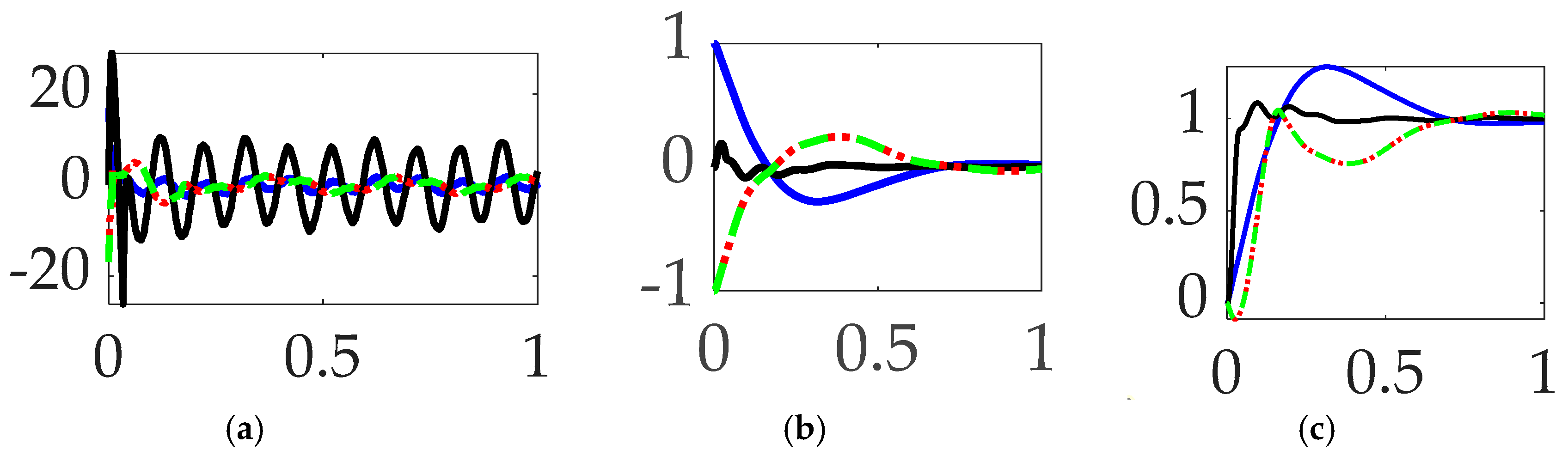
Having discerned the advantages of single-sinusoidally shaped, commanded trajectories and time-delay input-shaped feedforward control, this section repeats the comparison in Section 3.1 (which included only unfiltered feedback), but this time iterates the options when structural filters are use. Figure 13 reveals the lowest control effort (i.e., fuel usage) with nominal tracking performance using unshaped step commands, no feedforward controls with structurally filtered feedback; however, substantially improved target tracking performance is achievable at using higher control efforts by commanding optimal (fuel-minimizing) trajectories that are constrained by rigid-body dynamics equations.
Figure 13.
Selectable commanded trajectory comparative simulation experiments performed in Simulink®. Solid blue line indicates step trajectory, no feedforward, filtered feedback; solid black line indicates rigid body optimal trajectory, no feedforward, filtered feedback; red dotted line indicates whiplash trajectory, no feedforward, filtered feedback; and green dashed line indicates single sine trajectory, no feedforward, filtered feedback (a) control; (b) tracking error, (c) rotation angle. Qualitative results correspond to quantitative figures of merit in Table 8.
Interim summary. When comparing commanded trajectories with filtered feedback and no feedforward, step trajectory commands surprisingly led to the least control effort, while rigid body optimal trajectories achieved an order of magnitude higher accuracy with 2345% more control effort.
3.4. Comparing mode 1 filtering with single-sinusoidal trajectories and no feedforward
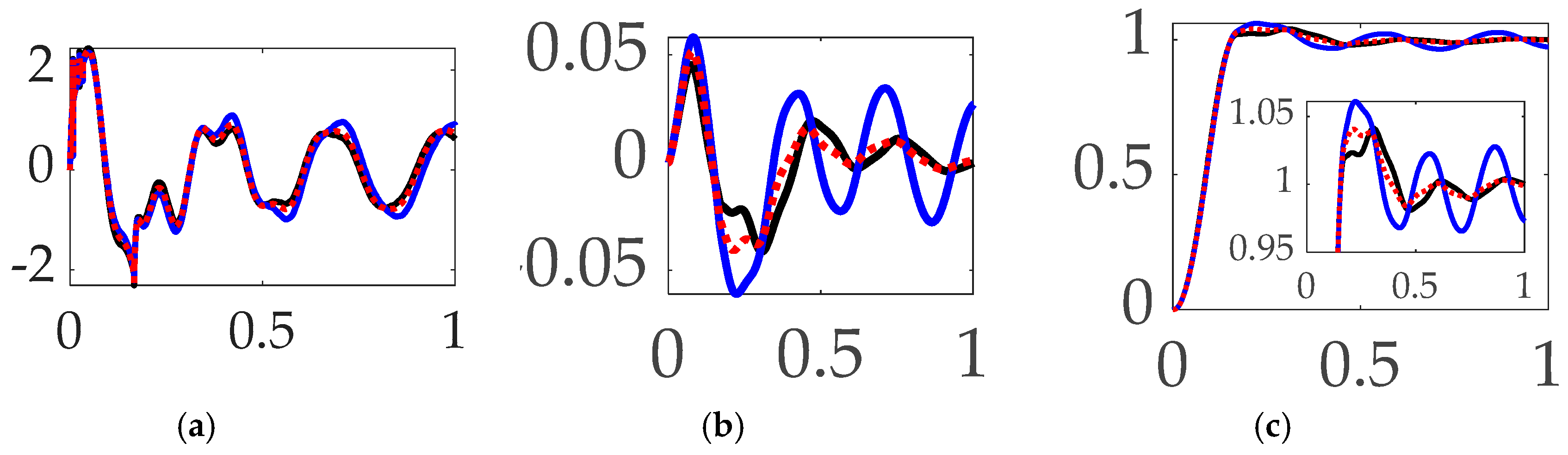
The final sections of the manuscript present experiments with iterated structural filtering: mode 1, mode 2, mode 3, mode 4, and then all of modes 1–4. Single-sinusoidally commanded trajectories are carried over from Section 3.1, Section 3.2 and Section 3.3, identified as a burgeoning best practice. This section iterates compensation of the lowest (first) flexible mode by sequentially compensating for the anti-resonance, the resonance, and then both modal features. The prequel literature predominantly designs structural filters for the sake of stability, often leading to emphasizing notch filtering the first resonant peak, while the results here (designed for target tracking performance rather than stability) indicate superior performance is obtainable by only compensating for the first anti-resonance frequency. This assertion is buttressed by the qualitative results in Figure 13 whose quantitative companion is displayed in Table 9’s display of meaningful performance figures of merit.
Figure 13.
Selectable mode 1 feedback filtering comparative simulation experiments performed in Simulink®. Solid black line indicates single sine trajectory, no feedforward, mode 1 bandpass filtered; solid blue line indicates single sine trajectory, no feedforward, mode 1 notch filtered; red dotted line indicates single sine trajectory, no feedforward, mode 1 bandpass and notch filtered. (a) control; (b) tracking error, (c) rotation angle. Qualitative results correspond to quantitative figures of merit in Table 9.
Interim summary. When comparing mode 1 filtering options bandpass only not-surprisingly led to the least control effort, but surprisingly also produced the most accurate tracking.
3.5. Comparing mode 2 filtering with single-sinusoidal trajectories and no feedforward
Similar to section 3.4’s comparison of the compensation of the first mode, this section sequentially compensates for the second mode’s anti-resonance, resonance, and then both modal components. The results are displayed in Figure 14 which reveal marginal qualitative differences that are validated by quantitative results in Table 10.
Interim summary. When comparing mode 2 filtering options bandpass and notch led to the least control effort, but surprisingly accurate tracking results were inconsistent.
3.6. Comparing mode 3 filtering with single-sinusoidal trajectories and no feedforward
Continuing the evaluation to the third structural mode, like paragraphs 3.4 and 3.5, this paragraph presents the experiment results of sequentially compensating for the third mode’s anti-resonance, resonance, and then both modal components. Similar to the results achieved compensating for the first resonant mode, compensation of the third mode’s bandpass alone proved superior. In this instance, the results are clearly marginal, evidenced in the qualitative displays of Figure 15, where the small differences are quantitatively displayed in Table 11.
Interim summary. When comparing mode 3 filtering options bandpass led to the least control effort and also produced the most accurate tracking accuracy.
3.7. Comparing mode 4 filtering with single-sinusoidal trajectories and no feedforward
The three immediately preceding sections of this manuscript iteratively investigated the first three structural modes, while this paragraph iteratively compensates for the modal components of the fourth structural mode: the anti-resonance, resonance, and then both. Figure 16 (like Figure 15’s qualitative results) reveal marginal results, where inspection of the quantitative results in Table 12 indicate the repeated trend: compensation for the anti-resonance has the largest impact on target tracking errors.
Interim summary. When comparing mode 4 filtering options bandpass led to the least control effort and also produced the most accurate tracking accuracy.
3.8. Comparing modes 1–4 filtering with single-sinusoidal trajectories and no feedforward
Section 3.1, Section 3.2, Section 3.3, Section 3.4, Section 3.5, Section 3.6 and Section 3.7 iteratively examined compensation of individual modal components, while this section simultaneously compensates for all four modes’ anti-resonances followed by all round modes’ resonances. Definite differences are immediately apparent in Figure 17, where the quantitative figures of merit in Table 13 re-validate the discoveries of Section 3.1, Section 3.2, Section 3.3, Section 3.4, Section 3.5, Section 3.6 and Section 3.7: compensation for the anti-resonance alone has the biggest impact on target tracking performance (with a reminder: the opposite result comes from compensating for stability rather than tracking performance).
Interim summary. When comparing modes 1–4 filtering options bandpass not only led to the least control effort but also produced the most accurate tracking accuracy.
3.9. Comparison of the best options studies
This paragraph assembles and compares thirteen common options for controlling highly flexible space robotics providing advice to the readership: should filtered or unfiltered feedback be used? Should feedforward techniques be considered? Is command trajectory shaping effective? From the experiments presented, interesting mixtures of options illustrate efficacy. Table 13 contains a summary of figures of merit achieved by thirteen disparate combinations of available options: input shaping, feedforward and/or feedback control and optional structural filtering.
Interim summary. The least control effort was achieved with step trajectories, rigid body optimal feedforward control and unfiltered feedback, and the effort was 75% less than the average. The best mean tracking error was achieved with sinusoidal trajectories, no feedforward, mode 2 notch filtered, and the tracking error mean was 98% better than the average, while the control effort was 330% higher than the minimum available option. The best tracking error deviation was achieved with sinusoidal trajectories, no feedforward, mode 1–4 bandpass filtered, and the tracking error deviation was 80% better than the average, while the control effort was 42% higher than the minimum available option.
4. Discussion
This section discusses the results and how they can be interpreted from the perspective of previous studies and of the working hypotheses. The findings and their implications are discussed in the broadest context possible. Future research directions are also highlighted. The top seven revelations follow:
- Bio–inspired trajectory shaping (modified from a time–minimization control per [39]) seems confounded in the presence of classical, unfiltered feedback. While the technique performed well, it was not the exemplary option when compared to the multitude of other available options examined.
- When comparing commanded trajectories, step trajectories surprisingly led to the least control effort, while single-sinusoid trajectories produce the most accurate tracking with 150% more control effort. The bio–inspired whiplash shaping was optimized in the cited literature for minimum time in a feedforward control sense, while this sequel reveals the solution is not minimum effort (fuel), nor minimum time in the presence of feedback.
- When comparing feedforward controls, rigid body optimal feedforward with step trajectory command surprisingly led to the least control effort, while time-delay input-shaped feedforward with single-sinusoid trajectories commanded produced the most accurate tracking with 280% more control effort.
- When comparing commanded trajectories with filtered feedback and no feedforward, step trajectory commands surprisingly led to the least control effort, while rigid body optimal trajectories achieved an order of magnitude higher accuracy with 2345% more control effort.
- When comparing mode 1 filtering options bandpass alone not-surprisingly led to the least control effort, but surprisingly also produced the most accurate tracking.
- When comparing mode 3 filtering options bandpass led to the least control effort and also produced the most accurate tracking accuracy.
- When comparing mode 4 filtering options bandpass led to the least control effort and also produced the most accurate tracking accuracy.
- The least control effort was achieved with step trajectories, rigid body optimal feedforward control and unfiltered feedback, and the effort was 75% less than the average. The best mean tracking error was achieved with sinusoidal trajectories, no feedforward, mode 2 notch filtered, and the tracking error mean was 98% better than the average, while the control effort was 330% higher than the minimum available option. The best tracking error deviation was achieved with sinusoidal trajectories, no feedforward, mode 1–4 bandpass filtered, and the tracking error deviation was 80% better than the average, while the control effort was 42% higher than the minimum available option.
4.1. Results in broad context
Reference [38] studied iterations of classical feedback control augmented with structural filters taken from the discipline of signal processing (e.g., notch filters and bandpass filters), where the options were iterated to maximize classical stability margins (i.e., gain margin and phase margin). Alternatively, the feedback–related sections of this investigation iterated the same options towards a goal of minimizing trajectory tracking error.
Meanwhile, reference [39] open loop optimal feedforward was provided for minimizing the maneuver time without the presence of feedback or filtering. The results were bio–inspired, but the time minimizing results did not rank in the top three performances in the present study seeking the best options for target tracking error.
4.2. Controversial or unexpected results
While reference [38] indicates the best selection of options to maximize classical stability margins (i.e., gain margin and phase margin) was attained by only compensating for the first complete flexible mode (resonance and anti-resonance) with notch and bandpass filters, respectively, with step commands shaped by novel single-sinusoidal trajectories.
Meanwhile, the results presented in the present manuscript indicate split results based on lowest control effort, least tracking error mean, or tracking error deviation.
4.2.1. Best control effort
For the best trajectory tracking measured by least control effort, unfiltered feedback (no notch or bandpass filters) is preferred when unshaped step inputs feed rigid body optimal feedforward controls (as displayed in Table 14.
4.2.2. Best tracking error mean
For the best trajectory tracking measured by lowest mean, unfiltered feedback (no notch or bandpass filters) is preferred step inputs and rigid body optimal feedforward controls (as displayed in Table 14.
4.2.3. Best tracking error deviation
For the best trajectory tracking measured by lowest deviation, sinusoidally–shaped commanded trajectories with no feedforward but bandpass–only filtering of modes (as displayed in Table 14.
4.3. Recommended future reseach
A major motivation of the present study is to evaluate the various efficacies of disparate input shaping techniques available to the recently proposed deterministic artificial intelligence method that necessitates such.
4.3.1. Deterministic artificial intelligence
Following the introduction of the feedforward by Cooper/Heidlauf in 2017 [52] applied to chaotic circuits, the seminal introduction of the technique (including both 2–norm optimal feedforward and feedback) was offered by Smeresky/Rizzo [53] applied to spacecraft, despite not yet bearing the name of the technique back in the year 2020. Following the publication of [38,39] comparative prequels, the natural sequels are recommended here as future research: Utilize the trajectories evaluated here for spacecraft as inputs to the deterministic artificial intelligence method to formulate a seminal offering applied to highly flexible space robotics.
Funding
This research received no external funding.
Data Availability Statement
Data supporting reported results can be obtained by contacting the corresponding author.
Conflicts of Interest
The author declares no conflict of interest.
Appendix A. Elaboration of modal system identification on the flexible robot system
Substitute into equation (19):
Recall the expressions for the rigid elastic coupling using modal coordinates: where ’s are mode shapes from finite element analysis using the eigenvalues of K/m (stiffness/mass). The system stiffness matrix is included in Table A1 and mass matrix in Table A2 result in the natural frequencies and mode shapes for the flexible system in Table A3 and Table A4.
Table A1.
Stiffness matrix [K].
| W2 | θ2 | W3 | θ3 | W4 | θ4 | W5 | θ5 | U6 | θ6 | u7 | θ7 | u8 | θ8 | |
| W2 | 958.8179 | 0.0000 | -479.409 | 59.9261 | 0 | 0 | 0 | 0 | 0 | 0 | 0 | 0 | 0 | 0 |
| θ2 | 0.0000 | 19.9754 | -59.9261 | 4.9938 | 0 | 0 | 0 | 0 | 0 | 0 | 0 | 0 | 0 | 0 |
| W3 | -479.409 | -59.926 | 958.8179 | 0.0000 | -479.409 | 59.9261 | 0 | 0 | 0 | 0 | 0 | 0 | 0 | 0 |
| θ3 | 59.9261 | 4.9938 | 0.0000 | 19.9754 | -59.9261 | 4.9938 | 0 | 0 | 0 | 0 | 0 | 0 | 0 | 0 |
| W4 | 0 | 0 | -479.409 | -59.926 | 958.8179 | 0.0000 | -479.409 | 59.9261 | 0 | 0 | 0 | 0 | 0 | 0 |
| θ4 | 0 | 0 | 59.9261 | 4.9938 | 0.0000 | 19.9754 | -59.9261 | 4.9938 | 0 | 0 | 0 | 0 | 0 | 0 |
| W5 | 0 | 0 | 0 | 0 | -479.409 | -59.926 | 479.409 | -59.926 | 0 | 0 | 0 | 0 | 0 | 0 |
| θ5 | 0 | 0 | 0 | 0 | 59.9261 | 4.9938 | -59.9261 | 19.9754 | -59.9261 | 4.9938 | 0 | 0 | 0 | 0 |
| U6 | 0 | 0 | 0 | 0 | 0 | 0 | 0 | -59.926 | 958.8179 | 0.0000 | -479.409 | 59.9261 | 0 | 0 |
| θ6 | 0 | 0 | 0 | 0 | 0 | 0 | 0 | 4.9938 | 0.0000 | 19.9754 | -59.9261 | 4.9938 | 0 | 0 |
| U7 | 0 | 0 | 0 | 0 | 0 | 0 | 0 | 0 | -479.409 | -59.926 | 958.8179 | 0.0000 | -479.409 | 59.9261 |
| θ7 | 0 | 0 | 0 | 0 | 0 | 0 | 0 | 0 | 59.9261 | 4.9938 | 0.0000 | 19.9754 | -59.9261 | 4.9938 |
| U8 | 0 | 0 | 0 | 0 | 0 | 0 | 0 | 0 | 0 | 0 | -479.409 | -59.926 | 479.4089 | -59.926 |
| θ8 | 0 | 0 | 0 | 0 | 0 | 0 | 0 | 0 | 0 | 0 | 59.9261 | 4.9938 | -59.9261 | 9.9877 |
1 Notice state sequence alternates translation, then rotation at each node.
Table A2.
Mass matrix [M]
| Mass | W2 | θ2 | W3 | θ3 | W4 | θ4 | W5 | θ5 | U6 | θ6 | u7 | θ7 | u8 | θ8 |
| W2 | 0.4761 | 0.0000 | 0.0037 | -0.0002 | 0 | 0 | 0 | 0 | 0 | 0 | 0 | 0 | 0 | 0 |
| θ2 | 0.0000 | 0.0000 | 0.0002 | -0.0001 | 0 | 0 | 0 | 0 | 0 | 0 | 0 | 0 | 0 | 0 |
| W3 | 0.0037 | 0.0002 | 4.76E-01 | 0.0000 | 0.0037 | -0.0002 | 0 | 0 | 0 | 0 | 0 | 0 | 0 | 0 |
| θ3 | -0.0002 | -0.0001 | 0.0000 | 0.0000 | 0.0002 | -0.0001 | 0 | 0 | 0 | 0 | 0 | 0 | 0 | 0 |
| W4 | 0 | 0 | 0.0037 | 0.0002 | 0.4761 | 0.0000 | 0.0037 | -0.0002 | 0 | 0 | 0 | 0 | 0 | 0 |
| θ4 | 0 | 0 | -0.0002 | -0.0001 | 0.0000 | 0.0000 | 0.0002 | -0.0001 | 0 | 0 | 0 | 0 | 0 | 0 |
| W5 | 0 | 0 | 0 | 0 | 0.0037 | 0.0002 | 2.63E+00 | -0.0004 | 0 | 0 | 0 | 0 | 0 | 0 |
| θ5 | 0 | 0 | 0 | 0 | -0.0002 | -0.0001 | -0.0004 | 0.0000 | 0.0002 | -0.0001 | 0 | 0 | 0 | 0 |
| U6 | 0 | 0 | 0 | 0 | 0 | 0 | 0 | 0.0002 | 4.76E-01 | 0.0000 | 0.0037 | -0.0002 | 0 | 0 |
| θ6 | 0 | 0 | 0 | 0 | 0 | 0 | 0 | -0.0001 | 0.00E+00 | 0.0000 | 0.0002 | -0.0001 | 0 | 0 |
| U7 | 0 | 0 | 0 | 0 | 0 | 0 | 0 | 0 | 0.0037 | 0.0002 | 0.4761 | 0.0000 | 0.0037 | -0.0002 |
| θ7 | 0 | 0 | 0 | 0 | 0 | 0 | 0 | 0 | -0.0002 | -0.0001 | 0.0000 | 0.0000 | 0.0002 | -0.0001 |
| U8 | 0 | 0 | 0 | 0 | 0 | 0 | 0 | 0 | 0 | 0 | 0.0037 | 0.0002 | 4.66E-01 | -0.0004 |
| θ8 | 0 | 0 | 0 | 0 | 0 | 0 | 0 | 0 | 0 | 0 | -0.0002 | -0.0001 | -0.0004 | 0.0000 |
1 Notice state sequence alternates translation, then rotation at each node.
Table A3.
Natural frequencies, [rad/s]
| 1809.5 | 1415.5 | 1042.2 | 774.3 | 596.8 |
| 478.8 | 410.9 | 54.9 | 43.7 | 30.9 |
| 15.8 | 10.2 | 0.7 | 2.1 |
1 corresponding to mode shapes in Table 5.
Table A4.
Normalized mode shapes [x104]
| -1 | 3 | 2 | 0 | -3 | -5 | 3 | 1501 | 383 | 1037 | 443 | -692 | 181 | 240 |
| -1097 | 3080 | 4481 | 4992 | 4505 | 3173 | -1154 | -4544 | -136 | 2388 | 2221 | 4049 | 1395 | 1669 |
| -1 | 1 | -3 | -7 | -5 | 1 | -2 | -1569 | -215 | 204 | 667 | 1425 | -670 | -712 |
| -2158 | 4857 | 3958 | 28 | -3814 | -4883 | 2208 | -943 | -2040 | -7064 | -867 | 912 | -2460 | -1864 |
| -1 | -1 | -5 | 0 | 7 | 3 | 2 | 1296 | -125 | -1076 | 125 | 995 | -1385 | -1057 |
| -3111 | 4495 | -1058 | -4992 | -1185 | 4481 | -3142 | 5806 | 2118 | 368 | -2572 | 4061 | -3204 | -683 |
| 0 | 0 | 0 | 1 | 1 | -1 | 1 | -99 | 30 | 113 | -105 | 248 | 2247 | 954 |
| -3902 | 2199 | -4861 | -47 | 4875 | -2071 | 3937 | -4288 | -3426 | 4504 | 1878 | 4753 | -3652 | 1689 |
| 0 | -3 | 4 | 0 | -6 | 6 | 1 | 536 | -918 | 135 | 898 | 754 | -946 | 736 |
| -4493 | -1062 | -3138 | 4985 | -3062 | -1232 | -4519 | 815 | 2292 | -2423 | 3091 | 891 | -3893 | 3998 |
| 0 | 2 | 5 | -7 | 7 | -4 | 0 | -294 | 753 | 446 | 880 | 410 | -1936 | 1905 |
| -4872 | -3903 | 2129 | 75 | -2232 | 3920 | 4832 | -2471 | 3385 | -210 | -3658 | 3392 | -4013 | 5178 |
| -1 | -2 | 2 | -3 | 4 | -5 | -6 | 90 | -261 | 192 | -699 | -732 | -2945 | 3254 |
| -5031 | -5052 | 5012 | -5030 | 5062 | -4984 | -4965 | 3580 | -7823 | 3941 | -7649 | -5153 | -4046 | 5502 |
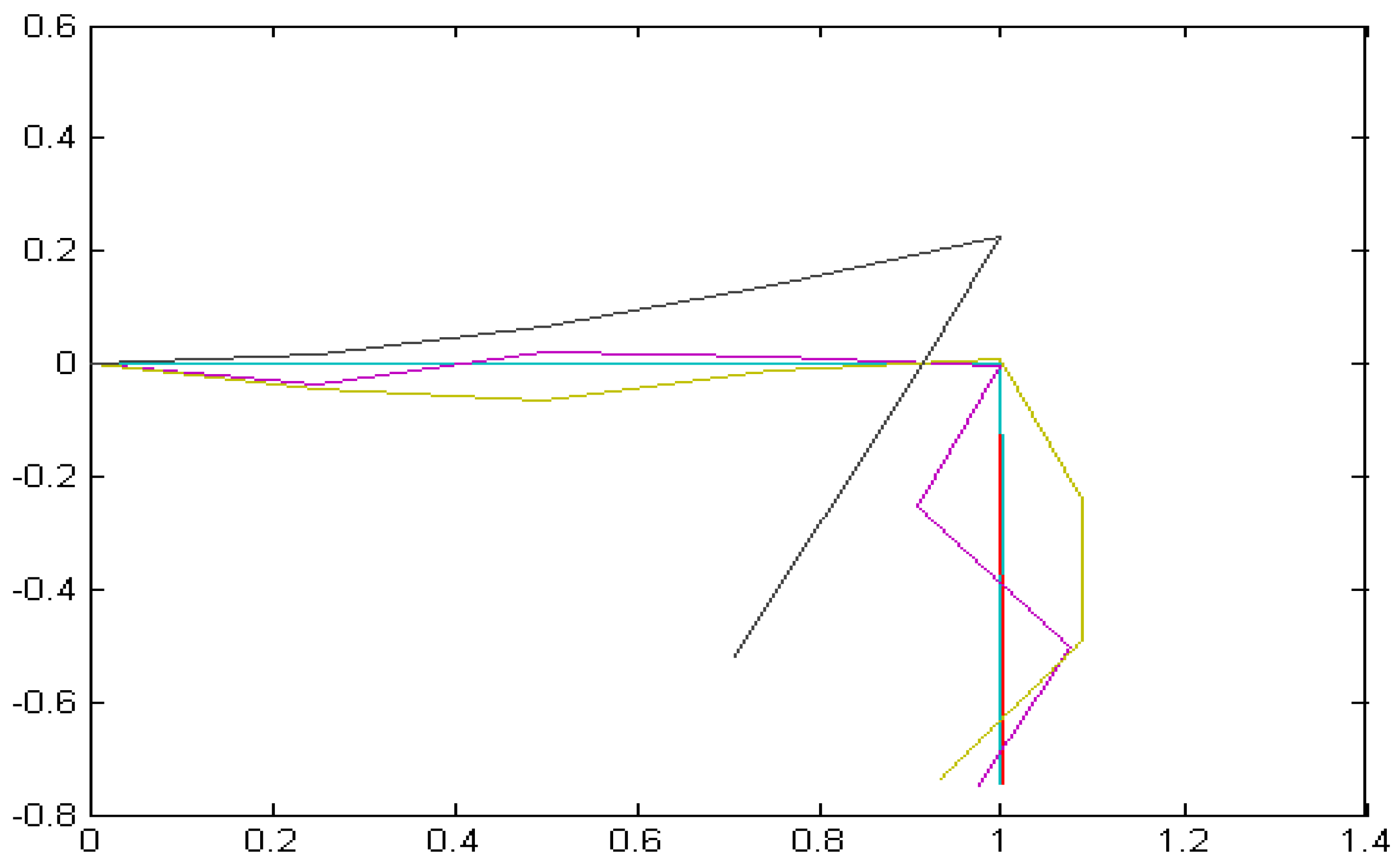
Figure A1.
Normalized mode shapes (modal coordinates) displayed in physical coordinates with normalized length on the abscissa in meters and displacements in meters on the ordinant.
Figure A1.
Normalized mode shapes (modal coordinates) displayed in physical coordinates with normalized length on the abscissa in meters and displacements in meters on the ordinant.
A.1. Equations of Motion in Standard State Space Form
Finite element analysis performed in MATLAB® (code is included in the appendix) generates the mode shapes used to calculate the rigid-elastic coupling terms. The program outputs the flexible system [A], [B], [C], and [D] matrices of the standard state space form. The results are:
Given these equations, the resultant state space matrices are:
Table A5.
State Space [A] matrix.
| 1 | 2 | 3 | 4 | 5 | 6 | 7 | 8 | 9 | 10 | 11 | 12 | |
| 1 | 0 | 0 | 0 | 0 | 0 | 0 | 1 | 0 | 0 | 0 | 0 | 0 |
| 2 | 0 | 0 | 0 | 0 | 0 | 0 | 0 | 1 | 0 | 0 | 0 | 0 |
| 3 | 0 | 0 | 0 | 0 | 0 | 0 | 0 | 0 | 1 | 0 | 0 | 0 |
| 4 | 0 | 0 | 0 | 0 | 0 | 0 | 0 | 0 | 0 | 1 | 0 | 0 |
| 5 | 0 | 0 | 0 | 0 | 0 | 0 | 0 | 0 | 0 | 0 | 1 | 0 |
| 6 | 0 | 0 | 0 | 0 | 0 | 0 | 0 | 0 | 0 | 0 | 0 | 1 |
| 7 | 0 | 0.099 | -1.064 | -3.382 | -0.736 | -26.635 | 0 | 1.392E-04 | -5.066E-04 | -3.298E-04 | -4.662E-05 | -8.609E-04 |
| 8 | 0 | -0.659 | 1.642 | 5.218 | 1.136 | 41.100 | 0 | -9.264E-04 | 7.817E-04 | 5.088E-04 | 7.194E-05 | 1.328E-03 |
| 9 | 0 | 0.188 | -6.435 | -6.433 | -1.401 | -50.670 | 0 | 2.649E-04 | -3.064E-03 | -6.273E-04 | -8.869E-05 | -1.638E-03 |
| 10 | 0 | 0.025 | -0.270 | -106.024 | -0.187 | -6.755 | 0 | 3.531E-05 | -1.285E-04 | -1.034E-02 | -1.182E-05 | -2.183E-04 |
| 11 | 0 | 0.002 | -0.025 | -0.079 | -249.447 | -0.620 | 0 | 3.241E-06 | -1.179E-05 | -7.677E-06 | -1.579E-02 | -2.004E-05 |
| 12 | 0 | 0.022 | -0.233 | -0.742 | -0.162 | -962.998 | 0 | 3.055E-05 | -1.112E-04 | -7.237E-05 | -1.023E-05 | -3.113E-02 |
1 Flexible states where base (rigid body) rotation is controlled.
Appendix B. Initialization Function callbacks for simulation
| clear all; close all; clc; | |||||||
| %This block of code establishes the properties of each beam element a=0.0254; b=0.0016; L=0.25; E=72*10^9; I=a*b^3/12; Li=[12 6*L -12 6*L;6*L 4*L^2 -6*L 2*L^2;-12 -6*L 12 -6*L;6*L 2*L^2 -6*L 4*L^2]; k_beam=E*I/L^3*[Li]; | |||||||
| rho_beam=2.8*10^3; A_beam=a*b; mb=rho_beam*A_beam; |
%Beam density kg/m^3 %Beam cross sectional area %Beam mass per unit length |
||||||
| %This block creates the empty stiffness matrix [k] k=zeros(14,14); | |||||||
| % This block fills in the stiffness matrix components | |||||||
| % Row 1 components start at index=1 k(1,1)=k_beam(3,3)+k_beam(1,1); k(1,2)=k_beam(3,4)+k_beam(1,2); k(1,3)=k_beam(1,3); k(1,4)=k_beam(1,4); |
% Row 2 components start at index=15 k(2,1)=k_beam(4,3)+k_beam(2,1); k(2,2)=k_beam(4,4)+k_beam(2,2); k(2,3)=k_beam(2,3); k(2,4)=k_beam(2,4); |
||||||
| % Row 3 components start at index=29 k(3,1)=k_beam(3,1); k(3,2)=k_beam(3,2); k(3,3)=k_beam(3,3)+k_beam(1,1); k(3,4)=k_beam(3,4)+k_beam(1,2); k(3,5)=k_beam(1,3); k(3,6)=k_beam(1,4); |
% Row 4 components start at index=43 k(4,1)=k_beam(4,1); k(4,2)=k_beam(4,2); k(4,3)=k_beam(4,3)+k_beam(2,1); k(4,4)=k_beam(4,4)+k_beam(2,2); k(4,5)=k_beam(2,3); k(4,6)=k_beam(2,4); |
||||||
| % Row 5 components start at index=59 k(5,3)=k_beam(3,1); k(5,4)=k_beam(3,2); k(5,5)=k_beam(3,3)+k_beam(1,1); k(5,6)=k_beam(3,4)+k_beam(1,2); k(5,7)=k_beam(1,3); k(5,8)=k_beam(1,4); |
% Row 6 components start at index=73 k(6,3)=k_beam(4,1); k(6,4)=k_beam(4,2); k(6,5)=k_beam(4,3)+k_beam(2,1); k(6,6)=k_beam(4,4)+k_beam(2,2); k(6,7)=k_beam(2,3); k(6,8)=k_beam(2,4); |
||||||
| % Row 7 components start at index=89 k(7,5)=k_beam(3,1); k(7,6)=k_beam(3,2); k(7,7)=k_beam(3,3); k(7,8)=k_beam(3,4); |
% Row 8 components start at index=103 k(8,5)=k_beam(4,1); k(8,6)=k_beam(4,2); k(8,7)=k_beam(4,3); k(8,8)=k_beam(4,4)+k_beam(2,2); k(8,9)=k_beam(2,3); k(8,10)=k_beam(2,4); |
||||||
| % Row 9 components start at index=120 k(8,10)=k_beam(2,4); k(9,9)=k_beam(3,3)+k_beam(1,1); k(9,10)=k_beam(3,4)+k_beam(1,2); k(9,11)=k_beam(1,3); k(9,12)=k_beam(1,4); |
% Row 10 components start at index=134 k(10,8)=k_beam(4,2); k(10,9)=k_beam(4,3)+k_beam(2,1); k(10,10)=k_beam(4,4)+k_beam(2,2); k(10,11)=k_beam(2,3); k(10,12)=k_beam(2,4); |
||||||
| % Row 11 components start at index=149 k(11,9)=k_beam(3,1); k(11,10)=k_beam(3,2); k(11,11)=k_beam(3,3)+k_beam(1,1); k(11,12)=k_beam(3,4)+k_beam(1,2); k(11,13)=k_beam(1,3); k(11,14)=k_beam(1,4); |
% Row 12 components start at index=163 k(12,9)=k_beam(4,1); k(12,10)=k_beam(4,2); k(12,11)=k_beam(4,3)+k_beam(2,1); k(12,12)=k_beam(4,4)+k_beam(2,2); k(12,13)=k_beam(2,3); k(12,14)=k_beam(2,4); |
||||||
| % Row 13 components start at index=179 k(13,11)=k_beam(3,1); k(13,12)=k_beam(3,2); k(13,13)=k_beam(3,3); k(13,14)=k_beam(3,4); |
% Row 14 components start at index=193 k(14,11)=k_beam(4,1); k(14,12)=k_beam(4,2); k(14,13)=k_beam(4,3); k(14,14)=k_beam(4,4); |
||||||
| %Display stiffness matrix to check k=k; | |||||||
| %END STIFFNESS MATRIX. START MASS MATRIX | |||||||
| %Assemble individual beam inertia matrix | |||||||
| I_beam=ones(1,8); I_beam=[I_beam.*I]; I_beam(1)=0; |
%Creates empty matrix of I's for eight node points %Fill in matrix values with beam inertia %First node point inertia = 0 |
||||||
| %This block of code creates the individual beam mass matrix "m_beam" mi=[156 22*L 54 -13*L;22*L 4*L^2 13*L -3*L^2;54 13*L 156 -22*L;-13*L -3*L^2 -22*L 4*L^2]; m_beam=mb*L/420*mi; | |||||||
| %This block of code establishes the value of each point mass (mp) %and the system point mass matrix (M) | |||||||
| mp=0.455; | %Point masses, M | ||||||
| M=[0 mp mp mp 2*mp mp mp mp]; | %Matrix of 8 point masses (0 First point mass) | ||||||
| %Creates a 14x14 empty mass matrix [m] m=zeros(14,14); | |||||||
| %Fill in the system mass matrix components | |||||||
| % Row 1 components start at index=1 m(1,1)=m_beam(3,3)+m_beam(1,1)+M(2); m(1,2)=m_beam(3,4)+m_beam(1,2); m(1,3)=m_beam(1,3); m(1,4)=m_beam(1,4); |
% Row 2 components start at index=15 m(2,1)=m_beam(4,3)+m_beam(2,1); m(2,2)=m_beam(4,4)+m_beam(2,2); m(2,3)=m_beam(2,3); m(2,4)=m_beam(2,4); |
||||||
| % Row 3 components start at index=29 m(3,1)=m_beam(3,1); m(3,2)=m_beam(3,2); m(3,3)=m_beam(3,3)+m_beam(1,1)+M(3); m(3,4)=m_beam(3,4)+m_beam(1,2); m(3,5)=m_beam(1,3); m(3,6)=m_beam(1,4) |
% Row 4 components start at index=43 m(4,1)=m_beam(4,1); m(4,2)=m_beam(4,2); m(4,3)=m_beam(4,3)+m_beam(2,1); m(4,4)=m_beam(4,4)+m_beam(2,2); m(4,5)=m_beam(2,3); m(4,6)=m_beam(2,4); |
||||||
| % Row 5 components start at index=59 m(5,3)=m_beam(3,1); m(5,4)=m_beam(3,2); m(5,5)=m_beam(3,3)+m_beam(1,1)+M(4); m(5,6)=m_beam(3,4)+m_beam(1,2); m(5,7)=m_beam(1,3); m(5,8)=m_beam(1,4); |
% Row 6 components start at index=73 m(6,3)=m_beam(4,1); m(6,4)=m_beam(4,2); m(6,5)=m_beam(4,3)+m_beam(2,1); m(6,6)=m_beam(4,4)+m_beam(2,2); m(6,7)=m_beam(2,3); m(6,8)=m_beam(2,4); |
||||||
| % Row 7 components start at index=89 m(7,5)=m_beam(3,1); m(7,6)=m_beam(3,2); m(7,7)=m_beam(3,3)+3*mb+M(5)+M(6)+M(7)+M(8); m(7,8)=m_beam(3,4); | |||||||
| % Row 8 components start at index=103 m(8,5)=m_beam(4,1); m(8,6)=m_beam(4,2); m(8,7)=m_beam(4,3); m(8,8)=m_beam(4,4)+m_beam(2,2); m(8,9)=m_beam(2,3); m(8,10)=m_beam(2,4); |
% Row 9 components start at index=120 m(9,8)=m_beam(3,2); m(9,9)=m_beam(3,3)+m_beam(1,1)+M(6); m(9,10)=m_beam(3,4)+m_beam(1,2); m(9,11)=m_beam(1,3); m(9,12)=m_beam(1,4); |
||||||
| % Row 10 components start at index=134 m(10,8)=m_beam(4,2); m(10,9)=m_beam(4,3)+m_beam(2,1); m(10,10)=m_beam(4,4)+m_beam(2,2); m(10,11)=m_beam(2,3); m(10,12)=m_beam(2,4); |
% Row 11 components start at index=149 m(11,9)=m_beam(3,1); m(11,10)=m_beam(3,2); m(11,11)=m_beam(3,3)+m_beam(1,1)+M(7); m(11,12)=m_beam(3,4)+m_beam(1,2); m(11,13)=m_beam(1,3); m(11,14)=m_beam(1,4); |
||||||
| % Row 12 components start at index=163 m(12,9)=m_beam(4,1); m(12,10)=m_beam(4,2); m(12,11)=m_beam(4,3)+m_beam(2,1); m(12,12)=m_beam(4,4)+m_beam(2,2); m(12,13)=m_beam(2,3); m(12,14)=m_beam(2,4); | |||||||
| % Row 13 components start at index=179 m(13,11)=m_beam(3,1); m(13,12)=m_beam(3,2); m(13,13)=m_beam(3,3)+M(8); m(13,14)=m_beam(3,4); |
% Row 14 components start at index=193 m(14,11)=m_beam(4,1); m(14,12)=m_beam(4,2); m(14,13)=m_beam(4,3); m(14,14)=m_beam(4,4); |
||||||
| %Display the system mass matrix to check m=m; | |||||||
| %Calculate the natural frequencies and normal modes [NormalModes,EigenValues]=eig(inv(m)*k); NaturalFrequencies=diag(EigenValues^0.5); ModeShapes=NormalModes; | |||||||
| %Check Orthogonality like Homework 1 confirm diagonal matrix of 1's %to satisfy equation 24 on slide 17 OrthoMass=NormalModes'*m*NormalModes; OrthoStiff=NormalModes'*k*NormalModes; StiffCheck=OrthoStiff/EigenValues; Equation24_OrthoCheck=diag(diag(StiffCheck/OrthoMass)); | |||||||
| %Spacecraft Radius to be used designating rigid modal coordinate R=0.381; | |||||||
| FeeE=NormalModes; | %Designate Elastic mode shapes array FeeE | ||||||
| Omega=NaturalFrequencies; | %Designate variable name 'Omega' as natural frequencies | ||||||
| %Designate Rigid modal coordinate FeeR FeeR=[R+L 1 R+L*2 1 R+L*3 1 R+L*4 1 -L 1 -L*2 1 -L*3 1]; | |||||||
| Di=FeeE'*m*diag(FeeR); | %Calculate Rigid-Elastic Coupling Coefficient | ||||||
| DiCheck=det(Di); | %Confirm Di is singular...det(Di=0) | ||||||
| Z=0.0005; Izz=14; |
|||||||
| w=diag(NaturalFrequencies); | %Generate a diagonal matrix of natural frequency | ||||||
| Iw=0.0912; | |||||||
| Td=0; Tc=0.1; T=Td+Tc; |
%Disturbance Torque %Control Torque is Iw*qddot_wheel %Total Torque is sum of disturbance and control torques |
||||||
| %Start State Space Development | |||||||
| NatFreq = diag(EigenValues).^0.5; | |||||||
| r = 0.381; | %Radius of the wheel (large rigid body) | ||||||
| freqs = sqrt(EigenValues); % NatFreq = EigenValues(1:5,1:5); freqs = freqs(1:5,1:5); | |||||||
| zeta = 0.0005; | %Given damping ratio for all modes | ||||||
| Izz = 14; | |||||||
| phi_E = NormalModes(1:14,1:5); phi_R = [r+L,1,r+2*L,1,r+3*L,1,r+4*L,1,-L,1,-2*L,1,-3*L,1]'; | |||||||
| M_II = m; Di = [phi_E'*M_II*phi_R]; M_state = [Izz Di'; Di eye(5)]; | |||||||
| C_damp = [zeros(6,6)]; C_damp(2:6,2:6) = 2*zeta*freqs; K=[zeros(6,6)]; K(2:6,2:6) = NatFreq; | |||||||
| A = [zeros(6),eye(6,6); -inv(M_state)*K, -inv(M_state)*C_damp]; Bprime = [1;0;0;0;0;0]; B = [0 0 0 0 0 0 (inv(M_state)*Bprime)']'; C = zeros(12,12); C(1,1)=1; D = zeros(12,1); | |||||||
| [Gnum,Gden] = ss2tf(A,B,C,D); G1 = tf(Gnum(1,:),Gden) | |||||||
| NUM=[1.998e-015 0.1268 0.007582 166.9 5.591 4.718e004 771 3.412e006 1.218e004 1.576e007 1.475e004 7.11e006]; DEN=[1 0.06125 1326 46.15 3.781e005 6683 2.808e007 1.388e005 1.813e008 2.065e005 9.954e007 0 0]; | |||||||
| G=tf(NUM,DEN); | |||||||
| %Put PID controller Transfer function into workspace It=14; Z=0.516931; Bandwidth=4; wn=Bandwidth; T=10/Z/wn; Kd=2*Z*wn*It+It/T; Kp=wn^2+2*Z*wn/T; Ki=wn^2/T; PID=tf([Kd Kp Ki],[0 1 0]); | |||||||
| %DESIGN FILTERS TO SMOOTH OUT MODE 1 %Design Bandpass filter for w = 10^-0.1478 = 0.711541 Hz wz=0.711541;Zz=0.1;wp=wz;Zp=0.0005; BP1=tf([1/wz^2 2*Zz/wz 1],[1/wp^2 2*Zp/wp 1]); PID_BP1=PID*BP1; | |||||||
| %Design Notch filter for w = 10^-0.109 = 0.778037 Hz wz=0.778037;Zz=0.0005;wp=wz;Zp=0.1; Notch1=tf([1/wz^2 2*Zz/wz 1],[1/wp^2 2*Zp/wp 1]); Mode_1=PID*BP1*Notch1; | |||||||
| %DESIGN FILTERS TO SMOOTH OUT MODE 2 %Design Bandpass filter for w = 10^0.3223 wz=10^0.3223;Zz=0.1;wp=wz;Zp=0.0005; BP2=tf([1/wz^2 2*Zz/wz 1],[1/wp^2 2*Zp/wp 1]); | |||||||
| %Design Notch filter for w = 10^0.405 wz=10^0.405;Zz=0.0006;wp=wz;Zp=0.1; Notch2=tf([1/wz^2 2*Zz/wz 1],[1/wp^2 2*Zp/wp 1]); Mode_2=Mode_1*BP2*Notch2; | |||||||
| %Design Lead filter for wz~1, wp~3 %wz=1;Zz=1;wp=3;Zp=1; %Lead=tf([1/wz^2 2*Zz/wz 1],[1/wp^2 2*Zp/wp 1]); %Mode_2=Mode_2*Lead; | |||||||
| %DESIGN FILTERS TO SMOOTH OUT MODE 3 %Design Bandpass filter for w = 10^1.0110 wz=10^1.0110;Zz=0.1;wp=wz;Zp=0.0005; BP3=tf([1/wz^2 2*Zz/wz 1],[1/wp^2 2*Zp/wp 1]); | |||||||
| %Design Notch filter for w = 10^1.0128 wz=10^1.0128;Zz=0.0005;wp=wz;Zp=0.1; Notch3=tf([1/wz^2 2*Zz/wz 1],[1/wp^2 2*Zp/wp 1]); Mode_3=Mode_2*BP3*Notch3; | |||||||
| %DESIGN FILTERS TO SMOOTH OUT MODE 4 %Design Bandpass filter for w = 10^1.49035 wz=10^1.49035;Zz=0.1;wp=wz;Zp=0.0005; BP4=tf([1/wz^2 2*Zz/wz 1],[1/wp^2 2*Zp/wp 1]); | |||||||
| %Design Notch filter for w = 10^1.492 wz=10^1.492;Zz=0.0005;wp=wz;Zp=0.1; Notch4=tf([1/wz^2 2*Zz/wz 1],[1/wp^2 2*Zp/wp 1]); Mode_4=Mode_3*BP4*Notch4; | |||||||
| %CALCULATE SYSTEM NATURAL FREQUENCIES [NaturalFrequencies,Damping,EigenValue]=damp(G); NaturalFrequencies=NaturalFrequencies; | |||||||
Appendix C. Stop Function callbacks for simulation
| [mag1,phase1,wout1] = bode(G); Mag1=20*log10(mag1(:)); Phase1=phase1(:); [mag2,phase2,wout2] = bode(G*PID); Mag2=20*log10(mag2(:)); Phase2=phase2(:); [mag3,phase3,wout3] = bode(G*PID*BP1); Mag3=20*log10(mag3(:)); Phase3=phase3(:); [mag4,phase4,wout4] = bode(G*PID*BP1*Notch1); Mag4=20*log10(mag4(:)); Phase4=phase4(:); [mag5,phase5,wout5] = bode(G*PID*BP1*Notch1*BP2); Mag5=20*log10(mag5(:)); Phase5=phase5(:); [mag6,phase6,wout6] = bode(G*PID*BP1*Notch1*BP2*Notch2); Mag6=20*log10(mag6(:)); Phase6=phase6(:); [mag7,phase7,wout7] = bode(G*PID*BP1*Notch1*BP2*Notch2*BP3); Mag7=20*log10(mag7(:)); Phase7=phase7(:); [mag8,phase8,wout8] = bode(G*PID*BP1*Notch1*BP2*Notch2*BP3*Notch3); Mag8=20*log10(mag8(:)); Phase8=phase8(:); [mag9,phase9,wout9] = bode(G*PID*BP1*Notch1*BP2*Notch2*BP3*Notch3*BP4); Mag9=20*log10(mag9(:)); Phase9=phase9(:); [mag10,phase10,wout10] = bode(G*PID*BP1*Notch1*BP2*Notch2*BP3*Notch3*BP4*Notch4); Mag10=20*log10(mag10(:)); Phase10=phase10(:); figure(1); hold on; semilogx(wout1,Mag1,'--','LineWidth',1); semilogx(wout2,Mag2,'LineWidth',1); semilogx(wout3,Mag3,'--','LineWidth',3); semilogx(wout4,Mag4,':','LineWidth',2); hold off; grid on; axis([0.5,40, -100, 150 ]); set(gca, 'FontSize',28, 'FontName','Palatino Linotype'); legend('Flexible space robot','PID','PID + Bandpass','PID + Notch + Bandpass') figure(2); hold on; set(gca, 'FontSize',28, 'FontName','Palatino Linotype'); semilogx(wout1,Phase1,'--','LineWidth',1); semilogx(wout2,Phase2,'LineWidth',1); semilogx(wout3,Phase3,'--','LineWidth',3); semilogx(wout4,Phase4,':','LineWidth',2); hold off; grid on; figure(3); hold on; semilogx(wout2,Mag2,'--','LineWidth',1); semilogx(wout4,Mag4,'LineWidth',1); semilogx(wout5,Mag5,'--','LineWidth',3); semilogx(wout6,Mag6,':','LineWidth',2); hold off; grid on; axis([0.5,40, -100, 150 ]); set(gca, 'FontSize',28, 'FontName','Palatino Linotype'); legend('PID controlled Flexible space robot','PID+Mode 1','PID + Mode 1 + Bandpass','PID + Mode 1 + Notch + Bandpass') figure(4); hold on; set(gca, 'FontSize',28, 'FontName','Palatino Linotype'); semilogx(wout2,Phase2,'--','LineWidth',1); semilogx(wout4,Phase4,'LineWidth',1); semilogx(wout5,Phase5,'--','LineWidth',3); semilogx(wout6,Phase6,':','LineWidth',2); hold off; grid on; figure(5); hold on; semilogx(wout2,Mag2,'--','LineWidth',1); semilogx(wout4,Mag4,'LineWidth',1); semilogx(wout6,Mag6,'--','LineWidth',3); semilogx(wout7,Mag7,':','LineWidth',2); semilogx(wout8,Mag8,':','LineWidth',2); hold off; grid on; axis([0.5,40, -100, 150 ]); set(gca, 'FontSize',28, 'FontName','Palatino Linotype'); legend('PID controlled Flexible space robot','PID + Mode 1','PID + Mode 2','PID + Mode 1 + Mode 2 + Bandpass','PID + Mode 1 + Mode 2 + Bandpass + Notch') figure(6); hold on; set(gca, 'FontSize',28, 'FontName','Palatino Linotype'); semilogx(wout2,Phase2,'--','LineWidth',1); semilogx(wout4,Phase4,'LineWidth',1); semilogx(wout6,Phase6,'--','LineWidth',3); semilogx(wout7,Phase7,':','LineWidth',2); semilogx(wout8,Phase8,':','LineWidth',2); hold off; grid on; figure(7); hold on; semilogx(wout2,Mag2,'--','LineWidth',1); semilogx(wout4,Mag4,'LineWidth',1); semilogx(wout6,Mag6,'--','LineWidth',3); semilogx(wout8,Mag8,':','LineWidth',2); semilogx(wout9,Mag9,':','LineWidth',2); semilogx(wout10,Mag10,':','LineWidth',2); hold off; grid on; axis([0.5,40, -100, 150 ]); set(gca, 'FontSize',28, 'FontName','Palatino Linotype'); legend('PID controlled Flexible space robot','PID + Mode 1','PID + Mode 2','PID + Mode 1 + Mode 2 + Mode 3','PID + Mode 1 + Mode 2 + Mode 3 + Bandpass + Notch') figure(8); hold on; set(gca, 'FontSize',28, 'FontName','Palatino Linotype'); semilogx(wout2,Phase2,'--','LineWidth',1); semilogx(wout4,Phase4,'LineWidth',1); semilogx(wout6,Phase6,'--','LineWidth',3); semilogx(wout8,Phase8,':','LineWidth',2); semilogx(wout9,Phase9,':','LineWidth',2); semilogx(wout10,Phase10,':','LineWidth',2); hold off; grid on; sys1=G*PID/(1+G*PID); sys2=(G*PID*BP1/(1+G*PID*BP1)); sys3=(G*PID*BP1*Notch1/(1+G*PID*BP1*Notch1)); sys4=(G*PID*BP1*Notch1*BP2/(1+G*PID*BP1*Notch1*BP2)); sys5=(G*PID*BP1*Notch1*BP2*Notch2/(1+G*PID*BP1*Notch1*BP2*Notch2)); sys6=(G*PID*BP1*Notch1*BP2*Notch2*BP3/(1+G*PID*BP1*Notch1*BP2*Notch2*BP3)); sys7=(G*PID*BP1*Notch1*BP2*Notch2*BP3*Notch3/(1+G*PID*BP1*Notch1*BP2*Notch2*BP3*Notch3)); sys8=(G*PID*BP1*Notch1*BP2*Notch2*BP3*Notch3*BP4/(1+G*PID*BP1*Notch1*BP2*Notch2*BP3*Notch3*BP4)); sys9=(G*PID*BP1*Notch1*BP2*Notch2*BP3*Notch3*BP4*Notch4/(1+G*PID*BP1*Notch1*BP2*Notch2*BP3*Notch3*BP4*Notch4)); figure(9); step(sys1,sys2); legend('PID','PID + BP1');set(gca, 'FontSize',28, 'FontName','Palatino Linotype'); figure(10); step(sys1,sys3); legend('PID','PID + BP1+Notch1'); set(gca, 'FontSize',28, 'FontName','Palatino Linotype'); figure(11); step(sys1,sys4); legend('PID','PID + Mode 1 + BP2'); set(gca, 'FontSize',28, 'FontName','Palatino Linotype'); figure(12); step(sys1,sys5); legend('PID','PID + Mode 1 + BP2 + Notch 2'); set(gca, 'FontSize',28, 'FontName','Palatino Linotype'); figure(13); step(sys1,sys6); legend('PID','PID + Mode 1 + Mode 2 + BP3'); set(gca, 'FontSize',28, 'FontName','Palatino Linotype'); figure(14); step(sys1,sys7); legend('PID','PID + Mode 1 + Mode 2 + BP3 + Notch3'); set(gca, 'FontSize',28, 'FontName','Palatino Linotype'); figure(15); step(sys1,sys8); legend('PID','PID + Mode 1 + Mode 2 + Mode 3 + BP4'); set(gca, 'FontSize',28, 'FontName','Palatino Linotype'); figure(16); step(sys1,sys9); legend('PID','PID + Mode 1 + Mode 2 + Mode 3 + BP4 + Notch4'); set(gca, 'FontSize',28, 'FontName','Palatino Linotype'); |
References
- AF, Navy baseball teams square off for 2018 Freedom Classic. Available online: https://www.nellis.af.mil/News/Article/1452330/af-navy-baseball-teams-square-off-for-2018-freedom-classic/ (accessed 12 December 2023).
- Department of Defense Policy. “U.S. Department of Defense photographs and imagery, unless otherwise noted, are in the public domain.” Available online: https://www.defense.gov/Contact/Help-Center/Article/article/2762906/use-of-department-of-defense-imagery (accessed 12 December 2023).
- Nile, R. First Humanoid Robot In Space Receives NASA Government Invention of the Year. Jun 17, 2015. Available online: https://www.nasa.gov/mission_pages/station/research/news/invention_of_the_year (accessed 17 February 2023).
- NASA Image Use Policy. “NASA content (images, videos, audio, etc.) are generally not copyrighted and may be used for educational or informational purposes without needing explicit permissions.” Available online: https://gpm.nasa.gov/image-use-policy (accessed October 8, 2023).
- Nesnas,I.; Fesq, L.; Volpe,R. Autonomy for Space Robots: Past, Present, and Future. Current Robotics Reports 2021, 2, 251–263. [CrossRef]
- Sagan C, Reddy R. Machine intelligence and robotics: report of the NASA Study Group FINAL REPORT. 715-32. 1980. Carnegie Mellon University. Retrieved 2011 7 September. http://www.rr.cs.cmu.edu/NASA%20Sagan%20Report.pdf.
- NASA Autonomous Systems – Systems Capability Leadership Team. Autonomous systems taxonomy. NASA Technical Reports Server. Document ID 20180003082. 2018 14 May. https://ntrs.nasa.gov/citations/20180003082.
- Marshall Spaceflight Center, Advanced Space Transportation Program: Paving the Highway to Space. Available online: https://www.nasa.gov/centers/marshall/news/background/facts/astp.html (accessed on 15 January 2022).
- Curiosity Bot, Advantages and disadvantages of using Robots instead of Astronauts. Available online: https://mycuriositybot.wordpress.com/2019/02/18/advantages–and–disadvantages–of–using–robots–instead–of–astronauts/ (accessed on 18 February 2019).
- NASA is Building a Mission That Will Refuel and Repair Satellites in Orbit. Available online: https://www.universetoday.com/155863/nasa-is-building-a-mission-that-will-refuel-and-repair-satellites-in-orbit/ (accessed October 8, 2023).
- DARPA teams with Northrop Grumman to build robotic service satellites. Available online: https://newatlas.com/space/robotic-service-satellite-darpa-northrop-grumman/ (accessed October 8, 2023).
- Usage Policy. “Images posted on the DARPA website may be used for educational or informational purposes.” Available online: https://www.darpa.mil/policy/usage-policy (accessed October 8, 2023).
- Holzinger, M.; Chow, C.; Garretson, P. A Primer on Cislunar Space, technical report, Air Force Research Labs, May 2021, 7, https://www.afrl.af.mil/Portals/90/Documents/RV/A%20Primer%20on%20Cislunar%20Space_Dist%20A_PA2021-1271.pdf?ver=vs6e0sE4PuJ51QC-15DEfg%3d%3d (accessed October 9, 2023).
- Available online: https://www.ssc.spaceforce.mil/Portals/3/SDA%20Briefings/13.%20Bates_Tyler_SDA%20Industry%20Day_Cislunar%20Space%20SDA_V4.pdf?ver=fhTzhW7RFhI1MDcP90KAuQ%3D%3D (accessed 14 December 2023).
- Image created by NASA used here: https://en.wikipedia.org/wiki/Halo_orbit#/media/File:Lagrange_points2.svg.
- Ellery, A. Tutorial Review on Space Manipulators for Space Debris Mitigation. Robotics 2019, 8(2), 34. [CrossRef]
- Zhang, W.; Li, F.; Li, J.; Cheng, Q. Review of On-Orbit Robotic Arm Active Debris Capture Removal Methods. Aerospace 2023, 10(1), 13. [CrossRef]
- Ai, H.; Zhu, A.; Wang, J.; Yu, X.; Chen, L. Buffer Compliance Control of Space Robots Capturing a Non-Cooperative Spacecraft Based on Reinforcement Learning. Appl. Sci. 2021, 11(13), 5783. [CrossRef]
- Armanini, C; Boyer, F; Mathew, A; Duriez, C; Renda, F. Soft robots modeling: A structured overview. IEEE Transactions on Robotics, Oct. 2022, pp. 1–21. [CrossRef]
- Encyclopaedia Britannica, Britannica, Euclidean space. Available online: https://www.britannica.com/science/Euclidean–space (accessed on 10 October 2022).
- Newton, I. Principia, Jussu Societatis Regiæ ac Typis Joseph Streater; Cambridge University Library: London, UK, 1687.
- Mazalov, V; Parilina, E. The Euler–equation approach in average–oriented opinion dynamics, Mathematics, vol. 8, no. 3, p. 355, 2020. [CrossRef]
- Sands, T. Comparison and Interpretation Methods for Predictive Control of Mechanics. Algorithms 2019, 12(11), 232. [CrossRef]
- A.C.M. Operations, What–are–the–6–degrees–of–freedom, industrial Inspection & Analysis (IIA). Available online: https://industrial–ia.com/what–are–the–6–degrees–of–freedom–6dof–explained/ (accessed on 21 March 2023).
- Doyle, J; Francis, A; Tannenbaum, A. Feedback control theory. Mineola, NY: Dover, 2009.
- Johansson, R; Robertsson, A; Nilsson, K; Verhaegen, M. State–Space System Identification of Robot Manipulator Dynamics. Mechatronics, vol. 10, no. 3, pp 403–418, 2000. [CrossRef]
- Corke, P, “High–performance visual closed–loop robot control,” thesis.
- Li, Y; Ang, K; Chong, G.C.Y., “PID Control System Analysis and design”, IEEE Control Systems, vol. 26, no. 1, pp.32–41, 2006. [CrossRef]
- Bemporad, A; Morari, M; Dua, V; Pistikopoulos, E, “The explicit linear quadratic regulator for constrained systems,” Automatica, vol. 38, no. 1, pp. 3–20, 2002. [CrossRef]
- 30. Tao, K; Kosut, R; Aral, G, “Learning feedforward control,” Proceedings of 1994 American Control Conference –ACC ’94.
- Chang, T; Seufert, C; Eminaga, O; Shkolyar, E, Hu, J; Liao, J, “Current trends in artificial intelligence application for endourology and robotic surgery,” Urologic Clinics of North America, vol 48, no. 1, pp. 151–160. [CrossRef]
- Sands, T. Inducing Performance of Commercial Surgical Robots in Space. Sensors 2023, 23(3), 1510. [CrossRef]
- Fu, S; Bhavsar, P, “Robotic Arm Control based on internet of things,” 2019 IEEE Long Island Systems, Applications and Technology Conference (LISAT), 2019.
- Liu, X.-F.; Zhang, X.-Y.; Cai, G.-P.; Chen, W.-J. Capturing a Space Target Using a Flexible Space Robot. Appl. Sci. 2022, 12(3), 984. [CrossRef]
- Li, J., Ma, K., Wu, Z. Tracking control via switching and learning for a class of uncertain flexible joint robots with variable stiffness actuators. Neurocomputing 2022, 469, 130–137. [CrossRef]
- SEMINAL REFERENCE: INPUT SHAPING .
- Yavuz H.; Mıstıkoğlu, S.; Kapucu, S. Hybrid input shaping to suppress residual vibration of flexible systems. Journal of Vibration and Control 2012, 18(1), 132-140. [CrossRef]
- Sands, T. Flattening the Curve of Flexible Space Robotics. Appl. Sci. 2022, 12(6), 2992. [CrossRef]
- Sands, T. Optimization Provenance of Whiplash Compensation for Flexible Space Robotics. Aerospace 2019, 6(9), 93. [CrossRef]
- Carabis, D.; Wen, J. Trajectory Generation for Flexible-Joint Space Manipulators. Frontiers in Robotics and AI 2022, 9, 687595. [CrossRef]
- Yang, T.; Xu, F.; Zeng, S.; Zhao, S.; Liu, Y.; Wang, Y. A Novel Constant Damping and High Stiffness Control Method for Flexible Space Manipulators Using Luenberger State Observer. Appl. Sci. 2023, 13(13), 7954. [CrossRef]
- Hamad, R. Modelling and Feed-Forward Control of Robot Arms with Flexible Joints and Flexible Links. Master’s Thesis, Chalmers University of Technology, Gothenburg, Sweden, June 2016.
- Li, X.; Yang, D.; Liu, H.. China’s space robotics for on-orbit servicing: the state of the art. National Science Review 2023, 10, 129. [CrossRef]
- Papadopoulos E, Aghili F and Ma O et al. Front Robot AI 2021; 228: 686723.
- Wie, B. Space Vehicle Dynamics and Control. 2nd, American Institute of Aeronautics and Astronautics, Reston, VA, 2008.
- Singhose, W.; Seering, W.; Singer, M. Input Shaping for Vibration Reduction with Specified Insensitivity to Modeling Errors. In Proceedings of Japan-USA Symposium on Flexible Automation, 1. Boston, Massachusetts, USA. July 7-10, 1996.
- Pao, L. Multi-input shaping design for vibration reduction, Automatica 1999 35, 1, 81-89 doi: 10.1016/S0005-1098(98)00124-1. [CrossRef]
- Gorinevsky, D., Vukovich, G.; Nonlinear Input Shaping Control of Flexible Spacecraft Reorientation Maneuver. J. Guid. Con. Dyn 1998 21(2), 264-270. [CrossRef]
- K., Zhengxian, Y. Combined feedback control and input shaping for vibration suppression of flexible spacecraft. In proceedings of the International Conference on Mechatronics and Automation, pp. 3257-3262, Changchun, China. 18 September 2009. https://10.1109/ICMA.2009.5246238.
- Pontryagin, L.; Boltyanskii, V.; Gamkrelidze, R.; Mischenko, E. The Mathematical Theory of Optimal Processes; Neustadt, L.W., Ed.; Wiley: New York, NY, USA, 1962.
- Banginwar, P.; Sands, T. Autonomous Vehicle Control Comparison. Vehicles 2022, 4, 1109–1121. [CrossRef]
- Cooper, M.; Heidlauf, P.; Sands, T. Controlling Chaos—Forced van der Pol Equation. Mathematics 2017, 5(4), 70. [CrossRef]
- Smeresky, B.; Rizzo, A.; Sands, T. Optimal Learning and Self-Awareness Versus PDI. Algorithms 2020, 13(1), 23. [CrossRef]
- Osburn, P.; Whitaker, H.; Kezer, A. New Developments in the Design of Model Reference Adaptive Control Systems. Institute of the Aerospace Sciences papers 1961, 61(39).
- MDPI Image Use Policy. “No special permission is required to reuse all or part of article published by MDPI, including figures and tables. For articles published under an open access Creative Common CC BY license, any part of the article may be reused without permission provided that the original article is clearly cited.” Available online: https://www.mdpi.com/openaccess#:~:text=Permissions-,No%20special%20permission%20is%20required%20to%20reuse%20all%20or%20part,original%20article%20is%20clearly%20cited. (accessed on 14 February 2023).
Figure 1.
Space robots may be represented as cylindrical center rigid bodies and highly flexible appendages. (a) U.S. Naval Academy pitcher throws to home plate at a baseball tournament. (image credit: Technical Sergeant David W. Carbajal) [1,2] (b) NASA’s first humanoid space robot, image credit NASA. [3,4].
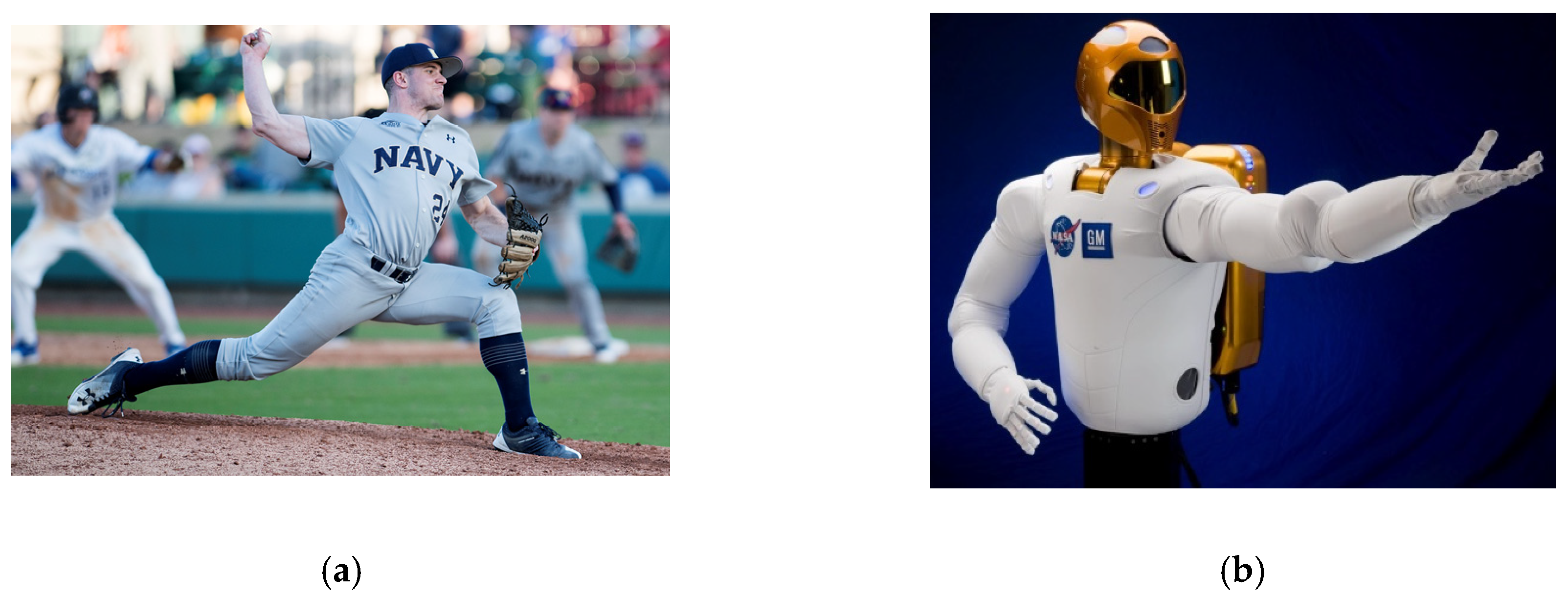
Figure 2.
(a) NASA mission to repair and refuel satellites on–orbit (image credit: NASA [10,4] (b) Satellite servicing mission of the Defense Advanced Research Projects Agency (DARPA). (Image credit: DARPA [11,12].
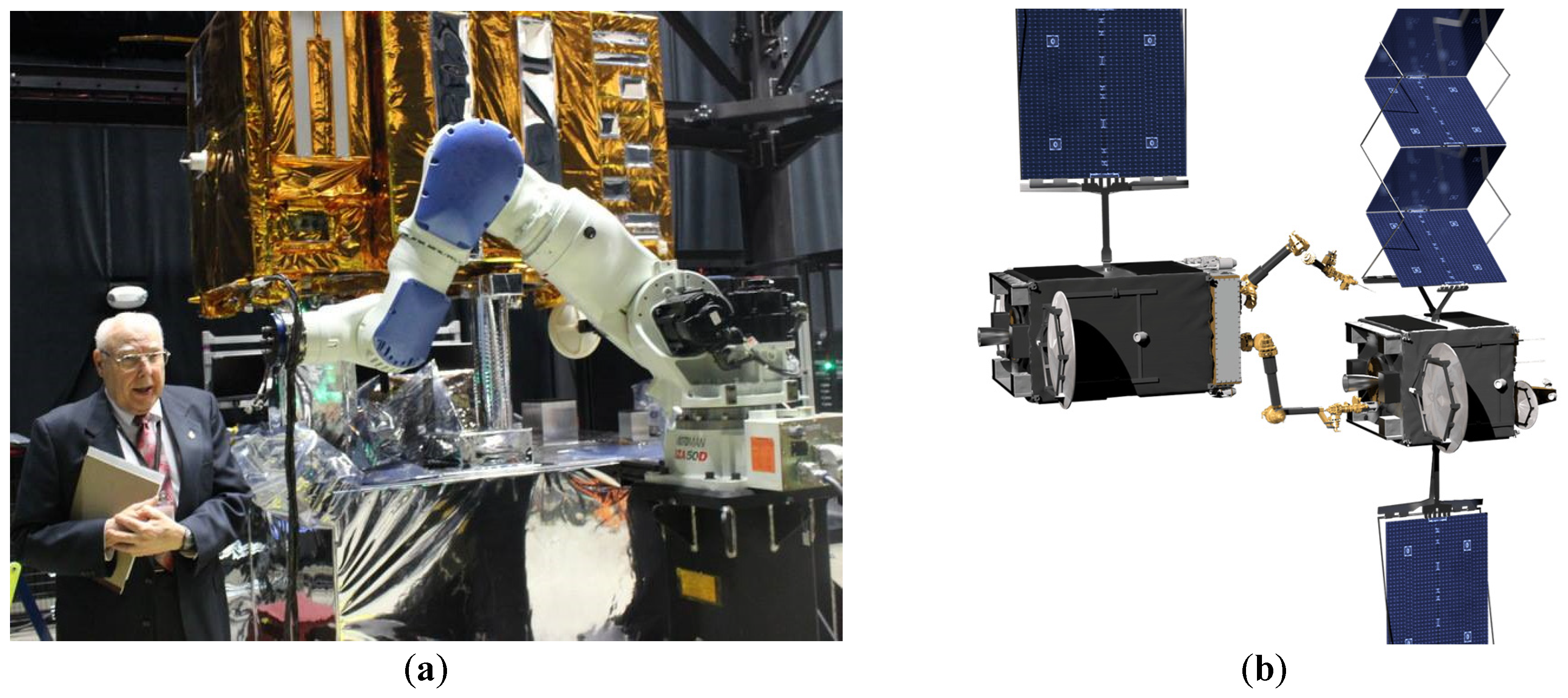
Figure 4.
NASA Robotic Refueling Mission (RRM) task: Refueling. Individual pieces of hardware show the seals that typical satellite fuel valves have. (a) a tertiary cap with "lock wire" visible underneath; (b) a safety cap/actuation nut with securing lock wire. (c) an exposed fuel valve. (d) Safety Cap Tool removing a safety cap; and (e) Nozzle Tool being connected to the now exposed fuel valve enabling fuel transfer. (images credit: NASA [18,4]).
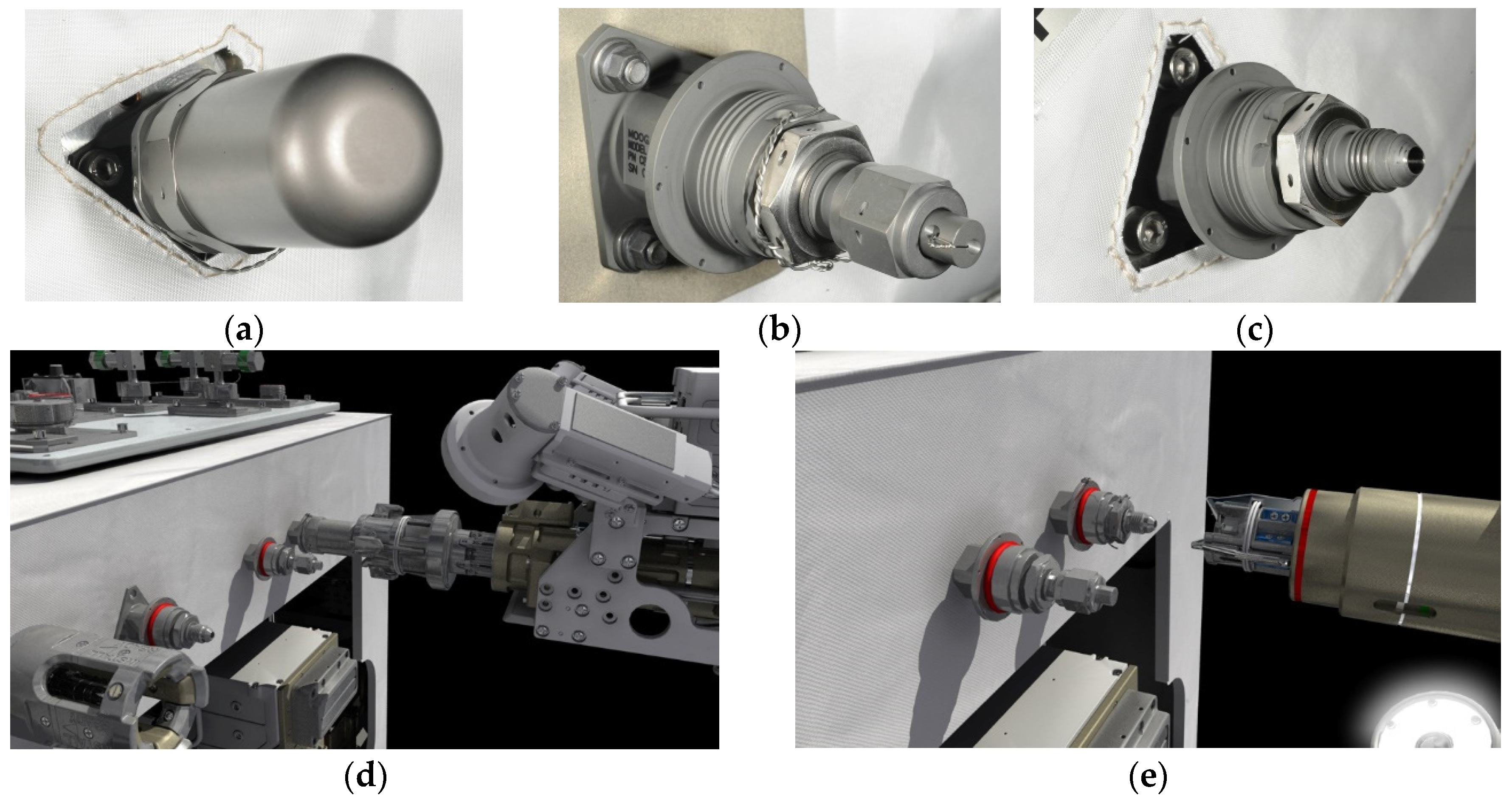
Figure 5.
Space robots with cylindrical center rigid bodies and highly flexible appendages. (a) NASA’s first humanoid space robot, image credit NASA [3] (b) Laboratory flexible rotational spacecraft hub with a very light robotic arm attached on a free-floating on planar air-bearing whose schematic is displayed in subfigure (c).
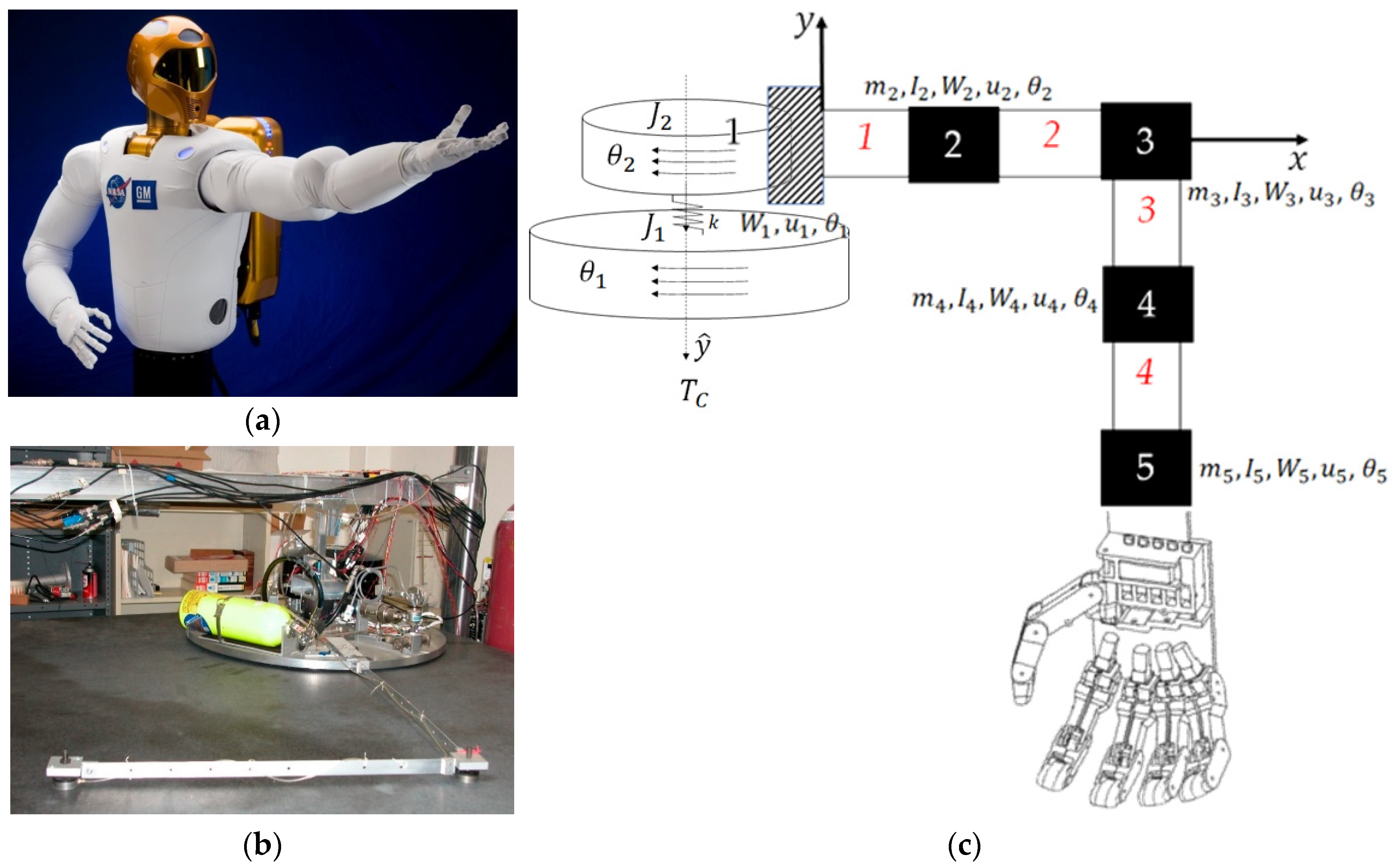
Figure 6.
(a) Laboratory flexible spacecraft robotic arm (very lightweight) attached to a rotational hub free-floating on planar air-bearing. Image used in compliance with image use policy, [2] “U.S. Department of Defense photographs and imagery, unless otherwise noted, are in the public domain.” (b) schematic of center-lined, cylindrical, rigid spacecraft (c) The flexible arm is modeled using the lumped-mass technique where arm mass is distributed to discretized nodes. Images taken from [50] in compliance with respective image use policies. [54].
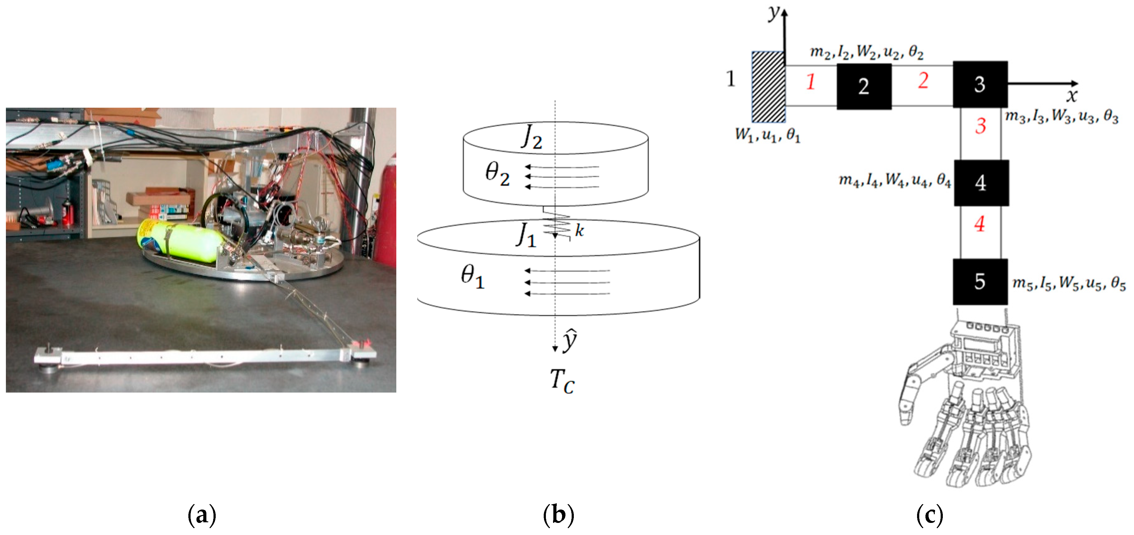
Figure 7.
Topology of simulation created in Simulink®.
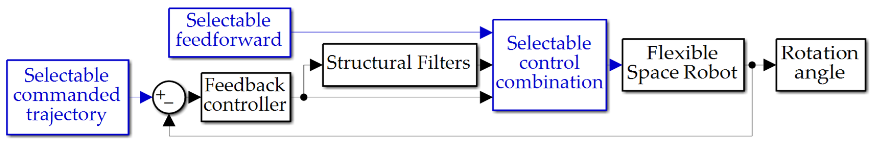
Figure 8.
Topology of simulation created in Simulink®: (a) selectable command trajectory; (b) selectable feedforward; (c) selectable commanded trajectories: thick solid black line is step function, rigid body minimum fuel thin solid green line; bio–inspired whiplash trajectory is the red dashed line, and single sinusoidal commanded trajectory is the dotted blue line (d) feedforward controls: minimum fuel optimal feedforward is the dashed red line, while time-delay input shaped feedforward is the solid blue line in the inset plot.
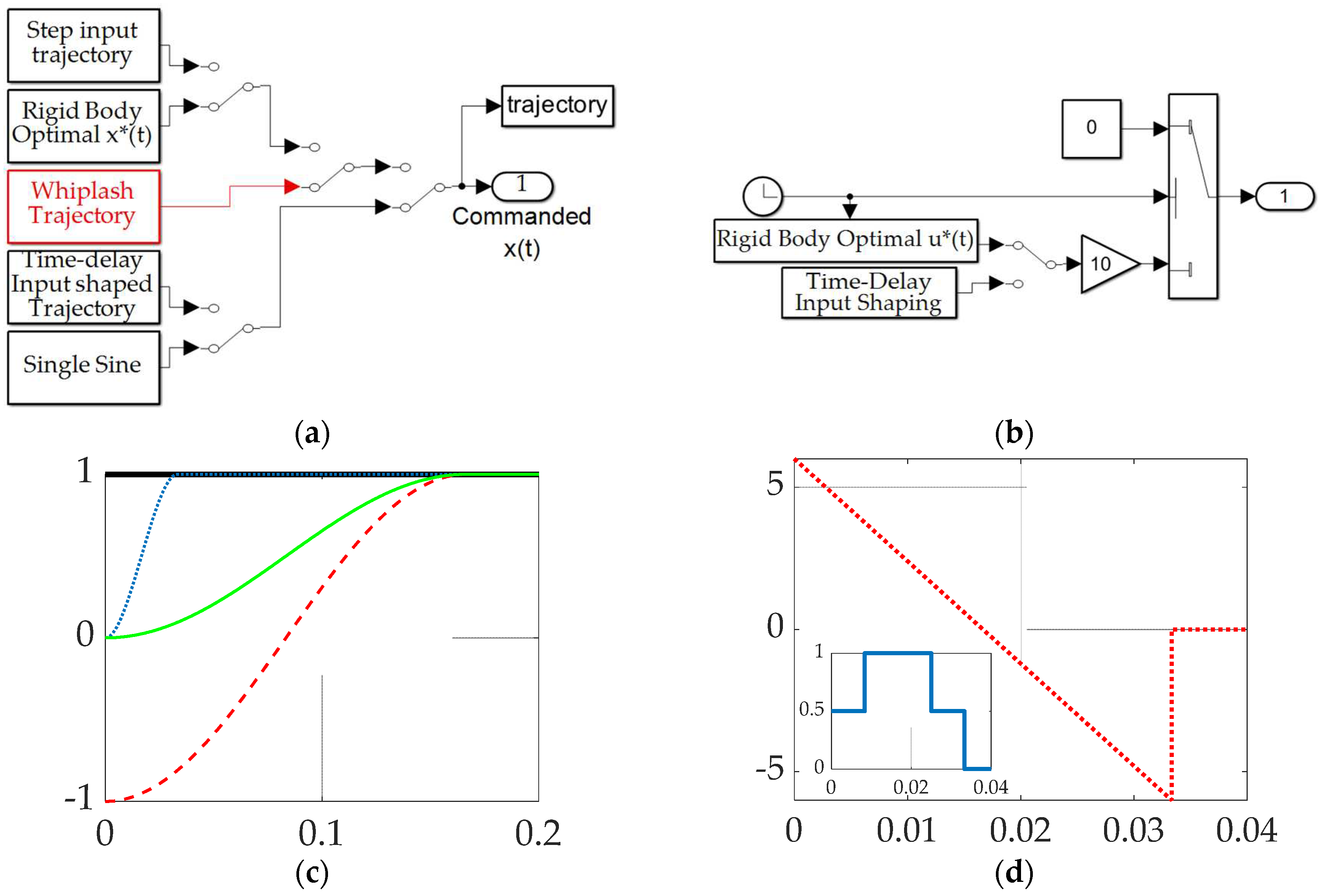
Figure 9.
Topology of simulation created in Simulink®: (a) structural filters; (b) selectable control combination.
Figure 9.
Topology of simulation created in Simulink®: (a) structural filters; (b) selectable control combination.
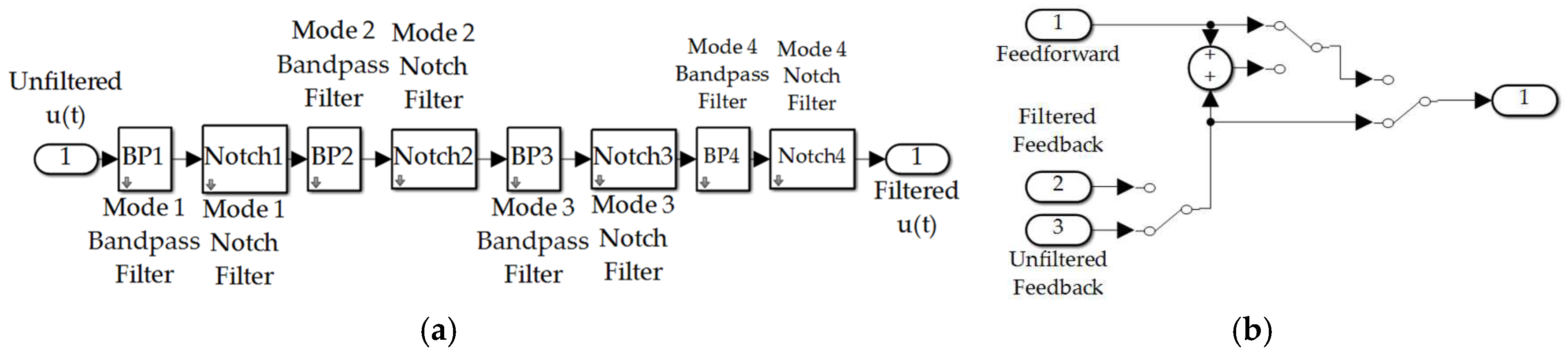
Figure 10.
Feedback filtering for structural resonances and anti-resonances: (a) frequency response plot of unfiltered, PID controlled space robot with decibel frequency on the abscissa and response magnitude on the ordinant; (b) flattened curve, frequency response plot when all four modes are filtered with both bandpass and notch filters with decibel frequency on the abscissa and response magnitude on the ordinant; (c) second-order notch filters optionally applied at resonances with decibel frequency on the abscissa and response magnitude on the ordinant of the right hand subplot with Real (Re) and Imaginary (Im) parts displayed in the left-hand plot; (d) second-order bandpass filters optionally applied to anti-resonances with decibel frequency on the abscissa and response magnitude on the ordinant of the right-hand subplot with Real (Re) and Imaginary (Im) parts displayed in the left-hand plot.
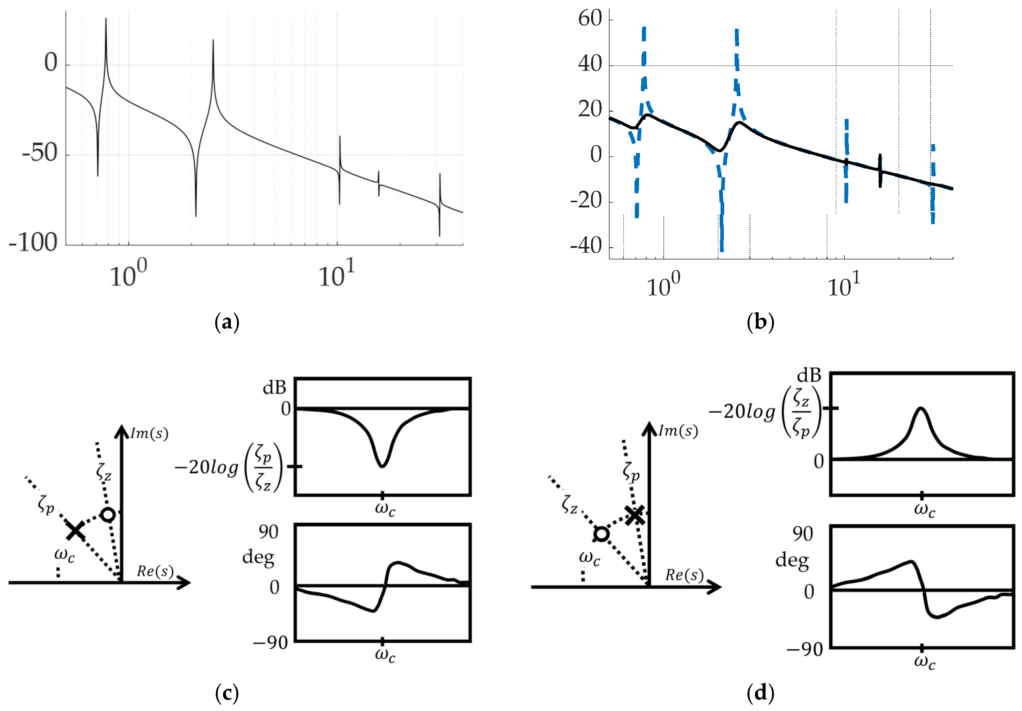
Figure 11.
Trajectory command comparative simulation experiments performed in Simulink®. Solid blue line indicates Step trajectory, no feed-forward, unfiltered; solid black line indicates whiplash trajectory, no feedforward, unfiltered; red dotted line indicates time-delayed input-shaped trajectory, no feedforward, unfiltered (a) control; (b) tracking error, (c) rotation angle. Qualitative results correspond to quantitative figures of merit in Table 6. Rigid body minimum-fuel input trajectory shaping performed so poorly as to not be presentable.
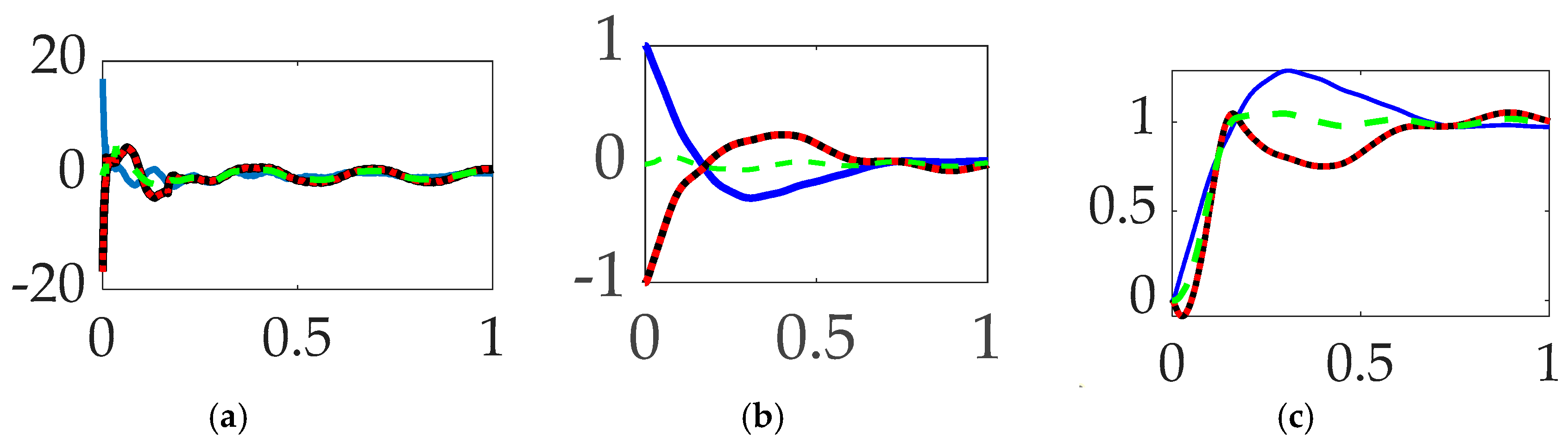
Figure 12.
Selectable feedforward comparative simulation experiments performed in Simulink®. Solid blue line indicates step trajectory, rigid-body optimal feed-forward, unfiltered; solid black line indicates step trajectory, time-delay input shaping feedforward, unfiltered; red dotted line indicates single-sine trajectory, time-delay input shaping feedforward, unfiltered; (a) control; (b) tracking error, (c) rotation angle. Qualitative results correspond to quantitative figures of merit in Table 7. Single-sinusoid trajectory, rigid body optimal feedforward, unfiltered performed so poorly as to not be presentable.
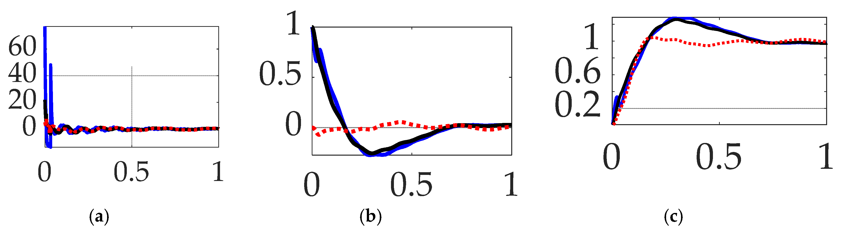
Figure 14.
Selectable mode 2 feedback filtering comparative simulation experiments performed in Simulink®. Solid black line indicates single sine trajectory, no feedforward, mode 2 bandpass filtered; solid blue line indicates single sine trajectory, no feedforward, mode 2 notch filtered; red dotted line indicates single sine trajectory, no feedforward, mode 2 bandpass and notch filtered. (a) control; (b) tracking error, (c) rotation angle. Qualitative results correspond to quantitative figures of merit in Table 10.
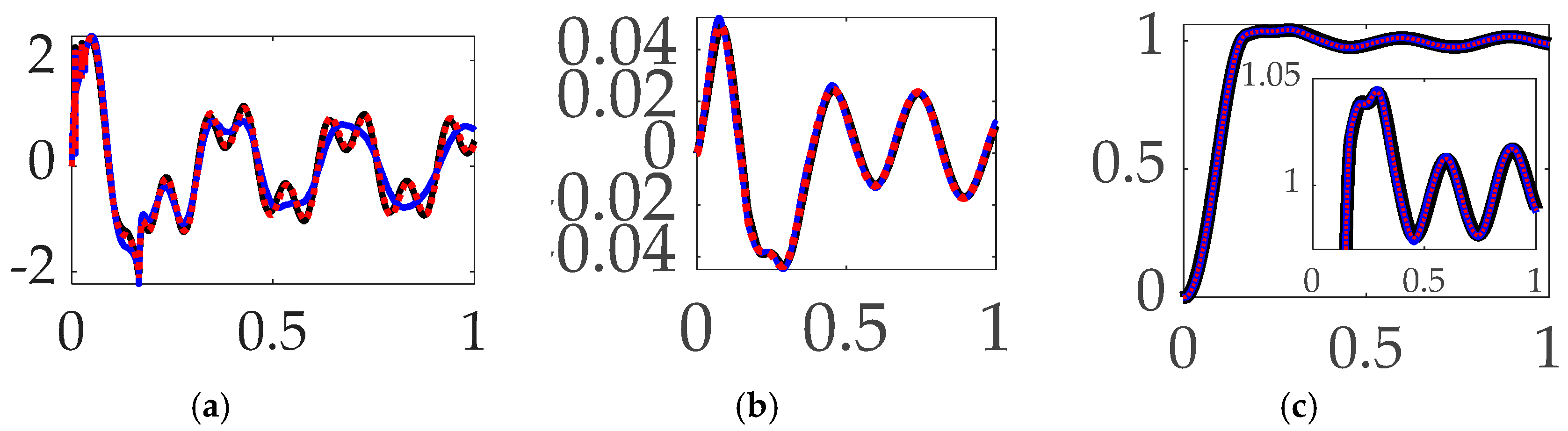
Figure 15.
Selectable mode 3 feedback filtering comparative simulation experiments performed in Simulink®. Solid black line indicates single sine trajectory, no feedforward, mode 3 bandpass filtered; solid blue line indicates single sine trajectory, no feedforward, mode 3 notch filtered; red dotted line indicates single sine trajectory, no feedforward, mode 3 bandpass and notch filtered. (a) control; (b) tracking error, (c) rotation angle. Qualitative results correspond to quantitative figures of merit in Table 11.
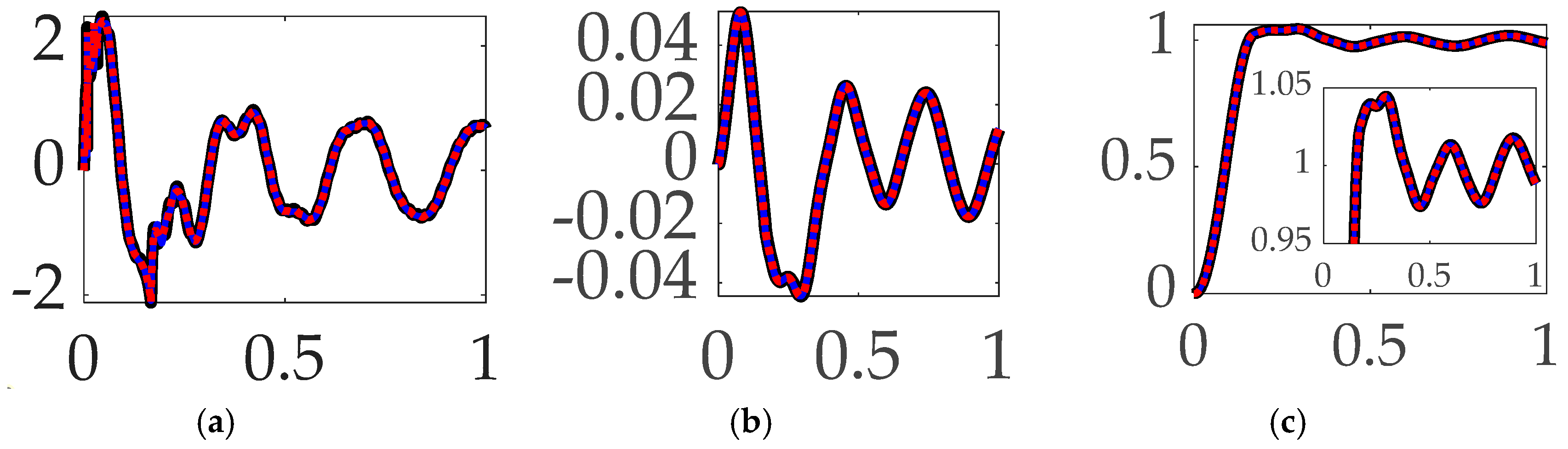
Figure 16.
Selectable mode 4 feedback filtering comparative simulation experiments performed in Simulink®. Solid black line indicates single sine trajectory, no feedforward, mode 4 bandpass filtered; solid blue line indicates single sine trajectory, no feedforward, mode 4 notch filtered; red dotted line indicates single sine trajectory, no feedforward, mode 4 bandpass and notch filtered. (a) control; (b) tracking error, (c) rotation angle. Qualitative results correspond to quantitative figures of merit in Table 12.
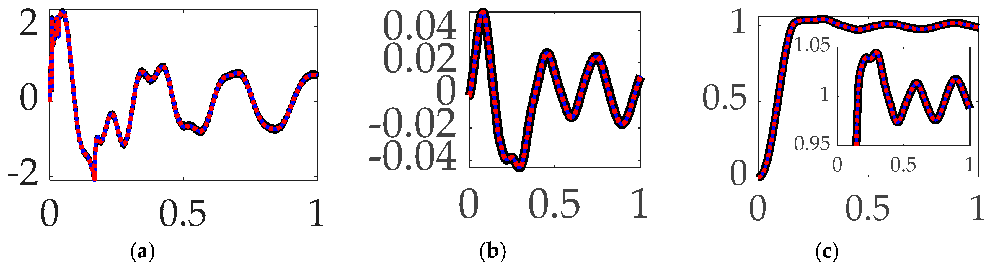
Figure 17.
Selectable modes 1–4 feedback filtering comparative simulation experiments performed in Simulink®. Solid black line indicates single sine trajectory, no feedforward, modes 1–4 bandpass filtered; solid blue line indicates single sine trajectory, no feedforward, modes 1–4 notch filtered. (a) control; (b) tracking error, (c) rotation angle. Qualitative results correspond to quantitative figures of merit in Table 13.
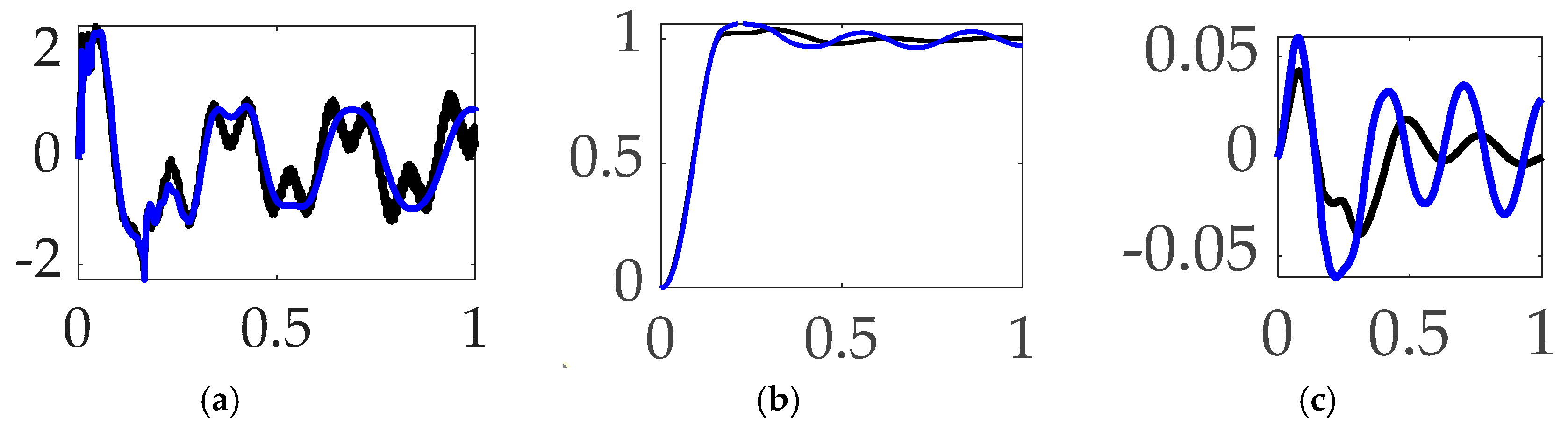
Table 3.
Table of proximal variables and nomenclature 1
| Variable/acronym | Definition |
| Body principal moment of inertia with respect to Z-axis | |
| Angular acceleration of the system rotation angle, | |
| Rigid-elastic coupling term | |
| Acceleration in generalized displacement coordinates | |
| Reaction wheel principal moment of inertia with respect to C, Z axis | |
| Angular acceleration of the reaction wheel rotation angle, | |
| Control torque of the spacecraft reaction wheel | |
| Disturbance torques |
1 Such tables are offered throughout the manuscript to aid readability.
Table 4.
Table of proximal variables and nomenclature 1
|
Variable/ acronym |
Definition |
| Imaginary component of transient response | |
| Real component of transient response | |
| Damping ratio of pole in denominator of equation (12) | |
| Damping ratio of zero in numerator of equation (12) | |
| Center frequency of filter placement | |
| Center frequency of filter pole placement in denominator of equation (12) | |
| Center frequency of filter zero placement in numerator of equation (12) | |
| dB | Decibels |
| Base–10 logarithm | |
| Displacement or rotation expressed in Laplace domain | |
| Control force or torque expressed in Laplace domain | |
| Steady state gain | |
| Maximum phase lead occurring at frequencies determined by & | |
| Maximum gain occurring when |
1 Such tables are offered throughout the manuscript to aid readability.
Table 5.
Trajectory command comparative simulation experiments performed in Simulink®. Quantitative figures of merit correspond to qualitative results in figure 7.
Table 5.
Trajectory command comparative simulation experiments performed in Simulink®. Quantitative figures of merit correspond to qualitative results in figure 7.
| Control methods 1 |
Control effort |
Tracking error mean |
Tracking error deviation |
| Step trajectory, no feedforward, unfiltered | 0.27662 | 0.025967 | 0.29883 |
| Bio–inspired whiplash trajectory, no feedforward, unfiltered | 1.0997 | –0.026376 | 0.2936 |
| Time-delayed input-shaped trajectory, no feedforward, unfiltered | 1.0997 | –0.026376 | –0.27936 |
| Single-sinusoid trajectory, no feedforward, unfiltered | 0.69228 | 0.00052658 | 0.025702 |
1 Rigid body minimum-fuel input trajectory shaping performed so poorly as to not be presentable.
Table 6.
Selectable feedforward comparative simulation experiments performed in Simulink®. Quantitative figures of merit correspond to qualitative results in figure 8.
Table 6.
Selectable feedforward comparative simulation experiments performed in Simulink®. Quantitative figures of merit correspond to qualitative results in figure 8.
| Control methods 1 |
Control effort |
Tracking error mean |
Tracking error deviation |
| Step trajectory, rigid body optimal feedforward, unfiltered | 0.15916 | 0.030193 | 0.29752 |
| Step trajectory, time-delay input-shape feedforward, unfiltered | 0.211539 | 0.026717 | 0.27847 |
| Single-sinusoid trajectory, rigid body optimal feedforward, unfiltered | 294.3845 | 6.1359 | 3.9368 |
| Single-sinusoid trajectory, time-delay input-shape feedforward, unfiltered | 0.61639 | –0.0014197 | 0.026812 |
1 Rigid body minimum-fuel input trajectory shaping performed so poorly as to not be presentable.
Table 7.
Selectable commanded trajectories with filtered feedback (and no feedforward) comparative simulation experiments performed in Simulink®. Quantitative figures of merit correspond to qualitative results in figure 8.
Table 7.
Selectable commanded trajectories with filtered feedback (and no feedforward) comparative simulation experiments performed in Simulink®. Quantitative figures of merit correspond to qualitative results in figure 8.
| Control methods 1 |
Control effort |
Tracking error mean |
Tracking error deviation |
| Step trajectory, no feedforward, filtered feedback | 0.028957 | 0.026908 | 0.30033 |
| Rigid body optimal trajectory, no feedforward, filtered feedback | 3.0251 | 0.0020571 | 0.040348 |
| Bio–inspired whiplash, no feedforward, filtered feedback | 0.70804 | –0.023355 | 0.27816 |
| Single sine trajectory, no feedforward, filtered feedback | 0.70804 | –0.023355 | 0.27816 |
1 Rigid body minimum-fuel input trajectory shaping performed so poorly as to not be presentable
Table 8.
Selectable mode 1 feedback filtering comparative simulation experiments performed in Simulink®. Quantitative figures of merit correspond to qualitative results in figure 9.
Table 8.
Selectable mode 1 feedback filtering comparative simulation experiments performed in Simulink®. Quantitative figures of merit correspond to qualitative results in figure 9.
|
Single sine trajectory, no feedforward, iterated feedback filtering 1 |
Control effort |
Tracking error mean |
Tracking error deviation |
| Mode 1 bandpass filtered | 0.62207 | 0.00046139 | 0.018780 |
| Mode 1 notch filtered | 0.89711 | 0.00046872 | 0.029906 |
| Mode 1 Bandpass and notch filtered | 0.71577 | 0.00058161 | 0.020662 |
Table 9.
Selectable mode 2 feedback filtering comparative simulation experiments performed in Simulink®. Quantitative figures of merit correspond to qualitative results in figure 10.
Table 9.
Selectable mode 2 feedback filtering comparative simulation experiments performed in Simulink®. Quantitative figures of merit correspond to qualitative results in figure 10.
|
Single sine trajectory, no feedforward, iterated feedback filtering 1 |
Control effort |
Tracking error mean |
Tracking error deviation |
| Mode 2 bandpass filtered | 0.47683 | 0.00026452 | 0.022876 |
| Mode 2 notch filtered | 0.68856 | 0.00013103 | 0.023599 |
| Mode 2 Bandpass and notch filtered | 0.41301 | 0.00016559 | 0.023188 |
Table 10.
Selectable mode 3 feedback filtering comparative simulation experiments performed in Simulink®. Quantitative figures of merit correspond to qualitative results in figure 11.
Table 10.
Selectable mode 3 feedback filtering comparative simulation experiments performed in Simulink®. Quantitative figures of merit correspond to qualitative results in figure 11.
|
Single sine trajectory, no feedforward, iterated feedback filtering 1 |
Control effort |
Tracking error mean |
Tracking error deviation |
| Mode 3 bandpass filtered | 0.67211 | 0.00015387 | 0.023116 |
| Mode 3 notch filtered | 0.68804 | 0.00025072 | 0.023377 |
| Mode 3 Bandpass and notch filtered | 0.68986 | 0.00017818 | 0.023274 |
Table 11.
Selectable mode 4 feedback filtering comparative simulation experiments performed in Simulink®. Quantitative figures of merit correspond to qualitative results in figure 12.
Table 11.
Selectable mode 4 feedback filtering comparative simulation experiments performed in Simulink®. Quantitative figures of merit correspond to qualitative results in figure 12.
|
Single sine trajectory, no feedforward, iterated feedback filtering 1 |
Control effort |
Tracking error mean |
Tracking error deviation |
| Mode 4 bandpass filtered | 0.65649 | 0.00075748 | 0.023116 |
| Mode 4 notch filtered | 0.69137 | 0.00330010 | 0.023697 |
| Mode 4 Bandpass and notch filtered | 0.68994 | 0.00094136 | 0.023266 |
Table 12.
Selectable mode feedback filtering comparative simulation experiments performed in Simulink®. Quantitative figures of merit correspond to qualitative results in figure 13.
Table 12.
Selectable mode feedback filtering comparative simulation experiments performed in Simulink®. Quantitative figures of merit correspond to qualitative results in figure 13.
|
Single sine trajectory, no feedforward, iterated feedback filtering 1 |
Control effort |
Tracking error mean |
Tracking error deviation |
| Modes 1–4 bandpass filtered | 0.22672 | 0.0010466 | 0.017807 |
| Modes 1–4 notch filtered | 0.90941 | 0.0038787 | 0.030924 |
Table 13.
Comparison of performance figures of merit: effort and tracking errors.
| Control methods 1 |
Control effort |
Tracking error mean |
Tracking error deviation |
| Bio–inspired whiplash trajectory, no feedforward, unfiltered feedback | 1.0997 | –0.026376 | 0.2936 |
| Bio–inspired whiplash, no feedforward, filtered feedback | 0.70804 | –0.023355 | 0.27816 |
| Rigid body optimal trajectory, no feedforward, filtered feedback | 3.0251 | 0.0020571 | 0.040348 |
| Time-delayed input-shaped trajectory, no feedforward, unfiltered | 1.0997 | –0.026376 | –0.27936 |
| Step trajectory, no feedforward, unfiltered | 0.27662 | 0.025967 | 0.29883 |
| Step trajectory, no feedforward, filtered feedback | 0.028957 | 0.026908 | 0.30033 |
| Step trajectory, rigid body optimal feedforward, unfiltered | 0.15916 | 0.030193 | 0.29752 |
| Single-sinusoid trajectory, no feedforward, unfiltered | 0.69228 | 0.00052658 | 0.025702 |
| Single-sinusoid trajectory, time-delay input-shape feedforward, unfiltered | 0.61639 | –0.0014197 | 0.026812 |
| Sinusoidal trajectories, no feedforward, mode 1 bandpass filtered | 0.62207 | 0.00046139 | 0.018780 |
| Sinusoidal trajectories, no feedforward, mode 2 bandpass filtered | 0.47683 | 0.00026452 | 0.022876 |
| Sinusoidal trajectories, no feedforward, mode 2 notch filtered | 0.68856 | 0.00013103 | 0.023599 |
| Sinusoidal trajectories, no feedforward, mode 2 bandpass & notch filtered | 0.41301 | 0.00016559 | 0.023188 |
| Sinusoidal trajectories, no feedforward, mode 3 bandpass filtered | 0.67211 | 0.00015387 | 0.023116 |
| Sinusoidal trajectories, no feedforward, mode 4 bandpass filtered | 0.65649 | 0.00075748 | 0.023116 |
| Sinusoidal trajectories, no feedforward, mode 1–4 bandpass filtered | 0.22672 | 0.0010466 | 0.017807 |
| Average | 0.658023 | 0.007386 | 0.087848 |
1 Rigid body minimum-fuel input trajectory shaping performed so poorly as to not be presentable
Table 14.
Top three performances in the present study.
| Control methods 1 |
Control effort |
Tracking error mean |
Tracking error deviation |
| Single-sinusoid trajectory, time-delay input-shape feedforward, unfiltered | -6% | -119% | -69% |
| Step trajectory, rigid body optimal feedforward, unfiltered | -96% | 264% | 242% |
| Sinusoidal trajectories, no feedforward, mode 1–4 bandpass filtered | -66% | -86% | -80% |
1 Rigid body minimum-fuel input trajectory shaping performed so poorly as to not be presentable.
Disclaimer/Publisher’s Note: The statements, opinions and data contained in all publications are solely those of the individual author(s) and contributor(s) and not of MDPI and/or the editor(s). MDPI and/or the editor(s) disclaim responsibility for any injury to people or property resulting from any ideas, methods, instructions or products referred to in the content. |
© 2024 by the authors. Licensee MDPI, Basel, Switzerland. This article is an open access article distributed under the terms and conditions of the Creative Commons Attribution (CC BY) license (http://creativecommons.org/licenses/by/4.0/).
Copyright: This open access article is published under a Creative Commons CC BY 4.0 license, which permit the free download, distribution, and reuse, provided that the author and preprint are cited in any reuse.
Submitted:
31 December 2023
Posted:
03 January 2024
You are already at the latest version
Alerts
A peer-reviewed article of this preprint also exists.
This version is not peer-reviewed
Submitted:
31 December 2023
Posted:
03 January 2024
You are already at the latest version
Alerts
Abstract
Controlling robots in space with necessarily low material and structural stiffness is quite challenging at least in part due to the resulting very low structural resonant frequencies. The frequencies are sometimes so low, the vary act of controlling the robot with medium or high bandwidth controllers lead to excitation of resonant vibrations. Biomimetics or biomimicry emulates models, systems, and elements of nature for solving such complex problems. Recent seminal publications have re-introduced the viability of optimal command shaping, and one recent instantiation mimics baseball pitching to propose control of highly flexible space robots. The readership will find a perhaps dizzying array of thirteen decently performing alternatives in the literature but could be left bereft selecting a method(s) deemed to be best suited for a particular application. Bio–inspired control of space robotics is presented in a quite substantial (perhaps not comprehensive) comparison, and the conclusions of the study indicate the top three performing methods based on minimizing control effort (i.e., fuel) usage, tracking error mean, and tracking error deviation include.
Keywords:
Subject: Engineering - Mechanical Engineering
1. Introduction
To accumulate energy, baseball pitchers (Figure 1) “wind up”, initially moving the ball in the opposite direction of the desired destination. The general shape of space robots is not dissimilar to baseball pitchers, and this study evaluates the efficacy of trajectory shaping for space robots inspired by the biomimicry of baseball pitching.
1.1. Broad context and why this study is important
Despite recent demonstrations of operations in space of capabilities at the system level of several autonomous functions [5,6] including robotics, contemporary space operations assessment and action planning rely upon pre-scripted sequences of commands from ground operations personnel. [7] Considering challenging and distant robotics missions (e.g., to Mars) ground operators are unlikely to predict all the likely encounters and physical interactions occurring in parts of space seldomly experienced before.[8] Limited knowledge in complex situations demands autonomy, perceivably establishing a new frontier for space exploration. Another obvious example is utilization of very small spacecraft in cislunar orbits to refuel, repair, and replenish earth-orbiting spacecraft at lower altitudes necessitating grappling potentially unknown masses of uncooperative spacecraft. Extreme fuel efficiency seems mandatory, especially due to the low mass and volume of the underactuated robotic repair spacecraft [8] like those depicted in Figure 2, leading naturally to control minimization as a primary figure of merit. [9]
1.1.1. Cislunar space
A recent primer on cislunar space published by the U.S. Air Force [13] intended to aid the development of expertise, capabilities, plans, and operational concepts. The importance of the orbits manifested in the December 2019 creation of a new branch of the military charged with the duties to defend and protect American space interests. Especially since highly perturbed orbits depart predictable locations; intercept, rendezvous, and proximity operations (depicted in Figure 3) become quite complicated and potentially unpredictable. Cislunar orbits are generally no longer planar and no longer elliptical (certainly not circular), spacecraft positions are no longer easy to articulate geometrically.
1.1.2. Cislunar robotic operations
Actuators for space robots were recently reviewed in [16] highlighting time–delays as a key limiting issue for successful operations, some of which are displayed in Figure 4. A disparate review [17] assembled (over the last three years), subdivided the trends in research development achievements. The reviews focus on two different treatments of modeling uncertainties in hopes of not needing to increase design margins: either increasing the accuracy of parameter discrimination or alternatively developing methods with inherent robustness. The later review [17] emphasized the fact that task performance execution success correlated with onboard computing power.
In the broadest sense, the space robot (like those depicted in Figure 1, Figure 3, and Figure 5) may be considered generically as a cylindrical main body with a robotic appendage attached, leading to both rigid–body and flexible–body treatments. Figure 5 displays two variations on laboratory hardware replicating space robots. Subfigure (b) is the Navy space robot laboratory hardware that serves as the baseline system analyzed in subsequent sections of this manuscript.
Table 1.
Table of proximal variables and nomenclature 1.
| Variable/acronym | Definition | Variable/acronym | Definition |
| Centerline unit vector | Appendage stiffness | ||
| Control torque | Flexible masses and inertias | ||
| Main body inertia mass moment | Flexible inertia mass moment | ||
| Main body rotation angle | Translation & rotation angles |
1 Such tables are offered throughout the manuscript to aid readability.
The literature reveals many mathematical approaches [13] for modeling and also for control, while the readership might be bereft and confused about which method or combinations of methods should be considered for their particular application. This manuscript compares a recently proposed bio–inspired approach to many of the contemporary alternatives.
1.2. Broad review of modeling and control from first–principles to modern instantiations
Modeling can include external and internal constraints on every particle expressed in a Euclidean space [20], or where Newton’s Laws [21] and Euler’s equation [22], may be combined using Chasle’s theorem [23] to define space robot motion states in six degrees of freedom [24]. Control options include both feedback [25] and feedforward (sometimes necessitating system identification) [26] in addition to shaping of the commanded trajectory to ameliorate the deleterious effects of interactions between the control and robot modes that reduce appendage pointing and positioning accuracy. Feedback control is arguably the best understood to adjust robot performance by designing the closed loop system. [27] Well–established, classical techniques include proportional plus integral plus derivative (PID) control [28] emphasizing oscillation design and maintenance of stability following a commanded movement trajectory. A common modern control method used to minimize a performance measure is the linear quadratic regulator [29] ubiquitously applied to linear time–invariant systems, while the presumption for robotic space missions used for refueling and resupply particularly must assume time-variance, since fuels is being relocated and hardware may be removed and replaced. A less frequently first-used control is feedforward elaborated in [30] to be particularly useful if the movements of the space robot are predictable. Feedforward control is also referred to as open–loop control. The recent resurgence of artificial intelligence has not overlooked space robotics, either particularly for medical purposes. [31,32] Robots can be trained by machine learning algorithms to compensate for varying tasks and environments. The internet of things (IoT) is another newly conceived possibility for robot control remotely and monitoring. [33]
Vibration of flexible bodies is strongly driven by the nature of the (impact) excitation or rate of application of external forces. Accordingly, the dynamics of physical contact is important leading to a field of study known as contact dynamics. Such dynamics are modeled using a so–called Hertz model in reference [34] which studied gripping a non–cooperative spacecraft focusing on contact compliance control. The study highlighted the key nature of vibration of flexible spacecraft parts which could lead to repeated continuous collisions. The high flexibility of the robot arms is a key focus of attention for capturing non–cooperative spacecraft. The study presented simulation experiments indicating compliance control seems key to successful performance.
The natural vibrational frequency of the robotic arms is dominated by the arms’ masses and structural stiffness (resistance to motion, either translational or rotational). Tracking control of variable stiffness actuators was studied in reference [35] highlighting robot arm link motor disturbances and variability in actuator stiffnesses (naturally), which may render tracking control schemes ineffective. A mechanism for learning was proposed to compensate for disturbance uncertainties leading to a novel framework for designing controls starting with back–stepping tuning of feedback control, then parameter tuning with finite switching. Validation was offered using computer simulations.
A well–known method called input shaping from the 1990’s has recently been hybridized in reference [36,37] seeking to address vibration residuals in flexible, multi–mode systems. Modal analysis is used to decouple the system by transforming to the reference frame defined by the modal (eigen) vectors. The command is shaped in the diagonalized modal reference frame, where the three contending alternatives were versine (sinusoidal), ramp, or cycloid plus ramped sinusoidal. The methods were compared in simulation experiments which validated high robustness to parameter uncertainty. The general approach is duplicated in this present manuscript comparing bio–inspired whiplash options.
Reference [38] establishes the present study’s comparative benchmark offered by classical control methods augmented with signal processing filters, and the prequel’s benchmark space robot is the same U.S. Navy system whose natural frequencies of vibration are so low as to be excited by even low–bandwidth feedback systems. The utilization of versine shaping proved superior to step commands when the structural filters were designed to achieve system stability margins (classical gain margin and phase margin). Reference [39] is an intermediate sequel investigation on the same navy space robot system, where so–called systems theory methods of Lev Pontryagin were used to develop an open–loop optimal control to minimize maneuver time with quiescent final conditions. The surprising results indicated a “whiplash” shaped command (initially in a direction opposite the commanded terminal state) minimized maneuver time. Results were produced in a commercial, pseudospectral optimization software, and then validation was performed analytically using six necessary conditions of optimization: (1) Hamiltonian minimization condition; (2) adjoint equations; (3) terminal transversality condition; (4) Hamiltonian final value condition; (5) Hamiltonian evolution equation; and lastly (6) Bellman’s principle. Importantly, the bio-mimicking “whiplash” shaping failed to validate one of the six necessary conditions motivating continuing research (including this present manuscript as a new sequel). The biomimicry whiplash control [39] behavior (depicted earlier in this manuscript in Figure 1) is evaluated in this present study applied to shaping the commanded input rather than as a feedforward control.
In addition to high structural flexibility, motor torque limits and joint flexibility are additional considerations emphasized in reference [40] which presented a model–based autonomous generation method for trajectories assuming base excitation and large time–delays for any communications with earth. Computer simulations for verification were presented alongside validation by laboratory experiments on an air–bearing table.
Operationally, highly flexible space robots need to move around large loads of heavy items potentially leading to large tracking errors. Reference [41] proposed damping–stiffness control including joint dynamics in a comprehensive model utilizing Luenberger observers for unmeasurable quantities. Damping was treated as a feedforward (plus gain), while the feedback is used to suppress perturbations. Verification in simulations hinted at a potential ninety–even percent improvement, while laboratory experiments merely validated an eighty–eight percent improvement.
The dynamics (mathematical models) were the focus of reference [42] seeking the proper element number for inclusion in appendage models, where the end effector trajectory was controlled in the feedforward. Sliding mode control including gravity effects was proposed in reference [43] including nonlinear dynamics typically decomposed into separate flexible and rigid subsystems (as was done in the present manuscript’s study), but modelling accuracy strongly drove performance. As the control of highly flexible robotic systems becomes more commonplace, a MATLAB ®/Simulink® toolbox evolved and was presented in reference [44], effectively reducing the coding burden of future investigations.
1.3. The current state of the research field and key references
Reference [34] describes substantial on-going proof-of-concept investigations including space debris removal, life-extension services, on-orbit assembly, and manufacturing, while identifying remaining challenges, particularly simulation of the true six-degrees-of-freedom dynamics of large-scale microgravity operations, especially for robotic systems. The fourth option, so–called “whiplash shaping” is the bio-inspired method of shaping the input commanded trajectories for the space robot.
- Gain stabilization [45]: Tuning of gain to achieve stability of the rigid body mode.
- Classical second-order structural filtering [45]: Second-order filters designed for each chosen resonance and anti-resonance, usually of lowest mode or lowest two modes to ensure stability.
- Rigid body min-fuel input trajectory shaping: Apply control analytically derived from constrained control–minimization boundary value problem solutions.
- Single-frequency trajectory shaping: Fashion commanded trajectory from single sinusoid chosen to avoid mode frequencies of the flexible robot.
- Flatten the curve to improve stability: Use option #2 to compensate for all structural modes seeking to create a magnitude response curve resembling such a curve for a second-order rigid body system (primary motivation remains increased system stability).
- Flatten the curve to improve trajectory tracking: This option is like option #7, except choosing parts of modes (resonance or anti-resonance) to minimize trajectory tracking errors (proposed in this manuscript).
-
Deterministic artificial intelligence: Use physics to define robot self–awareness, while adapting or learning time–varying physical system parameters (e.g., mass, mass moments, stiffness, damping, etc.).
- 9.1
- Self-awareness statements [52]: Use governing equations from physics to exclusively define robot self–awareness, while prescribing necessary trajectories to be tracked (currently only sinusoidal trajectories and control–minimizing trajectories are in the literature).
- 9.2
1.4. Controversial and diverging hypotheses – literature gaps
Two disparate paradigms are evident regarding response magnitude curve shaping: flattening the curve to improve stability [38] versus flattening the curve to improve trajectory tracking (to be addressed in this manuscript).
1.5. Main aim of the work and highlighting of principal conclusions
The goal is to provide the readership an extensive study comparing performances of available options based on multiple figures of merit: necessary fuel expenditure, mean tracking errors, and tracking error deviations.
1.6. Novelties presented
- Commanded trajectory shaping options are compared using control effort and tracking accuracy, and recommendations are offered.
- Feedforward controls are compared using control effort and tracking accuracy, and recommendations are offered.
- Commanded trajectories are compared with filtered feedback and no feedforward using least control effort tracking accuracy, and recommendations are offered.
- Mode 1 filtering options are compared using control effort tracking accuracy, and recommendations are offered.
- Mode 3 filtering options are compared using control effort tracking accuracy, and recommendations are offered.
- Mode 4 filtering options are compared using control effort tracking accuracy, and recommendations are offered.
- Overall recommendations are made for selection of commanded trajectories, feedforward controls, and filtered versus unfiltered feedback.
- The least control effort was achieved with step trajectories, rigid body optimal feedforward control and unfiltered feedback, while recommendations are offered based on tracking accuracy and control effort.
2. Materials and Methods
Section 2.1 introduces modeling of the highly flexible space robot using as a benchmark the free-floating (on an air-bearing) flexible spacecraft simulator at the Naval Postgraduate School depicted in Figure 6, which also depicts system diagrams including both rigid body and flexible robotic appendage. Development of system models (equations) follows next, where the resulting detailed equations are provided in Appendix A. Section 2.2 introduces competing control methodologies and depicts simulation topologies, where detailed simulation codes are provided in Appendix B.
Selectable options include commanded trajectories, feedforward controls, feedback controls, and structural filtering.
2.1. Space robot modeling
The highly flexible space robot laboratory hardware depicted in Figure 6, subfigure (a) is decomposed into a rigid-body base (simulating the near-rigid spacecraft) depicted in subfigure (b) with highly flexible, lightweight robotic appendages modeled using the finite element method in subfigure (c). The first node of the finite element representation is attached to the spacecraft, while flexible elements (mass and stiffnesses) are lumped at subsequent nodes, where Table 2 conveniently defines variables and nomenclature.
Table 2.
Table of proximal variables and nomenclature 1.
| Variable/acronym | Definition | Variable/acronym | Definition |
| Centerline unit vector | Appendage stiffness | ||
| Control torque | Flexible masses and inertias | ||
| Main body inertia mass moment | Flexible inertia mass moment | ||
| Main body rotation angle | Translation & rotation angles |
1 Such tables are offered throughout the manuscript to aid readability.
Newton’s Law for translational motion is expressed in equation (1) where displacements are expressed in coordinates of an inertial reference frame, while similarly Euler’s moment equations are displayed in equation (2). Expressing motion in coordinates of a non-inertial reference frame modifies equations (1) and (2) to equations (3) and (4) respectively. A representative two-node system of equations including internal flexible “spring forces” that resist motion is displayed in equations (5) and (6) respectively for each node, and then assembled into matrix–vector notation in equation (7), where Table 2 conveniently defines variables and nomenclature.
Table 2.
Table of proximal variables and nomenclature 1
| Variable/acronym | Definition |
| , | Externally applied force & torque expressed in inertial coordinates |
| , | Externally applied force & torque expressed in non-inertial coordinates |
| , | Body’s mass & mass moment of inertia |
| Resulting accelerations expressed in inertial coordinates | |
| , | Angular velocity and acceleration vectors |
| ; | Translational velocity and acceleration vectors |
| Flexible member stiffnesses | |
| Assembled matrices of masses and stiffnesses |
1 Such tables are offered throughout the manuscript to aid readability.
Euler’s moment equations in equation (2) are elaborated for the flexible space robot in equation (8) and resembled in equation (9) to more closely resemble the basic expression of Newton’s Law, where variables and nomenclature are conveniently defined in Table 3.
Isolating the first term of equation (9) leads to equation (10), and slight arithmetic leads to equation (11).
Detailed implementation on the flexible space robot depicted in Figure 6 is included in the appendix to aid repeatability. Mode shapes and (constant) natural vibrational frequencies are obtained by spectral decomposition (i.e. the eigenvalue problem). Meanwhile, mass and moments of inertia (locations of mass) vary leading to time–invariant frequenices and shapes, thus motivating the proposals in this manuscript with the anticipation of future research into deterministic artificial intelligence.
2.2. Competing control design methodologies
Many options are available in the literature to the robot designer to control the highly flexible system in space. The immediate prequels elaborated gain stabilization, classical second-order structural filtering, input-shaping, and whiplash compensation (where whiplash trajectory shaping is implemented in this study). Meanwhile, this present manuscript iterates several remaining trajectory shaping options: rigid body minimum-fuel trajectory shaping, single-frequency sinusoid, and options for flattening the magnitude response plot, while establishing some groundwork to prepare for future efforts with deterministic artificial intelligence.
- Gain stabilization.
- Classical second-order structural filtering.
- Input-shaping
- Whiplash compensation.
- Rigid body minimum-fuel input trajectory shaping.
- Single-frequency trajectory shaping
- Flatten the curve to improve stability.
- Flatten the curve to improve trajectory tracking.
-
Deterministic artificial intelligence
- 9.1
- Self-awareness statements
- 9.2
- Adaption or optimal learning
2.3. Selectable options: Trajectories, feedforward, feedback, and filtering
Figure 7 depicts simulations created in SIMULINK® including subsystems for selectable commanded trajectory, selectable feedforward controls, feedback controller, structural filters, and the selection subsystem to activate feedforward, feedback, and structural filtering. Those subsystems are fed to control the flexible space robot’s subsystem in a unit-feedback loop resulting in a displayable rotation angle.
2.3.1. Commanded trajectories
The Simulink® subsystem used to select between commanded trajectories is displayed in Figure 8(a) including ubiquitous step commands, rigid body control–minimizing optimal commands, whiplash compensation, time–delay input shaped trajectories, and single sinusoidal commanded trajectories. Figure 8(b) displays a subsystem used to formulate trajectories that are non-zero only when maneuvering. Meanwhile Figure 8(c) and Figure 8(d) display notion subsystem outputs.
2.3.2. Feedback filtering
Filtering feedback controls is simulated as depicted in Figure 9(a) where iteration of controls is achieved by a subsystem of manually switches depicted in Figure 9(b). Activation of all structural filtering (four bandpass filters placed at the spectral location of four anti-resonances plus four notch filters placed at the spectral location of four resonance frequencies) results in modifying the frequency response magnitude plot depicted in Figure 10 (a) to Figure 10(b), where the spikes and dips of resonance and anti-resonance respectively have been smoothed by the structural filters. Former analysis designed these filters primarily using stability as motivation, while this present research evaluates several figures of merit including trajectory tracking and control usage. Figure 10(c) and (d) respectively depict notion impacts of notch and bandpass filters on the frequency response magnitude plot (i.e., Bode plot’s magnitude), where Table 4 provides convenient definitions of proximal variables and nomenclature.
2.3.3. Feedforward controls
Feedforward controls are strictly taken as the self-awareness statements in deterministic artificial intelligence, where the intension is to use this manuscript as benchmarks for the seminal development of deterministic artificial intelligence for flexible space robotics in the sequel. For example, presently equation (8) is modified to equation (18) by prescribing the motion states (using the chosen commanded trajectories) and using time-invariant estimates of the physical parameters (e.g., mass, mass moments, stiffnesses, and eventually damping). The sequel will modify equation (9) is modified to equation (19) by prescribing the motion states (using the chosen commanded trajectories) and using time-invariant estimates of the physical parameters (e.g., mass, mass moments, stiffnesses, and eventually damping). develop adaption and learning methods for the estimates making them time-varying. Follow-on work will combine the transport theorem in equation (18) with the rigid–elastic coupled system in equation (19) which should permit deterministic artificial intelligence to learn time-varying natural frequencies stemming from time-varying mass, mass moments, stiffnesses, and damping.
Selectable options for designing commanded trajectories, feedforward and feedback controls, and structural filtering were elaborated in section 2.3. Presently concluding the Methods and Materials, section 3 next presents the parameters used in the simulation experiments, and then presents the results of many experiments.
3. Results
This section provides a concise and precise description of the experimental results favoring multi–plots with accompanying tables of comparative figures of merit to aid the readership’s efforts ascertaining the relative efficacy of the approaches presented. Presented next is the data interpretation, as well as the experimental conclusions that can be drawn, culminating in a very large table of thirteen of the best approaches (of the twenty-six approaches iterated), displayed with comparative figures of merit. Mini summaries are provided allowing the reader to discard thoughts of relatively inferior methods, while continuing to the next set of comparisons, eventually narrowing to a grouping of the best available options of those surveyed. The simulation parameters are provided in Table 5 to aid repeatability of the presented results.
3.1. Comparing commanded trajectories with unfiltered feedback
The first options experiments compared disparate options for comparing commanded trajectories with unfiltered, classical PID feedback control. Space robot rotation angles are displayed versus time (scaled to unity) in Figure 11 with corresponding figures of merit in Table 6 revealing obviously superior tracking performance of using single-sinusoidally shaped commanded trajectories without feedforward control and unfiltered classical PID feedback control. Orders-of-magnitude improvements in trajectory tracking mean error and deviations is achievable with more than three-fold increase in fuel utilization (i.e., control effort).
Interim summary. When comparing commanded trajectories, step trajectories surprisingly led to the least control effort, while single-sinusoid trajectories produce the most accurate tracking with 150% more control effort. Bio–inspired whiplash compensation performed essentially as well as time–delayed input–shaping.
3.2. Comparing feedforward controls with unfiltered feedback
Having compared trajectory shaping options in section 3.1, this section includes the results of direct comparison of disparate options for feedforward control in the presence of unfiltered, classical PID feedback control. Figure 12 reveals relatively superlative performance is obtained by using single-sinusoidally shaped, commanded trajectories with time-delay input-shaped feedforward control in the presence of unfiltered classical feedback controls, where figures of merit in Table 7 reveal the increased trajectory tracking performance necessitates a non-trivial increase in fuel expenditure (control effort).
Interim summary. When comparing feedforward controls, rigid body optimal feedforward with step trajectory command surprisingly led to the least control effort, while time-delay input-shaped feedforward with single-sinusoid trajectories commanded produced the most accurate tracking with 280% more control effort.
3.3. Comparing commanded trajectories with filtered feedback
Having discerned the advantages of single-sinusoidally shaped, commanded trajectories and time-delay input-shaped feedforward control, this section repeats the comparison in Section 3.1 (which included only unfiltered feedback), but this time iterates the options when structural filters are use. Figure 13 reveals the lowest control effort (i.e., fuel usage) with nominal tracking performance using unshaped step commands, no feedforward controls with structurally filtered feedback; however, substantially improved target tracking performance is achievable at using higher control efforts by commanding optimal (fuel-minimizing) trajectories that are constrained by rigid-body dynamics equations.
Figure 13.
Selectable commanded trajectory comparative simulation experiments performed in Simulink®. Solid blue line indicates step trajectory, no feedforward, filtered feedback; solid black line indicates rigid body optimal trajectory, no feedforward, filtered feedback; red dotted line indicates whiplash trajectory, no feedforward, filtered feedback; and green dashed line indicates single sine trajectory, no feedforward, filtered feedback (a) control; (b) tracking error, (c) rotation angle. Qualitative results correspond to quantitative figures of merit in Table 8.
Figure 13.
Selectable commanded trajectory comparative simulation experiments performed in Simulink®. Solid blue line indicates step trajectory, no feedforward, filtered feedback; solid black line indicates rigid body optimal trajectory, no feedforward, filtered feedback; red dotted line indicates whiplash trajectory, no feedforward, filtered feedback; and green dashed line indicates single sine trajectory, no feedforward, filtered feedback (a) control; (b) tracking error, (c) rotation angle. Qualitative results correspond to quantitative figures of merit in Table 8.
Interim summary. When comparing commanded trajectories with filtered feedback and no feedforward, step trajectory commands surprisingly led to the least control effort, while rigid body optimal trajectories achieved an order of magnitude higher accuracy with 2345% more control effort.
3.4. Comparing mode 1 filtering with single-sinusoidal trajectories and no feedforward
The final sections of the manuscript present experiments with iterated structural filtering: mode 1, mode 2, mode 3, mode 4, and then all of modes 1–4. Single-sinusoidally commanded trajectories are carried over from Section 3.1, Section 3.2 and Section 3.3, identified as a burgeoning best practice. This section iterates compensation of the lowest (first) flexible mode by sequentially compensating for the anti-resonance, the resonance, and then both modal features. The prequel literature predominantly designs structural filters for the sake of stability, often leading to emphasizing notch filtering the first resonant peak, while the results here (designed for target tracking performance rather than stability) indicate superior performance is obtainable by only compensating for the first anti-resonance frequency. This assertion is buttressed by the qualitative results in Figure 13 whose quantitative companion is displayed in Table 9’s display of meaningful performance figures of merit.
Figure 13.
Selectable mode 1 feedback filtering comparative simulation experiments performed in Simulink®. Solid black line indicates single sine trajectory, no feedforward, mode 1 bandpass filtered; solid blue line indicates single sine trajectory, no feedforward, mode 1 notch filtered; red dotted line indicates single sine trajectory, no feedforward, mode 1 bandpass and notch filtered. (a) control; (b) tracking error, (c) rotation angle. Qualitative results correspond to quantitative figures of merit in Table 9.
Figure 13.
Selectable mode 1 feedback filtering comparative simulation experiments performed in Simulink®. Solid black line indicates single sine trajectory, no feedforward, mode 1 bandpass filtered; solid blue line indicates single sine trajectory, no feedforward, mode 1 notch filtered; red dotted line indicates single sine trajectory, no feedforward, mode 1 bandpass and notch filtered. (a) control; (b) tracking error, (c) rotation angle. Qualitative results correspond to quantitative figures of merit in Table 9.
Interim summary. When comparing mode 1 filtering options bandpass only not-surprisingly led to the least control effort, but surprisingly also produced the most accurate tracking.
3.5. Comparing mode 2 filtering with single-sinusoidal trajectories and no feedforward
Similar to section 3.4’s comparison of the compensation of the first mode, this section sequentially compensates for the second mode’s anti-resonance, resonance, and then both modal components. The results are displayed in Figure 14 which reveal marginal qualitative differences that are validated by quantitative results in Table 10.
Interim summary. When comparing mode 2 filtering options bandpass and notch led to the least control effort, but surprisingly accurate tracking results were inconsistent.
3.6. Comparing mode 3 filtering with single-sinusoidal trajectories and no feedforward
Continuing the evaluation to the third structural mode, like paragraphs 3.4 and 3.5, this paragraph presents the experiment results of sequentially compensating for the third mode’s anti-resonance, resonance, and then both modal components. Similar to the results achieved compensating for the first resonant mode, compensation of the third mode’s bandpass alone proved superior. In this instance, the results are clearly marginal, evidenced in the qualitative displays of Figure 15, where the small differences are quantitatively displayed in Table 11.
Interim summary. When comparing mode 3 filtering options bandpass led to the least control effort and also produced the most accurate tracking accuracy.
3.7. Comparing mode 4 filtering with single-sinusoidal trajectories and no feedforward
The three immediately preceding sections of this manuscript iteratively investigated the first three structural modes, while this paragraph iteratively compensates for the modal components of the fourth structural mode: the anti-resonance, resonance, and then both. Figure 16 (like Figure 15’s qualitative results) reveal marginal results, where inspection of the quantitative results in Table 12 indicate the repeated trend: compensation for the anti-resonance has the largest impact on target tracking errors.
Interim summary. When comparing mode 4 filtering options bandpass led to the least control effort and also produced the most accurate tracking accuracy.
3.8. Comparing modes 1–4 filtering with single-sinusoidal trajectories and no feedforward
Section 3.1, Section 3.2, Section 3.3, Section 3.4, Section 3.5, Section 3.6 and Section 3.7 iteratively examined compensation of individual modal components, while this section simultaneously compensates for all four modes’ anti-resonances followed by all round modes’ resonances. Definite differences are immediately apparent in Figure 17, where the quantitative figures of merit in Table 13 re-validate the discoveries of Section 3.1, Section 3.2, Section 3.3, Section 3.4, Section 3.5, Section 3.6 and Section 3.7: compensation for the anti-resonance alone has the biggest impact on target tracking performance (with a reminder: the opposite result comes from compensating for stability rather than tracking performance).
Interim summary. When comparing modes 1–4 filtering options bandpass not only led to the least control effort but also produced the most accurate tracking accuracy.
3.9. Comparison of the best options studies
This paragraph assembles and compares thirteen common options for controlling highly flexible space robotics providing advice to the readership: should filtered or unfiltered feedback be used? Should feedforward techniques be considered? Is command trajectory shaping effective? From the experiments presented, interesting mixtures of options illustrate efficacy. Table 13 contains a summary of figures of merit achieved by thirteen disparate combinations of available options: input shaping, feedforward and/or feedback control and optional structural filtering.
Interim summary. The least control effort was achieved with step trajectories, rigid body optimal feedforward control and unfiltered feedback, and the effort was 75% less than the average. The best mean tracking error was achieved with sinusoidal trajectories, no feedforward, mode 2 notch filtered, and the tracking error mean was 98% better than the average, while the control effort was 330% higher than the minimum available option. The best tracking error deviation was achieved with sinusoidal trajectories, no feedforward, mode 1–4 bandpass filtered, and the tracking error deviation was 80% better than the average, while the control effort was 42% higher than the minimum available option.
4. Discussion
This section discusses the results and how they can be interpreted from the perspective of previous studies and of the working hypotheses. The findings and their implications are discussed in the broadest context possible. Future research directions are also highlighted. The top seven revelations follow:
- Bio–inspired trajectory shaping (modified from a time–minimization control per [39]) seems confounded in the presence of classical, unfiltered feedback. While the technique performed well, it was not the exemplary option when compared to the multitude of other available options examined.
- When comparing commanded trajectories, step trajectories surprisingly led to the least control effort, while single-sinusoid trajectories produce the most accurate tracking with 150% more control effort. The bio–inspired whiplash shaping was optimized in the cited literature for minimum time in a feedforward control sense, while this sequel reveals the solution is not minimum effort (fuel), nor minimum time in the presence of feedback.
- When comparing feedforward controls, rigid body optimal feedforward with step trajectory command surprisingly led to the least control effort, while time-delay input-shaped feedforward with single-sinusoid trajectories commanded produced the most accurate tracking with 280% more control effort.
- When comparing commanded trajectories with filtered feedback and no feedforward, step trajectory commands surprisingly led to the least control effort, while rigid body optimal trajectories achieved an order of magnitude higher accuracy with 2345% more control effort.
- When comparing mode 1 filtering options bandpass alone not-surprisingly led to the least control effort, but surprisingly also produced the most accurate tracking.
- When comparing mode 3 filtering options bandpass led to the least control effort and also produced the most accurate tracking accuracy.
- When comparing mode 4 filtering options bandpass led to the least control effort and also produced the most accurate tracking accuracy.
- The least control effort was achieved with step trajectories, rigid body optimal feedforward control and unfiltered feedback, and the effort was 75% less than the average. The best mean tracking error was achieved with sinusoidal trajectories, no feedforward, mode 2 notch filtered, and the tracking error mean was 98% better than the average, while the control effort was 330% higher than the minimum available option. The best tracking error deviation was achieved with sinusoidal trajectories, no feedforward, mode 1–4 bandpass filtered, and the tracking error deviation was 80% better than the average, while the control effort was 42% higher than the minimum available option.
4.1. Results in broad context
Reference [38] studied iterations of classical feedback control augmented with structural filters taken from the discipline of signal processing (e.g., notch filters and bandpass filters), where the options were iterated to maximize classical stability margins (i.e., gain margin and phase margin). Alternatively, the feedback–related sections of this investigation iterated the same options towards a goal of minimizing trajectory tracking error.
Meanwhile, reference [39] open loop optimal feedforward was provided for minimizing the maneuver time without the presence of feedback or filtering. The results were bio–inspired, but the time minimizing results did not rank in the top three performances in the present study seeking the best options for target tracking error.
4.2. Controversial or unexpected results
While reference [38] indicates the best selection of options to maximize classical stability margins (i.e., gain margin and phase margin) was attained by only compensating for the first complete flexible mode (resonance and anti-resonance) with notch and bandpass filters, respectively, with step commands shaped by novel single-sinusoidal trajectories.
Meanwhile, the results presented in the present manuscript indicate split results based on lowest control effort, least tracking error mean, or tracking error deviation.
4.2.1. Best control effort
For the best trajectory tracking measured by least control effort, unfiltered feedback (no notch or bandpass filters) is preferred when unshaped step inputs feed rigid body optimal feedforward controls (as displayed in Table 14.
4.2.2. Best tracking error mean
For the best trajectory tracking measured by lowest mean, unfiltered feedback (no notch or bandpass filters) is preferred step inputs and rigid body optimal feedforward controls (as displayed in Table 14.
4.2.3. Best tracking error deviation
For the best trajectory tracking measured by lowest deviation, sinusoidally–shaped commanded trajectories with no feedforward but bandpass–only filtering of modes (as displayed in Table 14.
4.3. Recommended future reseach
A major motivation of the present study is to evaluate the various efficacies of disparate input shaping techniques available to the recently proposed deterministic artificial intelligence method that necessitates such.
4.3.1. Deterministic artificial intelligence
Following the introduction of the feedforward by Cooper/Heidlauf in 2017 [52] applied to chaotic circuits, the seminal introduction of the technique (including both 2–norm optimal feedforward and feedback) was offered by Smeresky/Rizzo [53] applied to spacecraft, despite not yet bearing the name of the technique back in the year 2020. Following the publication of [38,39] comparative prequels, the natural sequels are recommended here as future research: Utilize the trajectories evaluated here for spacecraft as inputs to the deterministic artificial intelligence method to formulate a seminal offering applied to highly flexible space robotics.
Funding
This research received no external funding.
Data Availability Statement
Data supporting reported results can be obtained by contacting the corresponding author.
Conflicts of Interest
The author declares no conflict of interest.
Appendix A. Elaboration of modal system identification on the flexible robot system
Substitute into equation (19):
Recall the expressions for the rigid elastic coupling using modal coordinates: where ’s are mode shapes from finite element analysis using the eigenvalues of K/m (stiffness/mass). The system stiffness matrix is included in Table A1 and mass matrix in Table A2 result in the natural frequencies and mode shapes for the flexible system in Table A3 and Table A4.
Table A1.
Stiffness matrix [K].
| W2 | θ2 | W3 | θ3 | W4 | θ4 | W5 | θ5 | U6 | θ6 | u7 | θ7 | u8 | θ8 | |
| W2 | 958.8179 | 0.0000 | -479.409 | 59.9261 | 0 | 0 | 0 | 0 | 0 | 0 | 0 | 0 | 0 | 0 |
| θ2 | 0.0000 | 19.9754 | -59.9261 | 4.9938 | 0 | 0 | 0 | 0 | 0 | 0 | 0 | 0 | 0 | 0 |
| W3 | -479.409 | -59.926 | 958.8179 | 0.0000 | -479.409 | 59.9261 | 0 | 0 | 0 | 0 | 0 | 0 | 0 | 0 |
| θ3 | 59.9261 | 4.9938 | 0.0000 | 19.9754 | -59.9261 | 4.9938 | 0 | 0 | 0 | 0 | 0 | 0 | 0 | 0 |
| W4 | 0 | 0 | -479.409 | -59.926 | 958.8179 | 0.0000 | -479.409 | 59.9261 | 0 | 0 | 0 | 0 | 0 | 0 |
| θ4 | 0 | 0 | 59.9261 | 4.9938 | 0.0000 | 19.9754 | -59.9261 | 4.9938 | 0 | 0 | 0 | 0 | 0 | 0 |
| W5 | 0 | 0 | 0 | 0 | -479.409 | -59.926 | 479.409 | -59.926 | 0 | 0 | 0 | 0 | 0 | 0 |
| θ5 | 0 | 0 | 0 | 0 | 59.9261 | 4.9938 | -59.9261 | 19.9754 | -59.9261 | 4.9938 | 0 | 0 | 0 | 0 |
| U6 | 0 | 0 | 0 | 0 | 0 | 0 | 0 | -59.926 | 958.8179 | 0.0000 | -479.409 | 59.9261 | 0 | 0 |
| θ6 | 0 | 0 | 0 | 0 | 0 | 0 | 0 | 4.9938 | 0.0000 | 19.9754 | -59.9261 | 4.9938 | 0 | 0 |
| U7 | 0 | 0 | 0 | 0 | 0 | 0 | 0 | 0 | -479.409 | -59.926 | 958.8179 | 0.0000 | -479.409 | 59.9261 |
| θ7 | 0 | 0 | 0 | 0 | 0 | 0 | 0 | 0 | 59.9261 | 4.9938 | 0.0000 | 19.9754 | -59.9261 | 4.9938 |
| U8 | 0 | 0 | 0 | 0 | 0 | 0 | 0 | 0 | 0 | 0 | -479.409 | -59.926 | 479.4089 | -59.926 |
| θ8 | 0 | 0 | 0 | 0 | 0 | 0 | 0 | 0 | 0 | 0 | 59.9261 | 4.9938 | -59.9261 | 9.9877 |
1 Notice state sequence alternates translation, then rotation at each node.
Table A2.
Mass matrix [M]
| Mass | W2 | θ2 | W3 | θ3 | W4 | θ4 | W5 | θ5 | U6 | θ6 | u7 | θ7 | u8 | θ8 |
| W2 | 0.4761 | 0.0000 | 0.0037 | -0.0002 | 0 | 0 | 0 | 0 | 0 | 0 | 0 | 0 | 0 | 0 |
| θ2 | 0.0000 | 0.0000 | 0.0002 | -0.0001 | 0 | 0 | 0 | 0 | 0 | 0 | 0 | 0 | 0 | 0 |
| W3 | 0.0037 | 0.0002 | 4.76E-01 | 0.0000 | 0.0037 | -0.0002 | 0 | 0 | 0 | 0 | 0 | 0 | 0 | 0 |
| θ3 | -0.0002 | -0.0001 | 0.0000 | 0.0000 | 0.0002 | -0.0001 | 0 | 0 | 0 | 0 | 0 | 0 | 0 | 0 |
| W4 | 0 | 0 | 0.0037 | 0.0002 | 0.4761 | 0.0000 | 0.0037 | -0.0002 | 0 | 0 | 0 | 0 | 0 | 0 |
| θ4 | 0 | 0 | -0.0002 | -0.0001 | 0.0000 | 0.0000 | 0.0002 | -0.0001 | 0 | 0 | 0 | 0 | 0 | 0 |
| W5 | 0 | 0 | 0 | 0 | 0.0037 | 0.0002 | 2.63E+00 | -0.0004 | 0 | 0 | 0 | 0 | 0 | 0 |
| θ5 | 0 | 0 | 0 | 0 | -0.0002 | -0.0001 | -0.0004 | 0.0000 | 0.0002 | -0.0001 | 0 | 0 | 0 | 0 |
| U6 | 0 | 0 | 0 | 0 | 0 | 0 | 0 | 0.0002 | 4.76E-01 | 0.0000 | 0.0037 | -0.0002 | 0 | 0 |
| θ6 | 0 | 0 | 0 | 0 | 0 | 0 | 0 | -0.0001 | 0.00E+00 | 0.0000 | 0.0002 | -0.0001 | 0 | 0 |
| U7 | 0 | 0 | 0 | 0 | 0 | 0 | 0 | 0 | 0.0037 | 0.0002 | 0.4761 | 0.0000 | 0.0037 | -0.0002 |
| θ7 | 0 | 0 | 0 | 0 | 0 | 0 | 0 | 0 | -0.0002 | -0.0001 | 0.0000 | 0.0000 | 0.0002 | -0.0001 |
| U8 | 0 | 0 | 0 | 0 | 0 | 0 | 0 | 0 | 0 | 0 | 0.0037 | 0.0002 | 4.66E-01 | -0.0004 |
| θ8 | 0 | 0 | 0 | 0 | 0 | 0 | 0 | 0 | 0 | 0 | -0.0002 | -0.0001 | -0.0004 | 0.0000 |
1 Notice state sequence alternates translation, then rotation at each node.
Table A3.
Natural frequencies, [rad/s]
| 1809.5 | 1415.5 | 1042.2 | 774.3 | 596.8 |
| 478.8 | 410.9 | 54.9 | 43.7 | 30.9 |
| 15.8 | 10.2 | 0.7 | 2.1 |
1 corresponding to mode shapes in Table 5.
Table A4.
Normalized mode shapes [x104]
| -1 | 3 | 2 | 0 | -3 | -5 | 3 | 1501 | 383 | 1037 | 443 | -692 | 181 | 240 |
| -1097 | 3080 | 4481 | 4992 | 4505 | 3173 | -1154 | -4544 | -136 | 2388 | 2221 | 4049 | 1395 | 1669 |
| -1 | 1 | -3 | -7 | -5 | 1 | -2 | -1569 | -215 | 204 | 667 | 1425 | -670 | -712 |
| -2158 | 4857 | 3958 | 28 | -3814 | -4883 | 2208 | -943 | -2040 | -7064 | -867 | 912 | -2460 | -1864 |
| -1 | -1 | -5 | 0 | 7 | 3 | 2 | 1296 | -125 | -1076 | 125 | 995 | -1385 | -1057 |
| -3111 | 4495 | -1058 | -4992 | -1185 | 4481 | -3142 | 5806 | 2118 | 368 | -2572 | 4061 | -3204 | -683 |
| 0 | 0 | 0 | 1 | 1 | -1 | 1 | -99 | 30 | 113 | -105 | 248 | 2247 | 954 |
| -3902 | 2199 | -4861 | -47 | 4875 | -2071 | 3937 | -4288 | -3426 | 4504 | 1878 | 4753 | -3652 | 1689 |
| 0 | -3 | 4 | 0 | -6 | 6 | 1 | 536 | -918 | 135 | 898 | 754 | -946 | 736 |
| -4493 | -1062 | -3138 | 4985 | -3062 | -1232 | -4519 | 815 | 2292 | -2423 | 3091 | 891 | -3893 | 3998 |
| 0 | 2 | 5 | -7 | 7 | -4 | 0 | -294 | 753 | 446 | 880 | 410 | -1936 | 1905 |
| -4872 | -3903 | 2129 | 75 | -2232 | 3920 | 4832 | -2471 | 3385 | -210 | -3658 | 3392 | -4013 | 5178 |
| -1 | -2 | 2 | -3 | 4 | -5 | -6 | 90 | -261 | 192 | -699 | -732 | -2945 | 3254 |
| -5031 | -5052 | 5012 | -5030 | 5062 | -4984 | -4965 | 3580 | -7823 | 3941 | -7649 | -5153 | -4046 | 5502 |
Figure A1.
Normalized mode shapes (modal coordinates) displayed in physical coordinates with normalized length on the abscissa in meters and displacements in meters on the ordinant.
Figure A1.
Normalized mode shapes (modal coordinates) displayed in physical coordinates with normalized length on the abscissa in meters and displacements in meters on the ordinant.
A.1. Equations of Motion in Standard State Space Form
Finite element analysis performed in MATLAB® (code is included in the appendix) generates the mode shapes used to calculate the rigid-elastic coupling terms. The program outputs the flexible system [A], [B], [C], and [D] matrices of the standard state space form. The results are:
Given these equations, the resultant state space matrices are:
Table A5.
State Space [A] matrix.
| 1 | 2 | 3 | 4 | 5 | 6 | 7 | 8 | 9 | 10 | 11 | 12 | |
| 1 | 0 | 0 | 0 | 0 | 0 | 0 | 1 | 0 | 0 | 0 | 0 | 0 |
| 2 | 0 | 0 | 0 | 0 | 0 | 0 | 0 | 1 | 0 | 0 | 0 | 0 |
| 3 | 0 | 0 | 0 | 0 | 0 | 0 | 0 | 0 | 1 | 0 | 0 | 0 |
| 4 | 0 | 0 | 0 | 0 | 0 | 0 | 0 | 0 | 0 | 1 | 0 | 0 |
| 5 | 0 | 0 | 0 | 0 | 0 | 0 | 0 | 0 | 0 | 0 | 1 | 0 |
| 6 | 0 | 0 | 0 | 0 | 0 | 0 | 0 | 0 | 0 | 0 | 0 | 1 |
| 7 | 0 | 0.099 | -1.064 | -3.382 | -0.736 | -26.635 | 0 | 1.392E-04 | -5.066E-04 | -3.298E-04 | -4.662E-05 | -8.609E-04 |
| 8 | 0 | -0.659 | 1.642 | 5.218 | 1.136 | 41.100 | 0 | -9.264E-04 | 7.817E-04 | 5.088E-04 | 7.194E-05 | 1.328E-03 |
| 9 | 0 | 0.188 | -6.435 | -6.433 | -1.401 | -50.670 | 0 | 2.649E-04 | -3.064E-03 | -6.273E-04 | -8.869E-05 | -1.638E-03 |
| 10 | 0 | 0.025 | -0.270 | -106.024 | -0.187 | -6.755 | 0 | 3.531E-05 | -1.285E-04 | -1.034E-02 | -1.182E-05 | -2.183E-04 |
| 11 | 0 | 0.002 | -0.025 | -0.079 | -249.447 | -0.620 | 0 | 3.241E-06 | -1.179E-05 | -7.677E-06 | -1.579E-02 | -2.004E-05 |
| 12 | 0 | 0.022 | -0.233 | -0.742 | -0.162 | -962.998 | 0 | 3.055E-05 | -1.112E-04 | -7.237E-05 | -1.023E-05 | -3.113E-02 |
1 Flexible states where base (rigid body) rotation is controlled.
Appendix B. Initialization Function callbacks for simulation
| clear all; close all; clc; | |||||||
| %This block of code establishes the properties of each beam element a=0.0254; b=0.0016; L=0.25; E=72*10^9; I=a*b^3/12; Li=[12 6*L -12 6*L;6*L 4*L^2 -6*L 2*L^2;-12 -6*L 12 -6*L;6*L 2*L^2 -6*L 4*L^2]; k_beam=E*I/L^3*[Li]; | |||||||
| rho_beam=2.8*10^3; A_beam=a*b; mb=rho_beam*A_beam; |
%Beam density kg/m^3 %Beam cross sectional area %Beam mass per unit length |
||||||
| %This block creates the empty stiffness matrix [k] k=zeros(14,14); | |||||||
| % This block fills in the stiffness matrix components | |||||||
| % Row 1 components start at index=1 k(1,1)=k_beam(3,3)+k_beam(1,1); k(1,2)=k_beam(3,4)+k_beam(1,2); k(1,3)=k_beam(1,3); k(1,4)=k_beam(1,4); |
% Row 2 components start at index=15 k(2,1)=k_beam(4,3)+k_beam(2,1); k(2,2)=k_beam(4,4)+k_beam(2,2); k(2,3)=k_beam(2,3); k(2,4)=k_beam(2,4); |
||||||
| % Row 3 components start at index=29 k(3,1)=k_beam(3,1); k(3,2)=k_beam(3,2); k(3,3)=k_beam(3,3)+k_beam(1,1); k(3,4)=k_beam(3,4)+k_beam(1,2); k(3,5)=k_beam(1,3); k(3,6)=k_beam(1,4); |
% Row 4 components start at index=43 k(4,1)=k_beam(4,1); k(4,2)=k_beam(4,2); k(4,3)=k_beam(4,3)+k_beam(2,1); k(4,4)=k_beam(4,4)+k_beam(2,2); k(4,5)=k_beam(2,3); k(4,6)=k_beam(2,4); |
||||||
| % Row 5 components start at index=59 k(5,3)=k_beam(3,1); k(5,4)=k_beam(3,2); k(5,5)=k_beam(3,3)+k_beam(1,1); k(5,6)=k_beam(3,4)+k_beam(1,2); k(5,7)=k_beam(1,3); k(5,8)=k_beam(1,4); |
% Row 6 components start at index=73 k(6,3)=k_beam(4,1); k(6,4)=k_beam(4,2); k(6,5)=k_beam(4,3)+k_beam(2,1); k(6,6)=k_beam(4,4)+k_beam(2,2); k(6,7)=k_beam(2,3); k(6,8)=k_beam(2,4); |
||||||
| % Row 7 components start at index=89 k(7,5)=k_beam(3,1); k(7,6)=k_beam(3,2); k(7,7)=k_beam(3,3); k(7,8)=k_beam(3,4); |
% Row 8 components start at index=103 k(8,5)=k_beam(4,1); k(8,6)=k_beam(4,2); k(8,7)=k_beam(4,3); k(8,8)=k_beam(4,4)+k_beam(2,2); k(8,9)=k_beam(2,3); k(8,10)=k_beam(2,4); |
||||||
| % Row 9 components start at index=120 k(8,10)=k_beam(2,4); k(9,9)=k_beam(3,3)+k_beam(1,1); k(9,10)=k_beam(3,4)+k_beam(1,2); k(9,11)=k_beam(1,3); k(9,12)=k_beam(1,4); |
% Row 10 components start at index=134 k(10,8)=k_beam(4,2); k(10,9)=k_beam(4,3)+k_beam(2,1); k(10,10)=k_beam(4,4)+k_beam(2,2); k(10,11)=k_beam(2,3); k(10,12)=k_beam(2,4); |
||||||
| % Row 11 components start at index=149 k(11,9)=k_beam(3,1); k(11,10)=k_beam(3,2); k(11,11)=k_beam(3,3)+k_beam(1,1); k(11,12)=k_beam(3,4)+k_beam(1,2); k(11,13)=k_beam(1,3); k(11,14)=k_beam(1,4); |
% Row 12 components start at index=163 k(12,9)=k_beam(4,1); k(12,10)=k_beam(4,2); k(12,11)=k_beam(4,3)+k_beam(2,1); k(12,12)=k_beam(4,4)+k_beam(2,2); k(12,13)=k_beam(2,3); k(12,14)=k_beam(2,4); |
||||||
| % Row 13 components start at index=179 k(13,11)=k_beam(3,1); k(13,12)=k_beam(3,2); k(13,13)=k_beam(3,3); k(13,14)=k_beam(3,4); |
% Row 14 components start at index=193 k(14,11)=k_beam(4,1); k(14,12)=k_beam(4,2); k(14,13)=k_beam(4,3); k(14,14)=k_beam(4,4); |
||||||
| %Display stiffness matrix to check k=k; | |||||||
| %END STIFFNESS MATRIX. START MASS MATRIX | |||||||
| %Assemble individual beam inertia matrix | |||||||
| I_beam=ones(1,8); I_beam=[I_beam.*I]; I_beam(1)=0; |
%Creates empty matrix of I's for eight node points %Fill in matrix values with beam inertia %First node point inertia = 0 |
||||||
| %This block of code creates the individual beam mass matrix "m_beam" mi=[156 22*L 54 -13*L;22*L 4*L^2 13*L -3*L^2;54 13*L 156 -22*L;-13*L -3*L^2 -22*L 4*L^2]; m_beam=mb*L/420*mi; | |||||||
| %This block of code establishes the value of each point mass (mp) %and the system point mass matrix (M) | |||||||
| mp=0.455; | %Point masses, M | ||||||
| M=[0 mp mp mp 2*mp mp mp mp]; | %Matrix of 8 point masses (0 First point mass) | ||||||
| %Creates a 14x14 empty mass matrix [m] m=zeros(14,14); | |||||||
| %Fill in the system mass matrix components | |||||||
| % Row 1 components start at index=1 m(1,1)=m_beam(3,3)+m_beam(1,1)+M(2); m(1,2)=m_beam(3,4)+m_beam(1,2); m(1,3)=m_beam(1,3); m(1,4)=m_beam(1,4); |
% Row 2 components start at index=15 m(2,1)=m_beam(4,3)+m_beam(2,1); m(2,2)=m_beam(4,4)+m_beam(2,2); m(2,3)=m_beam(2,3); m(2,4)=m_beam(2,4); |
||||||
| % Row 3 components start at index=29 m(3,1)=m_beam(3,1); m(3,2)=m_beam(3,2); m(3,3)=m_beam(3,3)+m_beam(1,1)+M(3); m(3,4)=m_beam(3,4)+m_beam(1,2); m(3,5)=m_beam(1,3); m(3,6)=m_beam(1,4) |
% Row 4 components start at index=43 m(4,1)=m_beam(4,1); m(4,2)=m_beam(4,2); m(4,3)=m_beam(4,3)+m_beam(2,1); m(4,4)=m_beam(4,4)+m_beam(2,2); m(4,5)=m_beam(2,3); m(4,6)=m_beam(2,4); |
||||||
| % Row 5 components start at index=59 m(5,3)=m_beam(3,1); m(5,4)=m_beam(3,2); m(5,5)=m_beam(3,3)+m_beam(1,1)+M(4); m(5,6)=m_beam(3,4)+m_beam(1,2); m(5,7)=m_beam(1,3); m(5,8)=m_beam(1,4); |
% Row 6 components start at index=73 m(6,3)=m_beam(4,1); m(6,4)=m_beam(4,2); m(6,5)=m_beam(4,3)+m_beam(2,1); m(6,6)=m_beam(4,4)+m_beam(2,2); m(6,7)=m_beam(2,3); m(6,8)=m_beam(2,4); |
||||||
| % Row 7 components start at index=89 m(7,5)=m_beam(3,1); m(7,6)=m_beam(3,2); m(7,7)=m_beam(3,3)+3*mb+M(5)+M(6)+M(7)+M(8); m(7,8)=m_beam(3,4); | |||||||
| % Row 8 components start at index=103 m(8,5)=m_beam(4,1); m(8,6)=m_beam(4,2); m(8,7)=m_beam(4,3); m(8,8)=m_beam(4,4)+m_beam(2,2); m(8,9)=m_beam(2,3); m(8,10)=m_beam(2,4); |
% Row 9 components start at index=120 m(9,8)=m_beam(3,2); m(9,9)=m_beam(3,3)+m_beam(1,1)+M(6); m(9,10)=m_beam(3,4)+m_beam(1,2); m(9,11)=m_beam(1,3); m(9,12)=m_beam(1,4); |
||||||
| % Row 10 components start at index=134 m(10,8)=m_beam(4,2); m(10,9)=m_beam(4,3)+m_beam(2,1); m(10,10)=m_beam(4,4)+m_beam(2,2); m(10,11)=m_beam(2,3); m(10,12)=m_beam(2,4); |
% Row 11 components start at index=149 m(11,9)=m_beam(3,1); m(11,10)=m_beam(3,2); m(11,11)=m_beam(3,3)+m_beam(1,1)+M(7); m(11,12)=m_beam(3,4)+m_beam(1,2); m(11,13)=m_beam(1,3); m(11,14)=m_beam(1,4); |
||||||
| % Row 12 components start at index=163 m(12,9)=m_beam(4,1); m(12,10)=m_beam(4,2); m(12,11)=m_beam(4,3)+m_beam(2,1); m(12,12)=m_beam(4,4)+m_beam(2,2); m(12,13)=m_beam(2,3); m(12,14)=m_beam(2,4); | |||||||
| % Row 13 components start at index=179 m(13,11)=m_beam(3,1); m(13,12)=m_beam(3,2); m(13,13)=m_beam(3,3)+M(8); m(13,14)=m_beam(3,4); |
% Row 14 components start at index=193 m(14,11)=m_beam(4,1); m(14,12)=m_beam(4,2); m(14,13)=m_beam(4,3); m(14,14)=m_beam(4,4); |
||||||
| %Display the system mass matrix to check m=m; | |||||||
| %Calculate the natural frequencies and normal modes [NormalModes,EigenValues]=eig(inv(m)*k); NaturalFrequencies=diag(EigenValues^0.5); ModeShapes=NormalModes; | |||||||
| %Check Orthogonality like Homework 1 confirm diagonal matrix of 1's %to satisfy equation 24 on slide 17 OrthoMass=NormalModes'*m*NormalModes; OrthoStiff=NormalModes'*k*NormalModes; StiffCheck=OrthoStiff/EigenValues; Equation24_OrthoCheck=diag(diag(StiffCheck/OrthoMass)); | |||||||
| %Spacecraft Radius to be used designating rigid modal coordinate R=0.381; | |||||||
| FeeE=NormalModes; | %Designate Elastic mode shapes array FeeE | ||||||
| Omega=NaturalFrequencies; | %Designate variable name 'Omega' as natural frequencies | ||||||
| %Designate Rigid modal coordinate FeeR FeeR=[R+L 1 R+L*2 1 R+L*3 1 R+L*4 1 -L 1 -L*2 1 -L*3 1]; | |||||||
| Di=FeeE'*m*diag(FeeR); | %Calculate Rigid-Elastic Coupling Coefficient | ||||||
| DiCheck=det(Di); | %Confirm Di is singular...det(Di=0) | ||||||
| Z=0.0005; Izz=14; |
|||||||
| w=diag(NaturalFrequencies); | %Generate a diagonal matrix of natural frequency | ||||||
| Iw=0.0912; | |||||||
| Td=0; Tc=0.1; T=Td+Tc; |
%Disturbance Torque %Control Torque is Iw*qddot_wheel %Total Torque is sum of disturbance and control torques |
||||||
| %Start State Space Development | |||||||
| NatFreq = diag(EigenValues).^0.5; | |||||||
| r = 0.381; | %Radius of the wheel (large rigid body) | ||||||
| freqs = sqrt(EigenValues); % NatFreq = EigenValues(1:5,1:5); freqs = freqs(1:5,1:5); | |||||||
| zeta = 0.0005; | %Given damping ratio for all modes | ||||||
| Izz = 14; | |||||||
| phi_E = NormalModes(1:14,1:5); phi_R = [r+L,1,r+2*L,1,r+3*L,1,r+4*L,1,-L,1,-2*L,1,-3*L,1]'; | |||||||
| M_II = m; Di = [phi_E'*M_II*phi_R]; M_state = [Izz Di'; Di eye(5)]; | |||||||
| C_damp = [zeros(6,6)]; C_damp(2:6,2:6) = 2*zeta*freqs; K=[zeros(6,6)]; K(2:6,2:6) = NatFreq; | |||||||
| A = [zeros(6),eye(6,6); -inv(M_state)*K, -inv(M_state)*C_damp]; Bprime = [1;0;0;0;0;0]; B = [0 0 0 0 0 0 (inv(M_state)*Bprime)']'; C = zeros(12,12); C(1,1)=1; D = zeros(12,1); | |||||||
| [Gnum,Gden] = ss2tf(A,B,C,D); G1 = tf(Gnum(1,:),Gden) | |||||||
| NUM=[1.998e-015 0.1268 0.007582 166.9 5.591 4.718e004 771 3.412e006 1.218e004 1.576e007 1.475e004 7.11e006]; DEN=[1 0.06125 1326 46.15 3.781e005 6683 2.808e007 1.388e005 1.813e008 2.065e005 9.954e007 0 0]; | |||||||
| G=tf(NUM,DEN); | |||||||
| %Put PID controller Transfer function into workspace It=14; Z=0.516931; Bandwidth=4; wn=Bandwidth; T=10/Z/wn; Kd=2*Z*wn*It+It/T; Kp=wn^2+2*Z*wn/T; Ki=wn^2/T; PID=tf([Kd Kp Ki],[0 1 0]); | |||||||
| %DESIGN FILTERS TO SMOOTH OUT MODE 1 %Design Bandpass filter for w = 10^-0.1478 = 0.711541 Hz wz=0.711541;Zz=0.1;wp=wz;Zp=0.0005; BP1=tf([1/wz^2 2*Zz/wz 1],[1/wp^2 2*Zp/wp 1]); PID_BP1=PID*BP1; | |||||||
| %Design Notch filter for w = 10^-0.109 = 0.778037 Hz wz=0.778037;Zz=0.0005;wp=wz;Zp=0.1; Notch1=tf([1/wz^2 2*Zz/wz 1],[1/wp^2 2*Zp/wp 1]); Mode_1=PID*BP1*Notch1; | |||||||
| %DESIGN FILTERS TO SMOOTH OUT MODE 2 %Design Bandpass filter for w = 10^0.3223 wz=10^0.3223;Zz=0.1;wp=wz;Zp=0.0005; BP2=tf([1/wz^2 2*Zz/wz 1],[1/wp^2 2*Zp/wp 1]); | |||||||
| %Design Notch filter for w = 10^0.405 wz=10^0.405;Zz=0.0006;wp=wz;Zp=0.1; Notch2=tf([1/wz^2 2*Zz/wz 1],[1/wp^2 2*Zp/wp 1]); Mode_2=Mode_1*BP2*Notch2; | |||||||
| %Design Lead filter for wz~1, wp~3 %wz=1;Zz=1;wp=3;Zp=1; %Lead=tf([1/wz^2 2*Zz/wz 1],[1/wp^2 2*Zp/wp 1]); %Mode_2=Mode_2*Lead; | |||||||
| %DESIGN FILTERS TO SMOOTH OUT MODE 3 %Design Bandpass filter for w = 10^1.0110 wz=10^1.0110;Zz=0.1;wp=wz;Zp=0.0005; BP3=tf([1/wz^2 2*Zz/wz 1],[1/wp^2 2*Zp/wp 1]); | |||||||
| %Design Notch filter for w = 10^1.0128 wz=10^1.0128;Zz=0.0005;wp=wz;Zp=0.1; Notch3=tf([1/wz^2 2*Zz/wz 1],[1/wp^2 2*Zp/wp 1]); Mode_3=Mode_2*BP3*Notch3; | |||||||
| %DESIGN FILTERS TO SMOOTH OUT MODE 4 %Design Bandpass filter for w = 10^1.49035 wz=10^1.49035;Zz=0.1;wp=wz;Zp=0.0005; BP4=tf([1/wz^2 2*Zz/wz 1],[1/wp^2 2*Zp/wp 1]); | |||||||
| %Design Notch filter for w = 10^1.492 wz=10^1.492;Zz=0.0005;wp=wz;Zp=0.1; Notch4=tf([1/wz^2 2*Zz/wz 1],[1/wp^2 2*Zp/wp 1]); Mode_4=Mode_3*BP4*Notch4; | |||||||
| %CALCULATE SYSTEM NATURAL FREQUENCIES [NaturalFrequencies,Damping,EigenValue]=damp(G); NaturalFrequencies=NaturalFrequencies; | |||||||
Appendix C. Stop Function callbacks for simulation
| [mag1,phase1,wout1] = bode(G); Mag1=20*log10(mag1(:)); Phase1=phase1(:); [mag2,phase2,wout2] = bode(G*PID); Mag2=20*log10(mag2(:)); Phase2=phase2(:); [mag3,phase3,wout3] = bode(G*PID*BP1); Mag3=20*log10(mag3(:)); Phase3=phase3(:); [mag4,phase4,wout4] = bode(G*PID*BP1*Notch1); Mag4=20*log10(mag4(:)); Phase4=phase4(:); [mag5,phase5,wout5] = bode(G*PID*BP1*Notch1*BP2); Mag5=20*log10(mag5(:)); Phase5=phase5(:); [mag6,phase6,wout6] = bode(G*PID*BP1*Notch1*BP2*Notch2); Mag6=20*log10(mag6(:)); Phase6=phase6(:); [mag7,phase7,wout7] = bode(G*PID*BP1*Notch1*BP2*Notch2*BP3); Mag7=20*log10(mag7(:)); Phase7=phase7(:); [mag8,phase8,wout8] = bode(G*PID*BP1*Notch1*BP2*Notch2*BP3*Notch3); Mag8=20*log10(mag8(:)); Phase8=phase8(:); [mag9,phase9,wout9] = bode(G*PID*BP1*Notch1*BP2*Notch2*BP3*Notch3*BP4); Mag9=20*log10(mag9(:)); Phase9=phase9(:); [mag10,phase10,wout10] = bode(G*PID*BP1*Notch1*BP2*Notch2*BP3*Notch3*BP4*Notch4); Mag10=20*log10(mag10(:)); Phase10=phase10(:); figure(1); hold on; semilogx(wout1,Mag1,'--','LineWidth',1); semilogx(wout2,Mag2,'LineWidth',1); semilogx(wout3,Mag3,'--','LineWidth',3); semilogx(wout4,Mag4,':','LineWidth',2); hold off; grid on; axis([0.5,40, -100, 150 ]); set(gca, 'FontSize',28, 'FontName','Palatino Linotype'); legend('Flexible space robot','PID','PID + Bandpass','PID + Notch + Bandpass') figure(2); hold on; set(gca, 'FontSize',28, 'FontName','Palatino Linotype'); semilogx(wout1,Phase1,'--','LineWidth',1); semilogx(wout2,Phase2,'LineWidth',1); semilogx(wout3,Phase3,'--','LineWidth',3); semilogx(wout4,Phase4,':','LineWidth',2); hold off; grid on; figure(3); hold on; semilogx(wout2,Mag2,'--','LineWidth',1); semilogx(wout4,Mag4,'LineWidth',1); semilogx(wout5,Mag5,'--','LineWidth',3); semilogx(wout6,Mag6,':','LineWidth',2); hold off; grid on; axis([0.5,40, -100, 150 ]); set(gca, 'FontSize',28, 'FontName','Palatino Linotype'); legend('PID controlled Flexible space robot','PID+Mode 1','PID + Mode 1 + Bandpass','PID + Mode 1 + Notch + Bandpass') figure(4); hold on; set(gca, 'FontSize',28, 'FontName','Palatino Linotype'); semilogx(wout2,Phase2,'--','LineWidth',1); semilogx(wout4,Phase4,'LineWidth',1); semilogx(wout5,Phase5,'--','LineWidth',3); semilogx(wout6,Phase6,':','LineWidth',2); hold off; grid on; figure(5); hold on; semilogx(wout2,Mag2,'--','LineWidth',1); semilogx(wout4,Mag4,'LineWidth',1); semilogx(wout6,Mag6,'--','LineWidth',3); semilogx(wout7,Mag7,':','LineWidth',2); semilogx(wout8,Mag8,':','LineWidth',2); hold off; grid on; axis([0.5,40, -100, 150 ]); set(gca, 'FontSize',28, 'FontName','Palatino Linotype'); legend('PID controlled Flexible space robot','PID + Mode 1','PID + Mode 2','PID + Mode 1 + Mode 2 + Bandpass','PID + Mode 1 + Mode 2 + Bandpass + Notch') figure(6); hold on; set(gca, 'FontSize',28, 'FontName','Palatino Linotype'); semilogx(wout2,Phase2,'--','LineWidth',1); semilogx(wout4,Phase4,'LineWidth',1); semilogx(wout6,Phase6,'--','LineWidth',3); semilogx(wout7,Phase7,':','LineWidth',2); semilogx(wout8,Phase8,':','LineWidth',2); hold off; grid on; figure(7); hold on; semilogx(wout2,Mag2,'--','LineWidth',1); semilogx(wout4,Mag4,'LineWidth',1); semilogx(wout6,Mag6,'--','LineWidth',3); semilogx(wout8,Mag8,':','LineWidth',2); semilogx(wout9,Mag9,':','LineWidth',2); semilogx(wout10,Mag10,':','LineWidth',2); hold off; grid on; axis([0.5,40, -100, 150 ]); set(gca, 'FontSize',28, 'FontName','Palatino Linotype'); legend('PID controlled Flexible space robot','PID + Mode 1','PID + Mode 2','PID + Mode 1 + Mode 2 + Mode 3','PID + Mode 1 + Mode 2 + Mode 3 + Bandpass + Notch') figure(8); hold on; set(gca, 'FontSize',28, 'FontName','Palatino Linotype'); semilogx(wout2,Phase2,'--','LineWidth',1); semilogx(wout4,Phase4,'LineWidth',1); semilogx(wout6,Phase6,'--','LineWidth',3); semilogx(wout8,Phase8,':','LineWidth',2); semilogx(wout9,Phase9,':','LineWidth',2); semilogx(wout10,Phase10,':','LineWidth',2); hold off; grid on; sys1=G*PID/(1+G*PID); sys2=(G*PID*BP1/(1+G*PID*BP1)); sys3=(G*PID*BP1*Notch1/(1+G*PID*BP1*Notch1)); sys4=(G*PID*BP1*Notch1*BP2/(1+G*PID*BP1*Notch1*BP2)); sys5=(G*PID*BP1*Notch1*BP2*Notch2/(1+G*PID*BP1*Notch1*BP2*Notch2)); sys6=(G*PID*BP1*Notch1*BP2*Notch2*BP3/(1+G*PID*BP1*Notch1*BP2*Notch2*BP3)); sys7=(G*PID*BP1*Notch1*BP2*Notch2*BP3*Notch3/(1+G*PID*BP1*Notch1*BP2*Notch2*BP3*Notch3)); sys8=(G*PID*BP1*Notch1*BP2*Notch2*BP3*Notch3*BP4/(1+G*PID*BP1*Notch1*BP2*Notch2*BP3*Notch3*BP4)); sys9=(G*PID*BP1*Notch1*BP2*Notch2*BP3*Notch3*BP4*Notch4/(1+G*PID*BP1*Notch1*BP2*Notch2*BP3*Notch3*BP4*Notch4)); figure(9); step(sys1,sys2); legend('PID','PID + BP1');set(gca, 'FontSize',28, 'FontName','Palatino Linotype'); figure(10); step(sys1,sys3); legend('PID','PID + BP1+Notch1'); set(gca, 'FontSize',28, 'FontName','Palatino Linotype'); figure(11); step(sys1,sys4); legend('PID','PID + Mode 1 + BP2'); set(gca, 'FontSize',28, 'FontName','Palatino Linotype'); figure(12); step(sys1,sys5); legend('PID','PID + Mode 1 + BP2 + Notch 2'); set(gca, 'FontSize',28, 'FontName','Palatino Linotype'); figure(13); step(sys1,sys6); legend('PID','PID + Mode 1 + Mode 2 + BP3'); set(gca, 'FontSize',28, 'FontName','Palatino Linotype'); figure(14); step(sys1,sys7); legend('PID','PID + Mode 1 + Mode 2 + BP3 + Notch3'); set(gca, 'FontSize',28, 'FontName','Palatino Linotype'); figure(15); step(sys1,sys8); legend('PID','PID + Mode 1 + Mode 2 + Mode 3 + BP4'); set(gca, 'FontSize',28, 'FontName','Palatino Linotype'); figure(16); step(sys1,sys9); legend('PID','PID + Mode 1 + Mode 2 + Mode 3 + BP4 + Notch4'); set(gca, 'FontSize',28, 'FontName','Palatino Linotype'); |
References
- AF, Navy baseball teams square off for 2018 Freedom Classic. Available online: https://www.nellis.af.mil/News/Article/1452330/af-navy-baseball-teams-square-off-for-2018-freedom-classic/ (accessed 12 December 2023).
- Department of Defense Policy. “U.S. Department of Defense photographs and imagery, unless otherwise noted, are in the public domain.” Available online: https://www.defense.gov/Contact/Help-Center/Article/article/2762906/use-of-department-of-defense-imagery (accessed 12 December 2023).
- Nile, R. First Humanoid Robot In Space Receives NASA Government Invention of the Year. Jun 17, 2015. Available online: https://www.nasa.gov/mission_pages/station/research/news/invention_of_the_year (accessed 17 February 2023).
- NASA Image Use Policy. “NASA content (images, videos, audio, etc.) are generally not copyrighted and may be used for educational or informational purposes without needing explicit permissions.” Available online: https://gpm.nasa.gov/image-use-policy (accessed October 8, 2023).
- Nesnas,I.; Fesq, L.; Volpe,R. Autonomy for Space Robots: Past, Present, and Future. Current Robotics Reports 2021, 2, 251–263. [CrossRef]
- Sagan C, Reddy R. Machine intelligence and robotics: report of the NASA Study Group FINAL REPORT. 715-32. 1980. Carnegie Mellon University. Retrieved 2011 7 September. http://www.rr.cs.cmu.edu/NASA%20Sagan%20Report.pdf.
- NASA Autonomous Systems – Systems Capability Leadership Team. Autonomous systems taxonomy. NASA Technical Reports Server. Document ID 20180003082. 2018 14 May. https://ntrs.nasa.gov/citations/20180003082.
- Marshall Spaceflight Center, Advanced Space Transportation Program: Paving the Highway to Space. Available online: https://www.nasa.gov/centers/marshall/news/background/facts/astp.html (accessed on 15 January 2022).
- Curiosity Bot, Advantages and disadvantages of using Robots instead of Astronauts. Available online: https://mycuriositybot.wordpress.com/2019/02/18/advantages–and–disadvantages–of–using–robots–instead–of–astronauts/ (accessed on 18 February 2019).
- NASA is Building a Mission That Will Refuel and Repair Satellites in Orbit. Available online: https://www.universetoday.com/155863/nasa-is-building-a-mission-that-will-refuel-and-repair-satellites-in-orbit/ (accessed October 8, 2023).
- DARPA teams with Northrop Grumman to build robotic service satellites. Available online: https://newatlas.com/space/robotic-service-satellite-darpa-northrop-grumman/ (accessed October 8, 2023).
- Usage Policy. “Images posted on the DARPA website may be used for educational or informational purposes.” Available online: https://www.darpa.mil/policy/usage-policy (accessed October 8, 2023).
- Holzinger, M.; Chow, C.; Garretson, P. A Primer on Cislunar Space, technical report, Air Force Research Labs, May 2021, 7, https://www.afrl.af.mil/Portals/90/Documents/RV/A%20Primer%20on%20Cislunar%20Space_Dist%20A_PA2021-1271.pdf?ver=vs6e0sE4PuJ51QC-15DEfg%3d%3d (accessed October 9, 2023).
- Available online: https://www.ssc.spaceforce.mil/Portals/3/SDA%20Briefings/13.%20Bates_Tyler_SDA%20Industry%20Day_Cislunar%20Space%20SDA_V4.pdf?ver=fhTzhW7RFhI1MDcP90KAuQ%3D%3D (accessed 14 December 2023).
- Image created by NASA used here: https://en.wikipedia.org/wiki/Halo_orbit#/media/File:Lagrange_points2.svg.
- Ellery, A. Tutorial Review on Space Manipulators for Space Debris Mitigation. Robotics 2019, 8(2), 34. [CrossRef]
- Zhang, W.; Li, F.; Li, J.; Cheng, Q. Review of On-Orbit Robotic Arm Active Debris Capture Removal Methods. Aerospace 2023, 10(1), 13. [CrossRef]
- Ai, H.; Zhu, A.; Wang, J.; Yu, X.; Chen, L. Buffer Compliance Control of Space Robots Capturing a Non-Cooperative Spacecraft Based on Reinforcement Learning. Appl. Sci. 2021, 11(13), 5783. [CrossRef]
- Armanini, C; Boyer, F; Mathew, A; Duriez, C; Renda, F. Soft robots modeling: A structured overview. IEEE Transactions on Robotics, Oct. 2022, pp. 1–21. [CrossRef]
- Encyclopaedia Britannica, Britannica, Euclidean space. Available online: https://www.britannica.com/science/Euclidean–space (accessed on 10 October 2022).
- Newton, I. Principia, Jussu Societatis Regiæ ac Typis Joseph Streater; Cambridge University Library: London, UK, 1687.
- Mazalov, V; Parilina, E. The Euler–equation approach in average–oriented opinion dynamics, Mathematics, vol. 8, no. 3, p. 355, 2020. [CrossRef]
- Sands, T. Comparison and Interpretation Methods for Predictive Control of Mechanics. Algorithms 2019, 12(11), 232. [CrossRef]
- A.C.M. Operations, What–are–the–6–degrees–of–freedom, industrial Inspection & Analysis (IIA). Available online: https://industrial–ia.com/what–are–the–6–degrees–of–freedom–6dof–explained/ (accessed on 21 March 2023).
- Doyle, J; Francis, A; Tannenbaum, A. Feedback control theory. Mineola, NY: Dover, 2009.
- Johansson, R; Robertsson, A; Nilsson, K; Verhaegen, M. State–Space System Identification of Robot Manipulator Dynamics. Mechatronics, vol. 10, no. 3, pp 403–418, 2000. [CrossRef]
- Corke, P, “High–performance visual closed–loop robot control,” thesis.
- Li, Y; Ang, K; Chong, G.C.Y., “PID Control System Analysis and design”, IEEE Control Systems, vol. 26, no. 1, pp.32–41, 2006. [CrossRef]
- Bemporad, A; Morari, M; Dua, V; Pistikopoulos, E, “The explicit linear quadratic regulator for constrained systems,” Automatica, vol. 38, no. 1, pp. 3–20, 2002. [CrossRef]
- 30. Tao, K; Kosut, R; Aral, G, “Learning feedforward control,” Proceedings of 1994 American Control Conference –ACC ’94.
- Chang, T; Seufert, C; Eminaga, O; Shkolyar, E, Hu, J; Liao, J, “Current trends in artificial intelligence application for endourology and robotic surgery,” Urologic Clinics of North America, vol 48, no. 1, pp. 151–160. [CrossRef]
- Sands, T. Inducing Performance of Commercial Surgical Robots in Space. Sensors 2023, 23(3), 1510. [CrossRef]
- Fu, S; Bhavsar, P, “Robotic Arm Control based on internet of things,” 2019 IEEE Long Island Systems, Applications and Technology Conference (LISAT), 2019.
- Liu, X.-F.; Zhang, X.-Y.; Cai, G.-P.; Chen, W.-J. Capturing a Space Target Using a Flexible Space Robot. Appl. Sci. 2022, 12(3), 984. [CrossRef]
- Li, J., Ma, K., Wu, Z. Tracking control via switching and learning for a class of uncertain flexible joint robots with variable stiffness actuators. Neurocomputing 2022, 469, 130–137. [CrossRef]
- SEMINAL REFERENCE: INPUT SHAPING .
- Yavuz H.; Mıstıkoğlu, S.; Kapucu, S. Hybrid input shaping to suppress residual vibration of flexible systems. Journal of Vibration and Control 2012, 18(1), 132-140. [CrossRef]
- Sands, T. Flattening the Curve of Flexible Space Robotics. Appl. Sci. 2022, 12(6), 2992. [CrossRef]
- Sands, T. Optimization Provenance of Whiplash Compensation for Flexible Space Robotics. Aerospace 2019, 6(9), 93. [CrossRef]
- Carabis, D.; Wen, J. Trajectory Generation for Flexible-Joint Space Manipulators. Frontiers in Robotics and AI 2022, 9, 687595. [CrossRef]
- Yang, T.; Xu, F.; Zeng, S.; Zhao, S.; Liu, Y.; Wang, Y. A Novel Constant Damping and High Stiffness Control Method for Flexible Space Manipulators Using Luenberger State Observer. Appl. Sci. 2023, 13(13), 7954. [CrossRef]
- Hamad, R. Modelling and Feed-Forward Control of Robot Arms with Flexible Joints and Flexible Links. Master’s Thesis, Chalmers University of Technology, Gothenburg, Sweden, June 2016.
- Li, X.; Yang, D.; Liu, H.. China’s space robotics for on-orbit servicing: the state of the art. National Science Review 2023, 10, 129. [CrossRef]
- Papadopoulos E, Aghili F and Ma O et al. Front Robot AI 2021; 228: 686723.
- Wie, B. Space Vehicle Dynamics and Control. 2nd, American Institute of Aeronautics and Astronautics, Reston, VA, 2008.
- Singhose, W.; Seering, W.; Singer, M. Input Shaping for Vibration Reduction with Specified Insensitivity to Modeling Errors. In Proceedings of Japan-USA Symposium on Flexible Automation, 1. Boston, Massachusetts, USA. July 7-10, 1996.
- Pao, L. Multi-input shaping design for vibration reduction, Automatica 1999 35, 1, 81-89 doi: 10.1016/S0005-1098(98)00124-1. [CrossRef]
- Gorinevsky, D., Vukovich, G.; Nonlinear Input Shaping Control of Flexible Spacecraft Reorientation Maneuver. J. Guid. Con. Dyn 1998 21(2), 264-270. [CrossRef]
- K., Zhengxian, Y. Combined feedback control and input shaping for vibration suppression of flexible spacecraft. In proceedings of the International Conference on Mechatronics and Automation, pp. 3257-3262, Changchun, China. 18 September 2009. https://10.1109/ICMA.2009.5246238.
- Pontryagin, L.; Boltyanskii, V.; Gamkrelidze, R.; Mischenko, E. The Mathematical Theory of Optimal Processes; Neustadt, L.W., Ed.; Wiley: New York, NY, USA, 1962.
- Banginwar, P.; Sands, T. Autonomous Vehicle Control Comparison. Vehicles 2022, 4, 1109–1121. [CrossRef]
- Cooper, M.; Heidlauf, P.; Sands, T. Controlling Chaos—Forced van der Pol Equation. Mathematics 2017, 5(4), 70. [CrossRef]
- Smeresky, B.; Rizzo, A.; Sands, T. Optimal Learning and Self-Awareness Versus PDI. Algorithms 2020, 13(1), 23. [CrossRef]
- Osburn, P.; Whitaker, H.; Kezer, A. New Developments in the Design of Model Reference Adaptive Control Systems. Institute of the Aerospace Sciences papers 1961, 61(39).
- MDPI Image Use Policy. “No special permission is required to reuse all or part of article published by MDPI, including figures and tables. For articles published under an open access Creative Common CC BY license, any part of the article may be reused without permission provided that the original article is clearly cited.” Available online: https://www.mdpi.com/openaccess#:~:text=Permissions-,No%20special%20permission%20is%20required%20to%20reuse%20all%20or%20part,original%20article%20is%20clearly%20cited. (accessed on 14 February 2023).
Figure 1.
Space robots may be represented as cylindrical center rigid bodies and highly flexible appendages. (a) U.S. Naval Academy pitcher throws to home plate at a baseball tournament. (image credit: Technical Sergeant David W. Carbajal) [1,2] (b) NASA’s first humanoid space robot, image credit NASA. [3,4].
Figure 1.
Space robots may be represented as cylindrical center rigid bodies and highly flexible appendages. (a) U.S. Naval Academy pitcher throws to home plate at a baseball tournament. (image credit: Technical Sergeant David W. Carbajal) [1,2] (b) NASA’s first humanoid space robot, image credit NASA. [3,4].
Figure 2.
(a) NASA mission to repair and refuel satellites on–orbit (image credit: NASA [10,4] (b) Satellite servicing mission of the Defense Advanced Research Projects Agency (DARPA). (Image credit: DARPA [11,12].
Figure 4.
NASA Robotic Refueling Mission (RRM) task: Refueling. Individual pieces of hardware show the seals that typical satellite fuel valves have. (a) a tertiary cap with "lock wire" visible underneath; (b) a safety cap/actuation nut with securing lock wire. (c) an exposed fuel valve. (d) Safety Cap Tool removing a safety cap; and (e) Nozzle Tool being connected to the now exposed fuel valve enabling fuel transfer. (images credit: NASA [18,4]).
Figure 5.
Space robots with cylindrical center rigid bodies and highly flexible appendages. (a) NASA’s first humanoid space robot, image credit NASA [3] (b) Laboratory flexible rotational spacecraft hub with a very light robotic arm attached on a free-floating on planar air-bearing whose schematic is displayed in subfigure (c).
Figure 6.
(a) Laboratory flexible spacecraft robotic arm (very lightweight) attached to a rotational hub free-floating on planar air-bearing. Image used in compliance with image use policy, [2] “U.S. Department of Defense photographs and imagery, unless otherwise noted, are in the public domain.” (b) schematic of center-lined, cylindrical, rigid spacecraft (c) The flexible arm is modeled using the lumped-mass technique where arm mass is distributed to discretized nodes. Images taken from [50] in compliance with respective image use policies. [54].
Figure 7.
Topology of simulation created in Simulink®.
Figure 8.
Topology of simulation created in Simulink®: (a) selectable command trajectory; (b) selectable feedforward; (c) selectable commanded trajectories: thick solid black line is step function, rigid body minimum fuel thin solid green line; bio–inspired whiplash trajectory is the red dashed line, and single sinusoidal commanded trajectory is the dotted blue line (d) feedforward controls: minimum fuel optimal feedforward is the dashed red line, while time-delay input shaped feedforward is the solid blue line in the inset plot.
Figure 9.
Topology of simulation created in Simulink®: (a) structural filters; (b) selectable control combination.
Figure 9.
Topology of simulation created in Simulink®: (a) structural filters; (b) selectable control combination.
Figure 10.
Feedback filtering for structural resonances and anti-resonances: (a) frequency response plot of unfiltered, PID controlled space robot with decibel frequency on the abscissa and response magnitude on the ordinant; (b) flattened curve, frequency response plot when all four modes are filtered with both bandpass and notch filters with decibel frequency on the abscissa and response magnitude on the ordinant; (c) second-order notch filters optionally applied at resonances with decibel frequency on the abscissa and response magnitude on the ordinant of the right hand subplot with Real (Re) and Imaginary (Im) parts displayed in the left-hand plot; (d) second-order bandpass filters optionally applied to anti-resonances with decibel frequency on the abscissa and response magnitude on the ordinant of the right-hand subplot with Real (Re) and Imaginary (Im) parts displayed in the left-hand plot.
Figure 11.
Trajectory command comparative simulation experiments performed in Simulink®. Solid blue line indicates Step trajectory, no feed-forward, unfiltered; solid black line indicates whiplash trajectory, no feedforward, unfiltered; red dotted line indicates time-delayed input-shaped trajectory, no feedforward, unfiltered (a) control; (b) tracking error, (c) rotation angle. Qualitative results correspond to quantitative figures of merit in Table 6. Rigid body minimum-fuel input trajectory shaping performed so poorly as to not be presentable.
Figure 12.
Selectable feedforward comparative simulation experiments performed in Simulink®. Solid blue line indicates step trajectory, rigid-body optimal feed-forward, unfiltered; solid black line indicates step trajectory, time-delay input shaping feedforward, unfiltered; red dotted line indicates single-sine trajectory, time-delay input shaping feedforward, unfiltered; (a) control; (b) tracking error, (c) rotation angle. Qualitative results correspond to quantitative figures of merit in Table 7. Single-sinusoid trajectory, rigid body optimal feedforward, unfiltered performed so poorly as to not be presentable.
Figure 14.
Selectable mode 2 feedback filtering comparative simulation experiments performed in Simulink®. Solid black line indicates single sine trajectory, no feedforward, mode 2 bandpass filtered; solid blue line indicates single sine trajectory, no feedforward, mode 2 notch filtered; red dotted line indicates single sine trajectory, no feedforward, mode 2 bandpass and notch filtered. (a) control; (b) tracking error, (c) rotation angle. Qualitative results correspond to quantitative figures of merit in Table 10.
Figure 15.
Selectable mode 3 feedback filtering comparative simulation experiments performed in Simulink®. Solid black line indicates single sine trajectory, no feedforward, mode 3 bandpass filtered; solid blue line indicates single sine trajectory, no feedforward, mode 3 notch filtered; red dotted line indicates single sine trajectory, no feedforward, mode 3 bandpass and notch filtered. (a) control; (b) tracking error, (c) rotation angle. Qualitative results correspond to quantitative figures of merit in Table 11.
Figure 16.
Selectable mode 4 feedback filtering comparative simulation experiments performed in Simulink®. Solid black line indicates single sine trajectory, no feedforward, mode 4 bandpass filtered; solid blue line indicates single sine trajectory, no feedforward, mode 4 notch filtered; red dotted line indicates single sine trajectory, no feedforward, mode 4 bandpass and notch filtered. (a) control; (b) tracking error, (c) rotation angle. Qualitative results correspond to quantitative figures of merit in Table 12.
Figure 17.
Selectable modes 1–4 feedback filtering comparative simulation experiments performed in Simulink®. Solid black line indicates single sine trajectory, no feedforward, modes 1–4 bandpass filtered; solid blue line indicates single sine trajectory, no feedforward, modes 1–4 notch filtered. (a) control; (b) tracking error, (c) rotation angle. Qualitative results correspond to quantitative figures of merit in Table 13.
Table 3.
Table of proximal variables and nomenclature 1
| Variable/acronym | Definition |
| Body principal moment of inertia with respect to Z-axis | |
| Angular acceleration of the system rotation angle, | |
| Rigid-elastic coupling term | |
| Acceleration in generalized displacement coordinates | |
| Reaction wheel principal moment of inertia with respect to C, Z axis | |
| Angular acceleration of the reaction wheel rotation angle, | |
| Control torque of the spacecraft reaction wheel | |
| Disturbance torques |
1 Such tables are offered throughout the manuscript to aid readability.
Table 4.
Table of proximal variables and nomenclature 1
|
Variable/ acronym |
Definition |
| Imaginary component of transient response | |
| Real component of transient response | |
| Damping ratio of pole in denominator of equation (12) | |
| Damping ratio of zero in numerator of equation (12) | |
| Center frequency of filter placement | |
| Center frequency of filter pole placement in denominator of equation (12) | |
| Center frequency of filter zero placement in numerator of equation (12) | |
| dB | Decibels |
| Base–10 logarithm | |
| Displacement or rotation expressed in Laplace domain | |
| Control force or torque expressed in Laplace domain | |
| Steady state gain | |
| Maximum phase lead occurring at frequencies determined by & | |
| Maximum gain occurring when |
1 Such tables are offered throughout the manuscript to aid readability.
Table 5.
Trajectory command comparative simulation experiments performed in Simulink®. Quantitative figures of merit correspond to qualitative results in figure 7.
Table 5.
Trajectory command comparative simulation experiments performed in Simulink®. Quantitative figures of merit correspond to qualitative results in figure 7.
| Control methods 1 |
Control effort |
Tracking error mean |
Tracking error deviation |
| Step trajectory, no feedforward, unfiltered | 0.27662 | 0.025967 | 0.29883 |
| Bio–inspired whiplash trajectory, no feedforward, unfiltered | 1.0997 | –0.026376 | 0.2936 |
| Time-delayed input-shaped trajectory, no feedforward, unfiltered | 1.0997 | –0.026376 | –0.27936 |
| Single-sinusoid trajectory, no feedforward, unfiltered | 0.69228 | 0.00052658 | 0.025702 |
1 Rigid body minimum-fuel input trajectory shaping performed so poorly as to not be presentable.
Table 6.
Selectable feedforward comparative simulation experiments performed in Simulink®. Quantitative figures of merit correspond to qualitative results in figure 8.
Table 6.
Selectable feedforward comparative simulation experiments performed in Simulink®. Quantitative figures of merit correspond to qualitative results in figure 8.
| Control methods 1 |
Control effort |
Tracking error mean |
Tracking error deviation |
| Step trajectory, rigid body optimal feedforward, unfiltered | 0.15916 | 0.030193 | 0.29752 |
| Step trajectory, time-delay input-shape feedforward, unfiltered | 0.211539 | 0.026717 | 0.27847 |
| Single-sinusoid trajectory, rigid body optimal feedforward, unfiltered | 294.3845 | 6.1359 | 3.9368 |
| Single-sinusoid trajectory, time-delay input-shape feedforward, unfiltered | 0.61639 | –0.0014197 | 0.026812 |
1 Rigid body minimum-fuel input trajectory shaping performed so poorly as to not be presentable.
Table 7.
Selectable commanded trajectories with filtered feedback (and no feedforward) comparative simulation experiments performed in Simulink®. Quantitative figures of merit correspond to qualitative results in figure 8.
Table 7.
Selectable commanded trajectories with filtered feedback (and no feedforward) comparative simulation experiments performed in Simulink®. Quantitative figures of merit correspond to qualitative results in figure 8.
| Control methods 1 |
Control effort |
Tracking error mean |
Tracking error deviation |
| Step trajectory, no feedforward, filtered feedback | 0.028957 | 0.026908 | 0.30033 |
| Rigid body optimal trajectory, no feedforward, filtered feedback | 3.0251 | 0.0020571 | 0.040348 |
| Bio–inspired whiplash, no feedforward, filtered feedback | 0.70804 | –0.023355 | 0.27816 |
| Single sine trajectory, no feedforward, filtered feedback | 0.70804 | –0.023355 | 0.27816 |
1 Rigid body minimum-fuel input trajectory shaping performed so poorly as to not be presentable
Table 8.
Selectable mode 1 feedback filtering comparative simulation experiments performed in Simulink®. Quantitative figures of merit correspond to qualitative results in figure 9.
Table 8.
Selectable mode 1 feedback filtering comparative simulation experiments performed in Simulink®. Quantitative figures of merit correspond to qualitative results in figure 9.
|
Single sine trajectory, no feedforward, iterated feedback filtering 1 |
Control effort |
Tracking error mean |
Tracking error deviation |
| Mode 1 bandpass filtered | 0.62207 | 0.00046139 | 0.018780 |
| Mode 1 notch filtered | 0.89711 | 0.00046872 | 0.029906 |
| Mode 1 Bandpass and notch filtered | 0.71577 | 0.00058161 | 0.020662 |
Table 9.
Selectable mode 2 feedback filtering comparative simulation experiments performed in Simulink®. Quantitative figures of merit correspond to qualitative results in figure 10.
Table 9.
Selectable mode 2 feedback filtering comparative simulation experiments performed in Simulink®. Quantitative figures of merit correspond to qualitative results in figure 10.
|
Single sine trajectory, no feedforward, iterated feedback filtering 1 |
Control effort |
Tracking error mean |
Tracking error deviation |
| Mode 2 bandpass filtered | 0.47683 | 0.00026452 | 0.022876 |
| Mode 2 notch filtered | 0.68856 | 0.00013103 | 0.023599 |
| Mode 2 Bandpass and notch filtered | 0.41301 | 0.00016559 | 0.023188 |
Table 10.
Selectable mode 3 feedback filtering comparative simulation experiments performed in Simulink®. Quantitative figures of merit correspond to qualitative results in figure 11.
Table 10.
Selectable mode 3 feedback filtering comparative simulation experiments performed in Simulink®. Quantitative figures of merit correspond to qualitative results in figure 11.
|
Single sine trajectory, no feedforward, iterated feedback filtering 1 |
Control effort |
Tracking error mean |
Tracking error deviation |
| Mode 3 bandpass filtered | 0.67211 | 0.00015387 | 0.023116 |
| Mode 3 notch filtered | 0.68804 | 0.00025072 | 0.023377 |
| Mode 3 Bandpass and notch filtered | 0.68986 | 0.00017818 | 0.023274 |
Table 11.
Selectable mode 4 feedback filtering comparative simulation experiments performed in Simulink®. Quantitative figures of merit correspond to qualitative results in figure 12.
Table 11.
Selectable mode 4 feedback filtering comparative simulation experiments performed in Simulink®. Quantitative figures of merit correspond to qualitative results in figure 12.
|
Single sine trajectory, no feedforward, iterated feedback filtering 1 |
Control effort |
Tracking error mean |
Tracking error deviation |
| Mode 4 bandpass filtered | 0.65649 | 0.00075748 | 0.023116 |
| Mode 4 notch filtered | 0.69137 | 0.00330010 | 0.023697 |
| Mode 4 Bandpass and notch filtered | 0.68994 | 0.00094136 | 0.023266 |
Table 12.
Selectable mode feedback filtering comparative simulation experiments performed in Simulink®. Quantitative figures of merit correspond to qualitative results in figure 13.
Table 12.
Selectable mode feedback filtering comparative simulation experiments performed in Simulink®. Quantitative figures of merit correspond to qualitative results in figure 13.
|
Single sine trajectory, no feedforward, iterated feedback filtering 1 |
Control effort |
Tracking error mean |
Tracking error deviation |
| Modes 1–4 bandpass filtered | 0.22672 | 0.0010466 | 0.017807 |
| Modes 1–4 notch filtered | 0.90941 | 0.0038787 | 0.030924 |
Table 13.
Comparison of performance figures of merit: effort and tracking errors.
| Control methods 1 |
Control effort |
Tracking error mean |
Tracking error deviation |
| Bio–inspired whiplash trajectory, no feedforward, unfiltered feedback | 1.0997 | –0.026376 | 0.2936 |
| Bio–inspired whiplash, no feedforward, filtered feedback | 0.70804 | –0.023355 | 0.27816 |
| Rigid body optimal trajectory, no feedforward, filtered feedback | 3.0251 | 0.0020571 | 0.040348 |
| Time-delayed input-shaped trajectory, no feedforward, unfiltered | 1.0997 | –0.026376 | –0.27936 |
| Step trajectory, no feedforward, unfiltered | 0.27662 | 0.025967 | 0.29883 |
| Step trajectory, no feedforward, filtered feedback | 0.028957 | 0.026908 | 0.30033 |
| Step trajectory, rigid body optimal feedforward, unfiltered | 0.15916 | 0.030193 | 0.29752 |
| Single-sinusoid trajectory, no feedforward, unfiltered | 0.69228 | 0.00052658 | 0.025702 |
| Single-sinusoid trajectory, time-delay input-shape feedforward, unfiltered | 0.61639 | –0.0014197 | 0.026812 |
| Sinusoidal trajectories, no feedforward, mode 1 bandpass filtered | 0.62207 | 0.00046139 | 0.018780 |
| Sinusoidal trajectories, no feedforward, mode 2 bandpass filtered | 0.47683 | 0.00026452 | 0.022876 |
| Sinusoidal trajectories, no feedforward, mode 2 notch filtered | 0.68856 | 0.00013103 | 0.023599 |
| Sinusoidal trajectories, no feedforward, mode 2 bandpass & notch filtered | 0.41301 | 0.00016559 | 0.023188 |
| Sinusoidal trajectories, no feedforward, mode 3 bandpass filtered | 0.67211 | 0.00015387 | 0.023116 |
| Sinusoidal trajectories, no feedforward, mode 4 bandpass filtered | 0.65649 | 0.00075748 | 0.023116 |
| Sinusoidal trajectories, no feedforward, mode 1–4 bandpass filtered | 0.22672 | 0.0010466 | 0.017807 |
| Average | 0.658023 | 0.007386 | 0.087848 |
1 Rigid body minimum-fuel input trajectory shaping performed so poorly as to not be presentable
Table 14.
Top three performances in the present study.
| Control methods 1 |
Control effort |
Tracking error mean |
Tracking error deviation |
| Single-sinusoid trajectory, time-delay input-shape feedforward, unfiltered | -6% | -119% | -69% |
| Step trajectory, rigid body optimal feedforward, unfiltered | -96% | 264% | 242% |
| Sinusoidal trajectories, no feedforward, mode 1–4 bandpass filtered | -66% | -86% | -80% |
1 Rigid body minimum-fuel input trajectory shaping performed so poorly as to not be presentable.
Disclaimer/Publisher’s Note: The statements, opinions and data contained in all publications are solely those of the individual author(s) and contributor(s) and not of MDPI and/or the editor(s). MDPI and/or the editor(s) disclaim responsibility for any injury to people or property resulting from any ideas, methods, instructions or products referred to in the content. |
© 2024 by the authors. Licensee MDPI, Basel, Switzerland. This article is an open access article distributed under the terms and conditions of the Creative Commons Attribution (CC BY) license (http://creativecommons.org/licenses/by/4.0/).
Copyright: This open access article is published under a Creative Commons CC BY 4.0 license, which permit the free download, distribution, and reuse, provided that the author and preprint are cited in any reuse.
Flattening the Curve of Flexible Space Robotics
Timothy Sands
Applied Sciences,
2022
Preliminary Analysis of a Lightweight and Deployable Soft Robot for Space Applications
Mario Troise
et al.
Applied Sciences,
2021
A Hybrid Improved-Whale-Optimization–Simulated-Annealing Algorithm for Trajectory Planning of Quadruped Robots
Ruoyu Xu
et al.
Electronics,
2023


MDPI Initiatives
Important Links
© 2024 MDPI (Basel, Switzerland) unless otherwise stated