Preprint

Article

Experimental Evaluation of a MIMO Radar Performance for ADAS Application

Altmetrics

Downloads

170

Views

124

Comments

A peer-reviewed article of this preprint also exists.

This version is not peer-reviewed

Submitted:

01 January 2024

Posted:

03 January 2024

You are already at the latest version

Alerts

Abstract

Among the sensors necessary to equip vehicles with an autonomous driving system, there is a tacit agreement that cameras and some type of radar would be essential. The ability of radar to spatially locate objects (pedestrians, other vehicles, street furniture and traffic signs) makes it the most economical complement to the cameras in the visible spectrum, in order to give the correct depth to scenes. From the echoes obtained by the radar, some data fusion algorithm will try to locate each object in its correct place within the space surrounding the vehicle. In any case, the usefulness of the radar will be determined by several performance parameters, such as its aver-age error in distance, the maximum errors and the number of echoes per second it can provide. In this work we have tested experimentally the AWR1843 MIMO radar from Texas Instruments to measure those parameters.

Keywords:

Subject: Engineering - Automotive Engineering

1. Introduction

In detection systems for autonomous driving, radar is considered an essential element, along with cameras and, potentially, lidar [1,2,3,4,5,6,7,8]. The role of radar is relevant in providing an estimate of the distance to objects captured by the cameras, and also for detecting other vehicles or obstacles in adverse weather situations, such as heavy rain or fog. In these situations, cameras and lidar lose much or all their effectiveness. When it comes to providing depth to images, lidar-type sensors are even more effective than radar, but at the cost of a much higher price, greater size and mechanical complexity, and a significant computational cost. In this work we have tried to experimentally estimate the value of some parameters of interest related to radar performance, such as the effective false alarm rate, typical distance error, maximum errors and the number of received echoes that can be expected per unit of time.

We have used a Texas Instruments (TI) AWR1843 radar, which is a Multiple Input Multiple Output (MIMO) Frequency Modulated Continuous Wave (FMCW) radar designed to work in the 77 to 81 GHz band. It consists of three transmitting and four receiving antennas. The processing of the signals, after mixing with in-phase and quadrature signals carried out by the device itself, has been carried out off-line in a standard computer, after transferring the raw signals, using a DCA1000EVM card, also from TI. We have used a single transmitting antenna for the measurements, so in this case it has been operated as SIMO, single input multiple output. This mode of operation allows position information to be obtained in the horizontal plane; nevertheless, target height is not available. The signal processing and visualization program was developed in MATLAB. The radar has been operated with parameters optimized for short range, up to 25 meters away in our measurements. The scenarios include pedestrians and motorcycles, and static targets have been excluded from the analysis. Some other works may be found in the literature that use the same model or others commercial MIMO radars [9,10,11,12,13,14,15,16,17,18], always for short distances, although they do not provide enough measurements to have a complete idea of the performance of those models.

2. Materials and Methods

In each scenario, the targets that carry a certain speed (radial with respect to the radar) have been analyzed separately, to improve target separation and minimize background noise. That is, the speed estimation, obtained thanks to the Doppler shift of the signals, is carried out with the sole purpose of selecting particular targets, pedestrians [19,20] or motorcycles in our case. This way of proceeding is the natural one after performing a two-dimensional FFT of the received signals. It is the standard method of analysis, as shown in the bibliography provided by TI and in other references [21,22,23,24].

The emitted signal is made up of FMCW signals, where the frequency increases linearly over time in each chirp. The slope selected for the temporal frequency variation was

S = 20 M H z / μ s

. The sampling frequency in all cases has been

f_{s} = 12 M H z

and a number of samples were taken per chirp

N_{s c} = 256

. Signals are processed in blocks, called frames, with

N_{c f} = 128

N_{c f} = 256

chirps per frame in this work. The chirps are separated by a certain interval, which can be modified [25].

When the

N_{s c}

samples of the

N_{c f}

chirps are received, that is, a frame, the samples are ordered by rows in a two-dimensional matrix

N_{s c} \times N_{c f}

. A 2D-FFT is performed and the range-doppler map (or range-velocity map) is obtained. From it you can select the columns of interest (targets with a certain speed) and the different targets present with that velocity. In our case we have analyzed the targets detected at all present speeds, except zero speed, that is, static targets with respect to the radar are ignored. This was done because the measurements were carried out in a parking lot with parked vehicles, which were of no interest to the study.

The selection of received echoes, both in speed and distance, has been carried out by applying a CA-CFAR (cell averaging constant false alarm rate) algorithm [26,27,28,29,30]. In the selection of speeds, an undemanding value has been set, with a probability of false alarm

P F A_{v e l} = 0.2

, or

0.3

in order not to lose echoes, while in distance the results obtained for different speed values have been evaluated, with

P F A_{r a n g e} \in (0.1 - 0.001)

The parameters of interest were: the number of false targets in each scenario, which gives us a measurement of the final effective false alarm probability (

P F A_{e f f}

), the error in estimating the distance of the targets, the maximum errors in distance and the number of useful echoes obtained per second.

The average error in distance, as well as the maximum errors, have been evaluated by measuring the error in each echo considered good by the algorithm. To do this, it is not enough to evaluate the error of the echoes with respect to the final trajectory traced by the target, but it is necessary to track the position of each echo and compare it with the estimated instantaneous position of the object. In our case we did not have a more accurate system capable of providing the instantaneous trajectory of the targets, so an estimate of the likely instantaneous trajectories has been built from the radar echoes themselves. The moment in which the echo appearing in the screen is assigned to a particular target is, sometimes, a critical one, because, in reality, you cannot be certain that this echo really comes from that target. This fact adds a point of uncertainty in the process, which, in any case, is inevitable. The recorded videos of the different scenes are used to visually validate the movement of the targets and to estimate the temporal duration of the measurements.

3. Results

3.1. Effective probablity of false alarm

In the first scenario there are three pedestrians moving in different directions and at different distances in front of the radar. All of them describe straight trajectories at approximately constant speeds. The captured scenes were also taken on video. To evaluate the error made in the processing of the different echoes, a most probable instantaneous trajectory is estimated with a constant speed, or constant in sections, for the target. The echoes are inspected one by one, selecting those that most likely come from the target under study. In this type of analysis there is always an intrinsic uncertainty since it is not possible to know if an echo comes from the target that is being specifically tracked, from a nearby target or if it is a false target generated by signal noise. Faced with this, the only practical procedure is to track with an appreciable number of echoes along the probable instantaneous trajectory, as we have tried to do in this study.

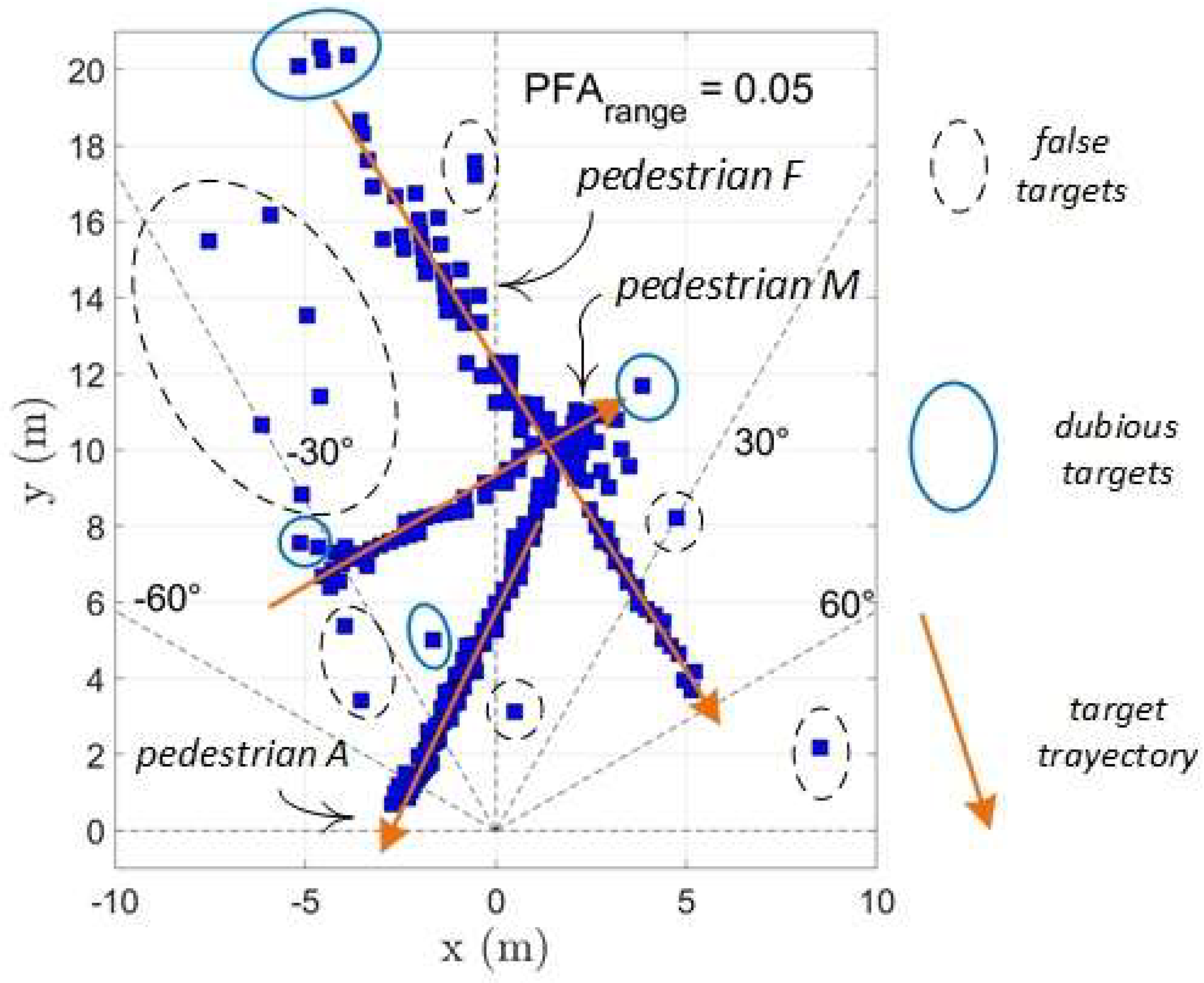
Figure 1 shows the trajectory of the three targets in this first scenario, with all the echoes selected by the analysis program. As stated, the selection of speeds was carried out with a value

P F A_{v e l} = 0.2

, while the result in the figure is the one corresponding to the value

P F A_{r a n g e} = 0.05

. Radar is located at the origin of coordinates.

Figure shows the echoes that most likely belong to one of the targets, located along the path of each pedestrian. There are also false targets, some of them generated by noise peaks or coming from echoes affected by noise, so that their position has been incorrectly estimated. Some of the echoes would fall into the doubtful category, as those framed with a solid blue line, since the observer or a subsequent echo evaluation system could consider as valid, assigning them to a particular pedestrian. It is worth noting that to perform the task of classifying an echo as valid, doubtful or clearly erroneous, it is not enough to observe the final echo map shown in the figure. To make this classification it is necessary to track it in time during the course of the experiment, so that the position of the received echoes can be compared with the real or estimated instantaneous position of each real target.

The second scenario was composed by two pedestrians and a motorbike, describing straight paths and also the return of all three at their initial positions. As in the first case, the raw data obtained from the radar were analyzed again using

P F A_{v e l} = 0.2

, for a first selection of targets, in velocity, and with several values, increasingly small, for the parameter

P F A_{r a n g e}

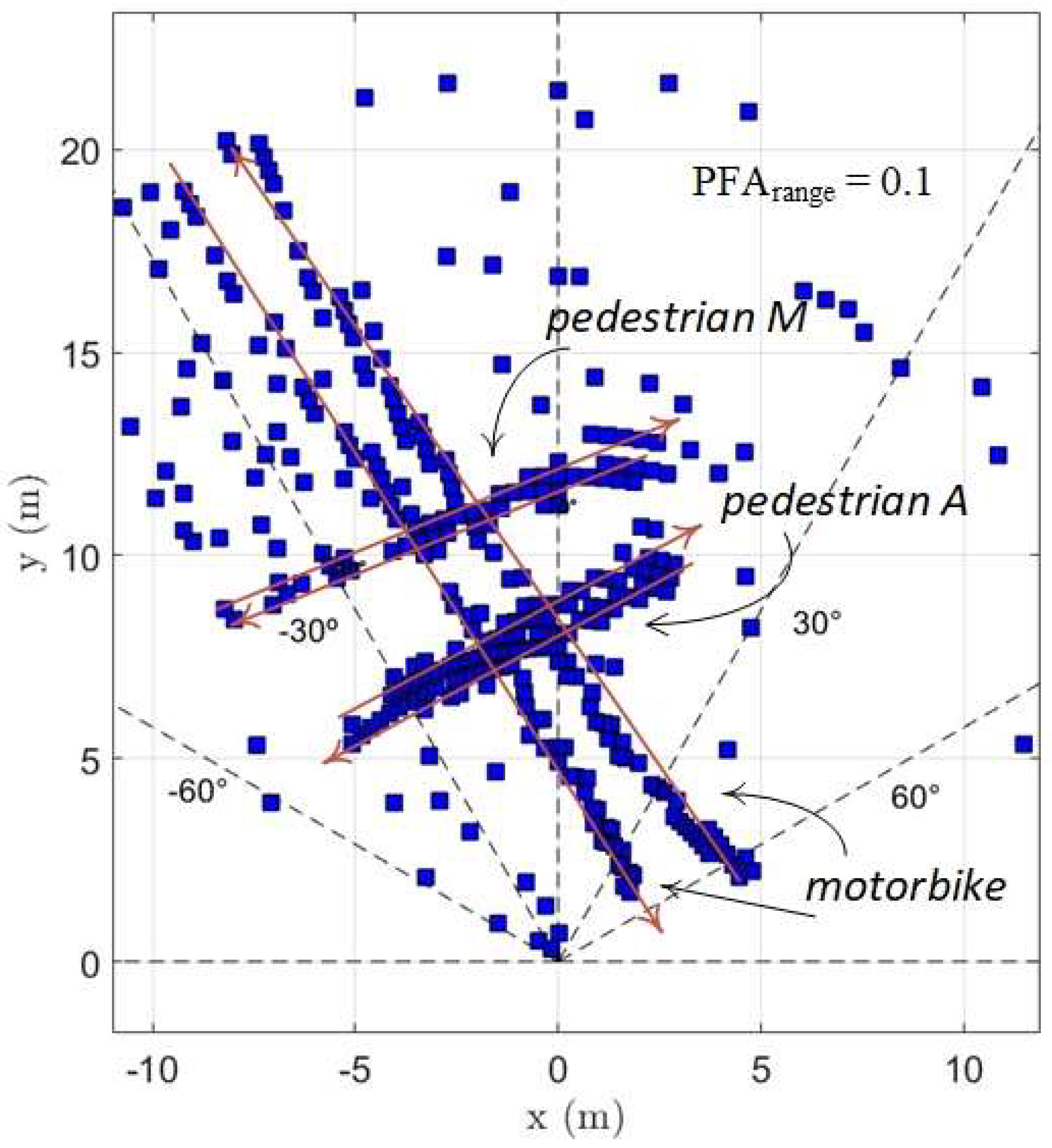
. Figure 2 show the global set of echoes received from the radar during this experiment.

In the particular map of Figure 2 a larger number of echoes, valid and false, can be seen, in comparison with the first scene. This is because a less demanding PFA has been used, but also because the scene duration is longer.

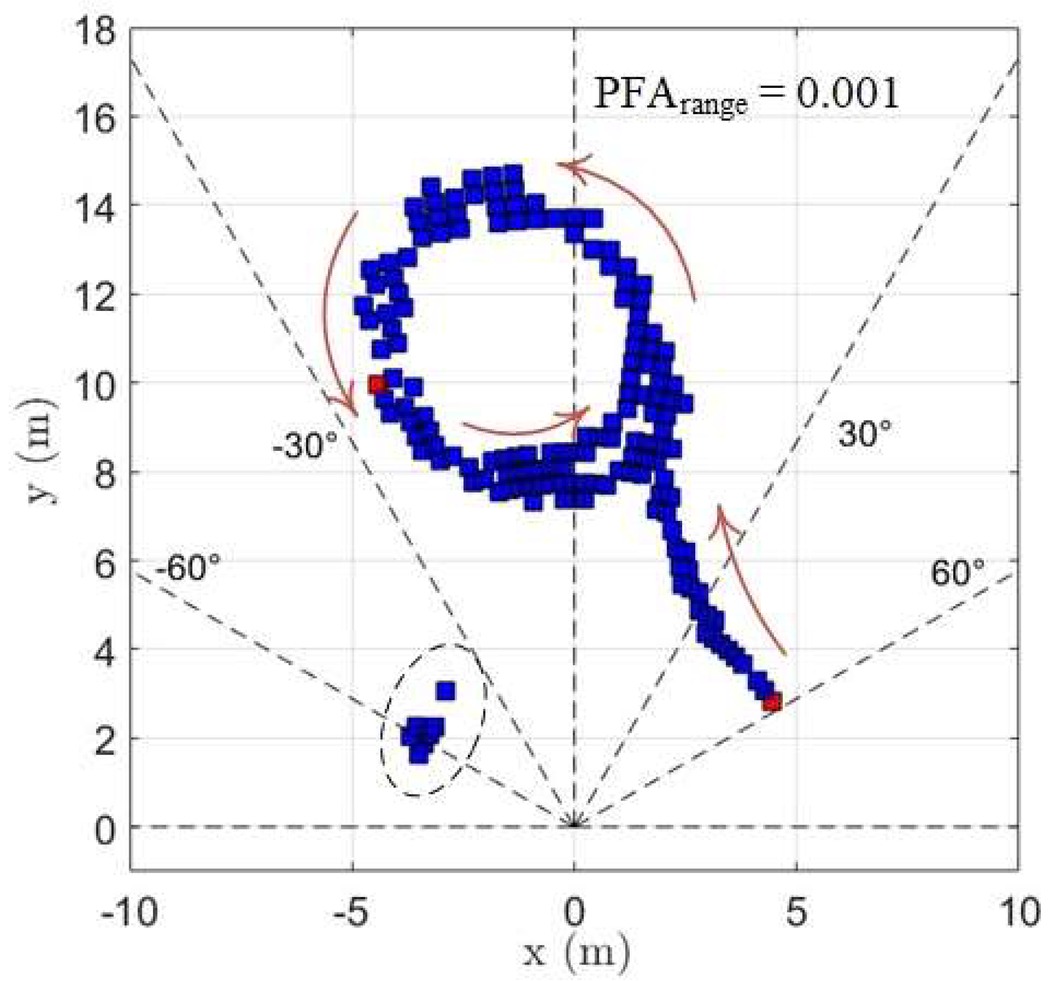
Finally, the third scene is a motorbike describing rounds in front of the radar, with an approximate constant speed. The set of echoes received are shown in Figure 3.

We observed a concentration of false targets near the radar, in a position sixty degrees to the left, as is marked with a dashed contour in the figure. This phenomenon of concentration of echoes where there is not a real object did not happen in the other two experiments, and we do not know why they appear. It could be related with some kind of double reflection of the signal or, perhaps, with the reflection in the wheels, that can introduce an overlap with their own Doppler shift.

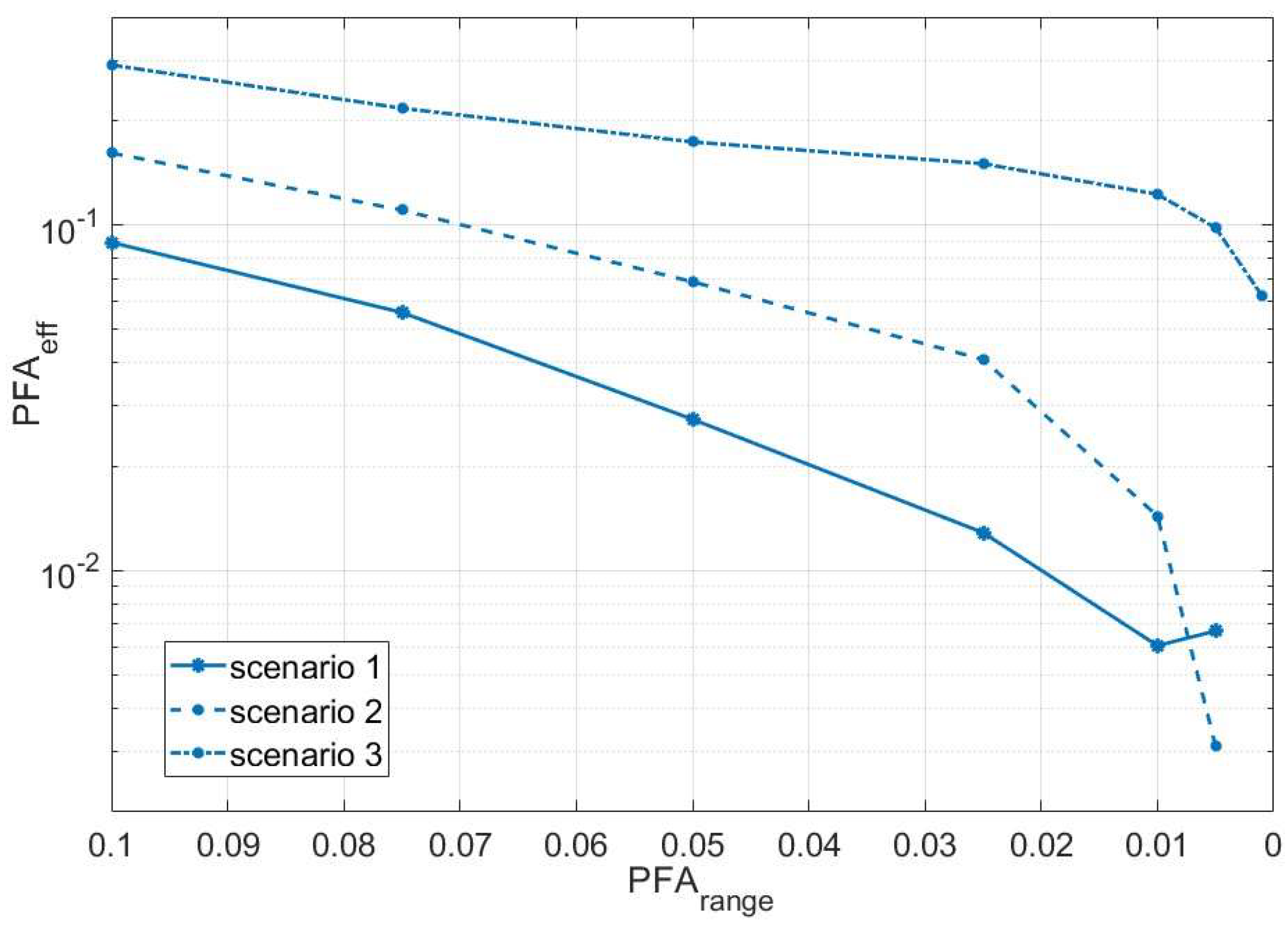
The first analysis carried out in the experiments was to evaluate the number of false targets detected, based on the PFA value used in the detection of targets for each of the selected speeds. That result is shown in Figure 4. It has been defined

P F A_{e f f} = \frac{n º o f f a l s e e c h o e s}{n º o f r e c e i v e d e c h o e s} .

(1)

In this calculation, the class of doubtful echoes has been omitted, assigning them to the set of valid echoes or false echoes in each case.

The choice of a higher or a lower value for the PFA parameter depends on the necessity of having an enough number of echoes: so, in situations where the signal to noise ratio is low, even admitting an important number of false echoes, the choice could be

P F A_{r a n g e} ~ 0.1

. The alternative is minimizing that number of false targets, when the signal to noise ratio is not bad. In this situation a value

P F A_{r a n g e} ~ 0.01

would be more appropriate. In our case, and having enough echoes received per second, avoiding, as much as possible, the number of false echoes seems the best strategy. The behavior of the echoes in the three scenarios is slightly different. In scenarios 1 and 2, the number of false targets is lower than in the other, and with a value of

P F A_{r a n g e} = 0.01

P F A_{r a n g e} = 0.005

, the detection of targets is quite clean. In scenario 3, however, there are a significant larger number of false targets, and a value as low as

P F A_{r a n g e} = 10^{- 3}

should be used to sufficiently filter out false alarms. It must be considered, however, that an unnecessarily small value of this parameter would also cause a significant loss of true echoes. On the other hand, we have fixed most of time the other variable threshold, in the velocity axis, with

P F A_{v e l} = 0.2

, but it must be said that this value could be also relaxed.

3.2. Mean error in range

Each of the pedestrians in the first scene was also followed separately, calculating the average error of the position of the echoes that, with high probability, are coming from the target under study. As explained, the echoes that come from the target (or pedestrian) under test have to be selected manually, and comparing the position of those echoes with the corresponding points on the estimated instantaneous trajectory of each target.

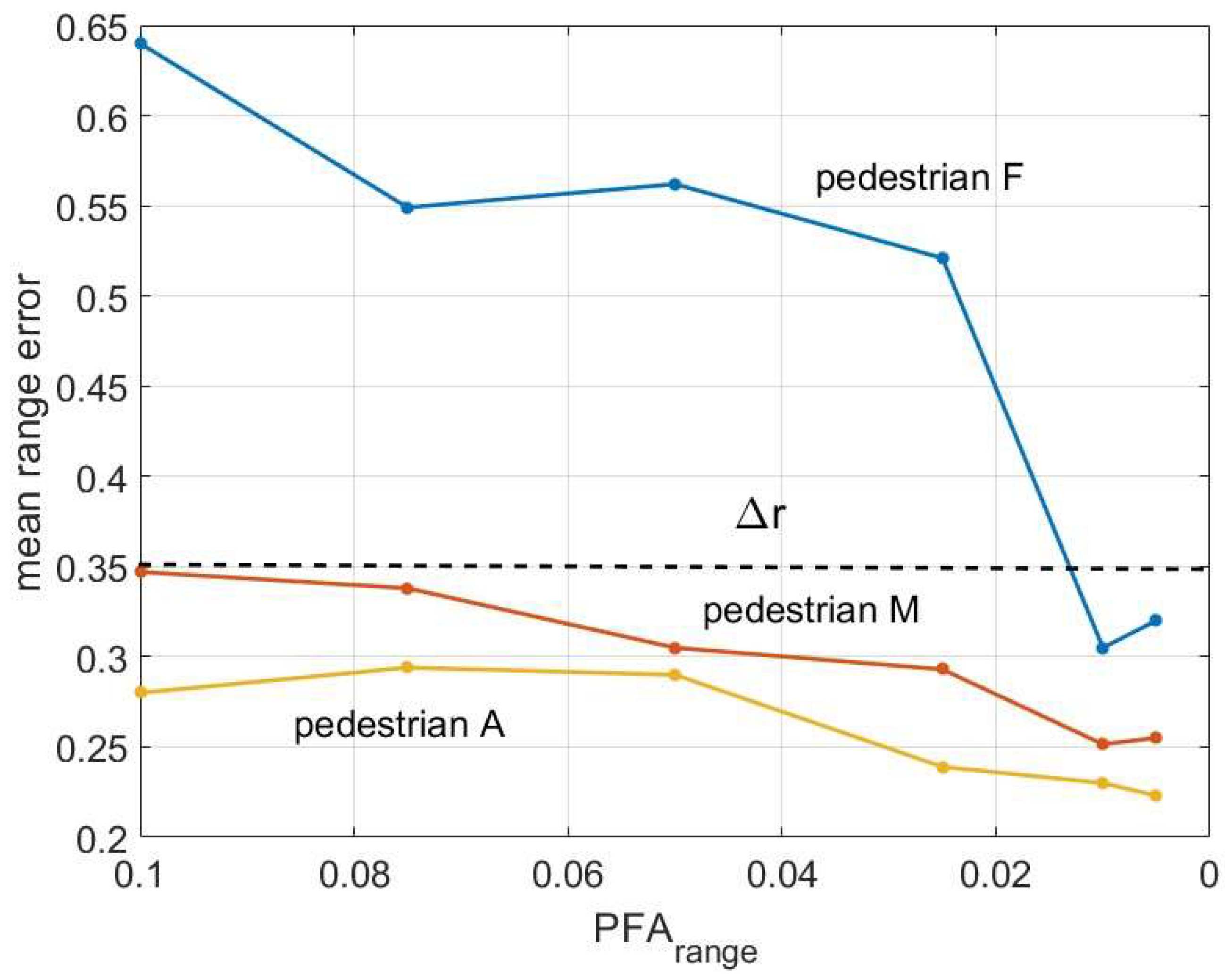
In Figure 5 the obtained mean error in range is shown for the three pedestrians. The basic limit of the system spatial resolution is given by the known expression

∆ r = \frac{c}{2 S T_{c}},

(2)

S being the slope of the frequency temporal variation, c the speed of light and

T_{c}

the duration of a chirp. In our case we have

S = 20 M H z / μ s

and

T_{c} = N_{p c} / f_{s} = 21.33 μ s .

And it results

∆ r = 0.35 m

As it can be seen in Figure 5 the mean error in the localization of the targets does not depend critically of the selected value for the

P F A_{r a n g e}

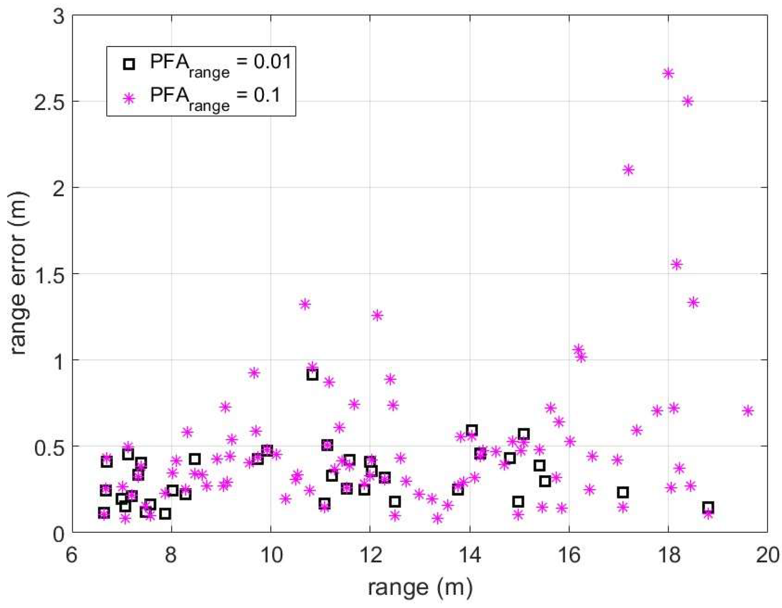
, although is clearly better for low values. This behavior comes from the fact that the targets have been detected correctly most of the time. However, on some occasions, echoes affected by noise or false targets have been considered good. This can be seen in Figure 6, where the error in the localization of one of the pedestrians has been represented as a function of the distance to the radar, and for two cases.

There are two appreciable differences between the two cases shown in the figure. For the higher value of

P F A_{r a n g e}

a quite large number of echoes has been accepted by the system/observer as coming from the target, including some of them with an important error (~2.5m). For the low value of that parameter, however, the number of valid echoes is much lower, as is the maximum error (<1m). It must be remembered, however, that the selection of the 'correct' echoes has been carried out visually, considering what the temporal processing of the signals was showing on the screen. This adds a point of arbitrariness that, on the other hand, cannot be avoided. Nor if the task is performed by an algorithm or an artificial intelligence application, because the system does not know previously the number, nature, trajectory or speed of the targets.

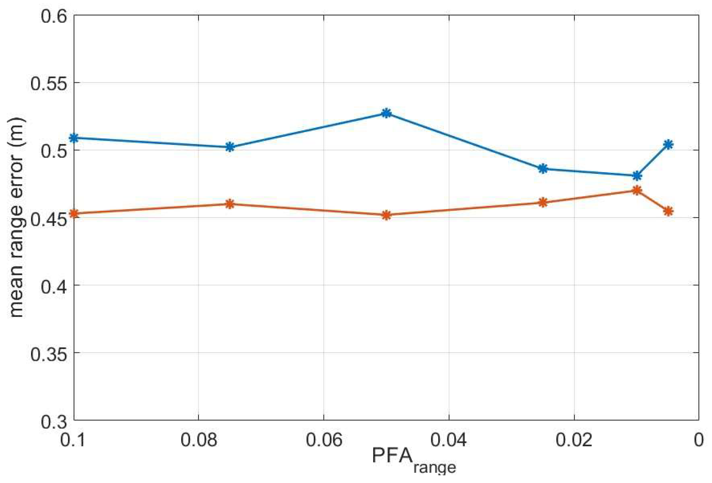
The evaluation of errors has been made also for the two paths of the motorbike in scenario 2, as shown in Figure 7. As the motorbike has an important horizontal dimension, the position mean error is higher than in the case of the pedestrians, although, on the other hand, in this particular experiment the radar never has a complete vision of that horizontal dimension of the vehicle, due to the angle of the paths with respect to the radar position (see Figure 2).

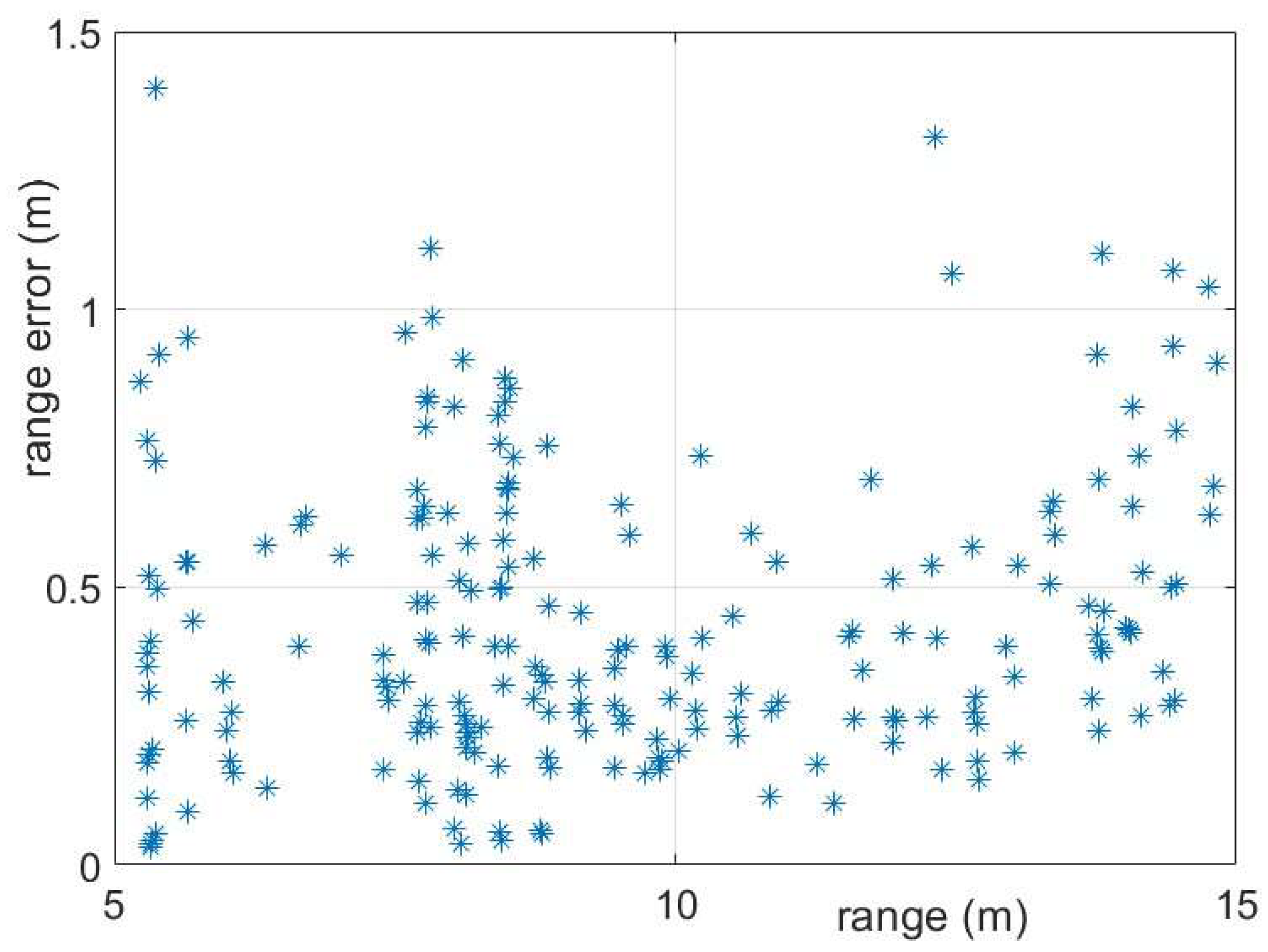
To end this section, in Figure 8 the range error measured during the evolution of the motorbike in scenario 3 is shown. Actually, the trajectory with which the position of the echoes is being compared has been deduced from the echo map itself, averaging the position of echoes as they appear in time, in order to obtain a smooth and continuous path. It could be seen that important errors are reported in some specific positions of the motorbike, which correspond to the moments when the motorcycle is traveling perpendicular to the line of sight of the radar (see Figure 3). As the length of the motorcycle is somewhat more of 2m, the echoes can come from different parts of the vehicle, while the errors are merely calculated with respect to the position of the hypothetical center of the vehicle. Of course, then, errors shown in figure are only a coarse approximation, and most of the echoes come certainly for one or another part of the target.

3.2. Number of echoes per unit of time

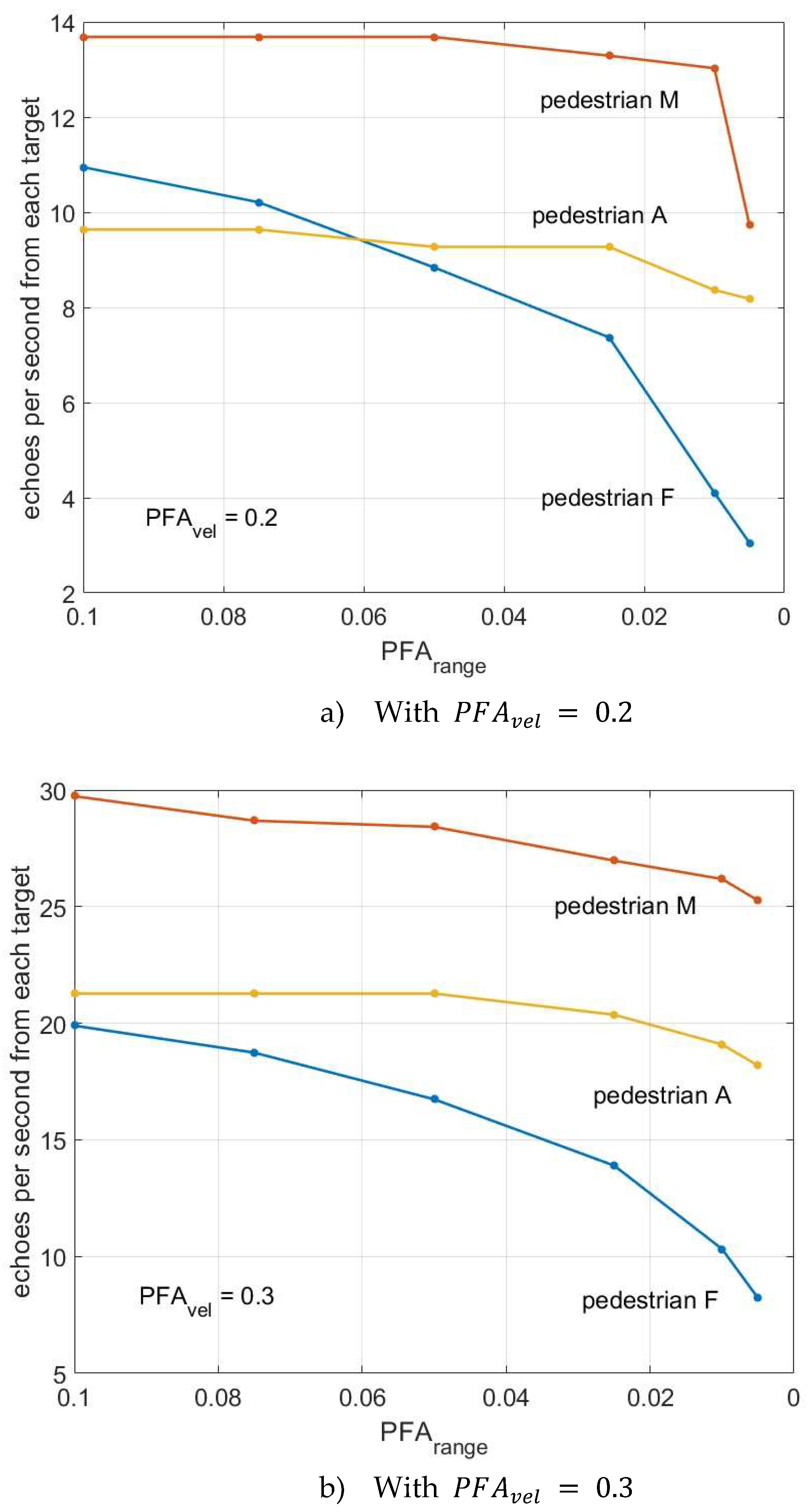
Finally, we have performed a count of the useful echoes available from some of the targets. The most significant point is the number of valid echoes diminishes strongly with a low value of the parameter

P F A_{v e l}

, as can be seen comparing the two plots in Figure 9. If the requirements of the system are about 25 echoes per second (from each target), this parameter,

P F A_{v e l}

, will have to be relaxed consequently. As it has been said before, a too low value of PFAs provokes not only the decrease of false echoes but also of the good ones.

As it can be noted in the figure, the number of good echoes from different targets follows a different behavior. That is due to the different trajectories of the pedestrians. The distance of pedestrian M with respect to the radar has a low variation along time, so that the number of received echoes from her suffers a variation only for the lowest value of PFA. Pedestrian A is progressively approaching the radar, and most of the echoes produced have a very good signal-to-noise ratio. As a consequence, the decreasing of the PFA value has little effect. On the contrary, pedestrian F is in a worst situation to be detected: at the beginning of his path the distance to the radar is larger than for the other two targets, and, at the final state, is near to go out of the field of view of the radar. So, the echoes produced by him are, generally speaking, of lower amplitude. Besides, the echoes of the farthest pedestrian are occasionally intercepted by the other two, when crossing the line of sight of the radar.

Also, worth noting is the fact that an appreciable number of frames sent by the radar have no response at all, or fewer responses than the number of real targets. This is an experimental verification observed in the three scenarios shown in this work.

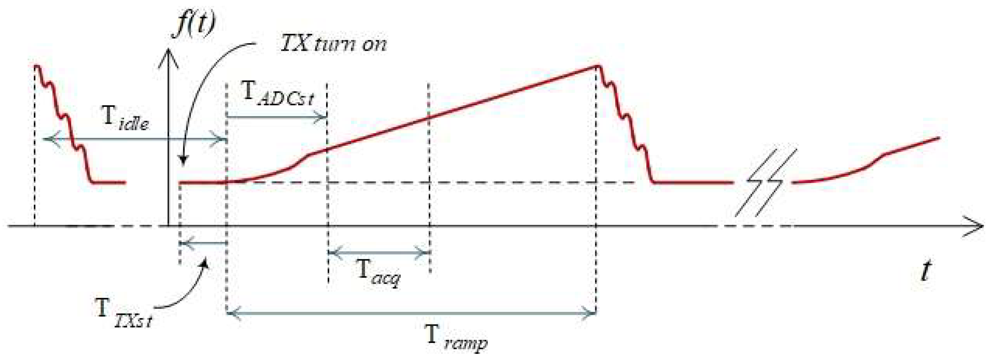
In Figure 10 the time intervals to have into account in the configuration of the TI device are shown [25].

As it was explained above, each chirp was sampled with a frequency

f_{s} = 12 M H z

, up to 256 samples per chirp. So, we have the effective duration of the chirp

T_{a c q} = 256 / 12 M H z = 21.33 μ s .

However the real period of the signal is not related with that value, as seen in the figure. The total period will be

T_{c} = T_{i d l e} + T_{r a m p}

. In our experiments, we took

T_{i d l e} = 100 μ s

and

T_{r a m p} = 60 μ s

, as recommended values. (On the other hand, we set

T_{A D C s t} = 6 μ s

and

T_{T X s t} = 0,

which are the default values in the software pack mmWave Studio, provided by TI). With these values the expected number of frames per second is about 49 frames/s with 128 chirps per frame, and about 24 frames/s with 256 chirps per frame. This numbers include frames without response and frames provoking false echoes. It has to be said, however, that we are not sure if the radar takes some other period of time between frames, and the real expected number of frames emitted per second could be lower than these.

4. Discussion

The main idea of the work was to evaluate the characteristics of the TI AWR1843 radar, in terms of the error committed in distance, the number of false echoes and the number of valid echoes per unit of time. Experiments were done with pedestrians and motorcycles, with the idea that they are the targets that could eventually go unnoticed by the radar.

In the analysis, a double adaptive threshold has been used, one on the speed axis and another on the distance axis, for each speed selected by the first. Both with the CA-CFAR method. The results show that it is a good strategy, and that it provides a level of intuitive control of the number of false echoes.

Initially the experiments were carried out setting the PFA in determining the threshold at speeds with a loose value of 0.2. It was later found that this value actually eliminates too many potentially valid echoes, and a higher value,

P F A_{v e l} = 0.3

, has been found to be more suitable for obtaining a higher echo rate. On the other hand, in our experiments, there is not appreciable difference by using

N c f = 256 o r 128

, so

N c f = 128

is a more economic value.

The maximum error of the radar in estimating the position of a target turns out to be a difficult parameter to quantify, since it depends critically on what criterion is used to assign an echo to a specific target.

The average error has turned out to be very acceptable, taking into account that interpolation techniques can still be included that, in this work, with the exception of zero-padding in the angle-FFT, have not been used.

Finally, we did not set out to estimate the maximum distance at which our radar can capture targets, although, in other measurements not presented in this work, pedestrians have been detected at about 35 meters and a car, in a single attempt, was perfectly detected at 80 meters.

5. Conclusions

We have carried out several experiments with a MIMO radar AWR1863 from Texas Instrument in realistic scenarios with pedestrian and motorcycles, in order to evaluate some critical points of its performance, as the number of false targets, the accuracy in the localization of the targets and the number of valid echoes received per second. These parameters are important for the usefulness of the radar itself and also for the use of the obtained data to make a fusion with the images captured by the cameras in a more complete ADAS system. We use a double CFAR filter, one of them in separating velocities and the other for separate targets in distance. We have used large values in the first of them, with

P F A_{v e l o c i t y} = 0.2 - 0.3

, and more restricted values for the second, with

P F A_{r a n g e}

between 0.1 and 0.001. The results show that it exists a compromise in selecting the value for the two parameters, because a too small number diminish not only the false targets, but also the good ones. The accuracy in range is generally good, although a small value for

P F A_{r a n g e}

helps to avoid disturbance in the measurements due to the false or poorly estimated targets. The mean error along the experiments is about 0.25 m for pedestrians and 0.5 m for the motorbike. The maximum error in the localization of targets cannot be estimated properly, because it is not possible to discriminate between false targets and positions erroneously calculated due to the present noise. Moreover, assigning a singular echo to a particular target depends on some chosen criterion, probably in a further stage in the complete detection algorithm, but always with a certain degree of arbitrariness.

Author Contributions

Conceptualization, F. Dios, J.A Lázaro and A. Lerín; methodology: F. Dios, J.R. Casas; experimental work: S. Torres-Benito, F. Dios and J.A. Lázaro; software: F. Dios and S. Torres-Benito; validation: J.R. Casas, Jorge Pinazo and A. Lerín; writing—original draft preparation: F. Dios, S. Torres-Benito and J.A. Lázaro; funding acquisition, J.A Lázaro and A. Lerín. All authors have read and agreed to the published version of the manuscript.

Funding

This research was funded by Capgemini as part of the project “Percepción Inteligente para los Vehículos Autónomos y Conectados” (InPercept) financed by “Centro para el Desarrollo Tecnológico Industrial” (CDTI), Spanish “Ministerio de Ciencia e Innovación”, under grant number PTAS-20211011, co-founded by European Union, NextGenerationEU, “Plan de Recuperación, Transformación y Resiliencia”.

Conflicts of Interest

The authors declare no conflict of interest.

References

I. Bilik, O. Longman, S. Villeval and J. Tabrikian, "The Rise of Radar for Autonomous Vehicles: Signal Processing Solutions and Future Research Directions," IEEE Signal Processing Magazine, vol. 36, n. 5, pp. 20-31, Sept. 2019. [CrossRef]
H.A. Ignatious, H. El-Sayed, M. Khan, “An overview of sensors in Autonomous Vehicles,” Procedia Computer Science, vol. 198, pp. 736-741, 2022. [CrossRef]
X. Gao, S. Roy and G. Xing, "MIMO-SAR: A Hierarchical High-Resolution Imaging Algorithm for mmWave FMCW Radar in Autonomous Driving,” IEEE Transactions on Vehicular Technology, vol. 70, n. 8, pp. 7322-7334, 2021. [CrossRef]
E. Marti, J. Perez, M.A. de Miguel M.A., F. Garcia, “A review of sensor technologies for perception in automated driving,” IEEE Intelligent Transportation Systems Magazine, vol. 11, n. 4, pp. 94-108, 2019. [CrossRef]
G. Reina, D. Johnson, and J. Underwood, “Radar sensing for intelligent vehicles in urban environments,” Sensors, vol. 15, n. 6, pp. 14661–14678, 2015. [CrossRef]
S. M. Patole, M. Torlak, D. Wang and M. Ali, "Automotive radars: A review of signal processing techniques,” IEEE Signal Processing Magazine, vol. 34, n. 2, pp. 22-35, 2017. [CrossRef]
M. Wagner, F. Sulejmani, A. Melzer, P. Meissner and M. Huemer, "Threshold-Free Interference Cancellation Method for Automotive FMCW Radar Systems,” 2018 IEEE International Symposium on Circuits and Systems (ISCAS), Florence, Italy, 2018, pp. 1-4. [CrossRef]
W. Stark, M. Ali, M. Maher, “Digital Code Modulation (DCM) for Automotive Application,” Uhnder White Paper, 2020.
R. Plšičík, M. Danko, “Introducing to using mmWave Radar development board AWR1843,” IEEE ELEKTRO Conference, Krakow, 2022. [CrossRef]
Y. Peng, X. H. Wang, J. J. Hu, Y. Xu and X. W. Shi, "Design of Miniature Millimeter Wave Radar System Based on TI Integrated Chip,” 2022 International Conference on Microwave and Millimeter Wave Technology (ICMMT), Harbin, China, 2022, pp. 1-3. [CrossRef]
X. Gao, G. Xing, S. Roy and H. Liu, "Experiments with mmWave Automotive Radar Test-bed,” 2019 53rd Asilomar Conference on Signals, Systems, and Computers, Pacific Grove, CA, USA, 2019, pp. 1-6. [CrossRef]
X. Gao, S. Roy, G. Xing and S. Jin, "Perception Through 2D-MIMO FMCW Automotive Radar Under Adverse Weather," 2021 IEEE International Conference on Autonomous Systems (ICAS), Montreal, QC, Canada, 2021, pp. 1-5. [CrossRef]
A. Correas-Serrano, M.A. González-Hiuci, “Experimental evaluation of compressive sensing for DoA estimation in automotive radar,” 19^th International Radar Symposium IRS, Bonn, 2018. [CrossRef]
S. Patole, A. B. Baral and M. Torlak, "Fast 3D Joint Superresolution Algorithm for Millimeter Wave FMCW Radars,” IEEE Open Journal of Signal Processing, vol. 4, pp. 346-365, 2023. [CrossRef]
Y. Huang, H. Zhang, K. Guo, J. Li, G. Xu and Z. Chen, "Density-Based Vehicle Detection Approach for Automotive Millimeter-Wave Radar," 2020 IEEE 3rd International Conference on Electronic Information and Communication Technology (ICEICT), Shenzhen, China, 2020, pp. 534-537. [CrossRef]
A. Pirkani, S. Cassidy, S. Pooni, M. Cherniakov and M. Gashinova, "Modelling and experimental validation of radar - environment interaction in automotive scenarios,” International Conference on Radar Systems (RADAR 2022), Hybrid Conference, Edinburgh, UK, 2022, pp. 395-400. [CrossRef]
F. Meinl, M. Stolz, M. Kunert and H. Blume, "An experimental high-performance radar system for highly automated driving," 2017 IEEE MTT-S International Conference on Microwaves for Intelligent Mobility (ICMIM), Nagoya, Japan, 2017, pp. 71-74. [CrossRef]
Y. Golovachev, A. Etinger, G.A. Pinhasi, Y. Pinhasi, “Millimeter Wave High Resolution Radar Accuracy in Fog Conditions—Theory and Experimental Verification”. Sensors 2018, 18, 2148. [CrossRef]
A. Rasouli and J. K. Tsotsos, "Autonomous Vehicles That Interact with Pedestrians: A Survey of Theory and Practice,” IEEE Transactions on Intelligent Transportation Systems, vol. 21, n. 3, pp. 900-918, 2020. [CrossRef]
P. Nimac, A. Krpič, B. Batagelj, A. Gams, “Pedestrian Traffic Light Control with Crosswalk FMCW Radar and Group Tracking Algorithm,” Sensors 2022, vol. 22, pp. 1754. [CrossRef]
S. Sun, A.P. Petropolu, H.V. Poor, “MIMO radar for Advanced Driver-Assistance Systems and autonomous driving,” vol. 37, n.4, pp. 98-117, IEEE Signal Processing Magazine 2020. [CrossRef]
C. Iovescu, S. Rao, “The fundamentals of millimeter wave sensors,” TI report SPYY005, 2017.
S. Rao, “MIMO Radar,” TI Application Report SWRA554A, May 2017, revised July 2018.
O. Faus, “Signal Processing for mmWave MIMO Radar,” Master Thesis, University of Gävle, Gävle, 2015.
“Programming Chirp Parameters in TI Radar Devices,” Application Report SWRA553A–May 2017 – Revised February 2020.
N. Levanon, Radar, Editor: Robert A. Meyers, Encyclopedia of Physical Science and Technology (Third Edition), Academic Press, 2003, pp. 497-510.
C. Katzlberger, “Object detection with automotive radar sensors using CFAR algorithms,” Bachelor Thesis, Johannes Kepler University, Lenz, 2018.
S. Ren, S. Han and B. Wang, "Stationary and Small Target Detection for Millimeter-Wave Radar," 2022 IEEE 22nd International Conference on Communication Technology (ICCT), Nanjing, China, 2022, pp. 1698-1702. [CrossRef]
C. Xu, F. Wang, Y. Zhang, L. Xu, M. Ai and G. Yan, "Two-level CFAR Algorithm for Target Detection in mmWave Radar," 2021 International Conference on Computer Engineering and Application (ICCEA), Kunming, China, 2021, pp. 240-243. [CrossRef]
S. Wang and R. Herschel, "Fast 3D-CFAR for Drone Detection with MIMO Radars," 2021 18th European Radar Conference (EuRAD), London, United Kingdom, 2022, pp. 209-212. [CrossRef]

Figure 1. Global map of the received echoes along the time in scenario 1, while three pedestrians are walking along straight paths.

Figure 2. Echoes received over time in the second experiment, with two pedestrians going and coming along approximately the same path, and a motorcycle, describing the longest and most vertical paths.

Figure 3. The graph shows a motorcycle occupying the center of the scene and doing some laps in front of the radar at an approximately constant speed.

Figure 4. Effective probability of false alarm in the three scenes, obtained as a function of the PFA parameter chosen for the detection of targets in distance. For the selection of velocities, the value

P F A_{v e l} = 0.2

was used in all cases.

P F A_{v e l} = 0.2

was used in all cases.

Figure 5. Mean error in distance obtained for individual targets in the first scenario.

Figure 6. Range error committed along the tracking of one of the targets in scenario 1, for two values of the

P F A_{r a n g e}

parameter.

Figure 6. Range error committed along the tracking of one of the targets in scenario 1, for two values of the

P F A_{r a n g e}

parameter.

Figure 7. Mean range error obtained in the localization of the motorbike in scenario 2 along the two different paths.

Figure 8. Estimated range error of the motorcycle in scenario 3, as a function of the distance to the radar, with

P F A_{r a n g e} = 0.001

Figure 8. Estimated range error of the motorcycle in scenario 3, as a function of the distance to the radar, with

P F A_{r a n g e} = 0.001

Figure 9. Number of valid echoes per second from each target in scene 1.

Figure 10. Signal time parameters in the radar configuration.

Disclaimer/Publisher’s Note: The statements, opinions and data contained in all publications are solely those of the individual author(s) and contributor(s) and not of MDPI and/or the editor(s). MDPI and/or the editor(s) disclaim responsibility for any injury to people or property resulting from any ideas, methods, instructions or products referred to in the content.

© 2024 by the authors. Licensee MDPI, Basel, Switzerland. This article is an open access article distributed under the terms and conditions of the Creative Commons Attribution (CC BY) license (http://creativecommons.org/licenses/by/4.0/).

Copyright: This open access article is published under a Creative Commons CC BY 4.0 license, which permit the free download, distribution, and reuse, provided that the author and preprint are cited in any reuse.