1. Introduction
Drones are small unmanned aerial vehicles (UAVs) that have become popular, among other things, due to their adaptation for recreational use, environmental monitoring, surveillance, security, commercial use, etc. Although their use can have undoubted advantages, there has also been an increase in the use of drones for illegal activities. Some examples of these illicit acts are detailed in [
1], including their use in airports and rescue operations, where they could disrupt operations and cause possible collisions between planes, helicopters and drones. There have also been reports of drones being used for smuggling in prisons, as penetration nodes in cyber-attacks to access WiFi networks in offices, and in residences and patrols, where they are used as spy cameras. The development of technologies to detect drones as a means to control these illegal practices, or to manage the movement of drones in cases of legal use, is necessary.
Several techniques for drone detection can be found in the literature. Technologies based on optical sensors, radio frequency, radar and acoustic sensors are compared in [
2], detailing their advantages and disadvantages. A comprehensive description of these techniques is also given in [
3]. It is pointed out that visual inspection techniques with cameras require a clear line of sight, which is not possible in rainy, foggy scenarios, or in the presence of occlusions. The cameras used can work in the visible spectrum, or in the infrared spectrum, but in the latter case the cost is higher. Nevertheless, detection based on images obtained with cameras can exploit powerfull image processing and classification algorithms, such as YOLO (You Only Look Once) [
4].
Detection of the radio frequency signal emitted in the drone’s communication with the controller offers good performance, but is not possible with autonomous UAVs. Radar sensors are effective but expensive and have limitations for detecting static or low-speed drones, due to the application of digital signal processing techniques for clutter cancellation. A comprehensive review of the state of the art in the above techniques is beyond the scope of this paper, which focuses on acoustic detection as an alternative.
Acoustic detection avoids some of the problems of the other sensors: it does not require line of sight between the sensor and the drone, it can be carried out in low visibility situations (such as at night or in foggy situations), and in the presence of obstacles, for example, in forested surroundings. However, the detection range is assumed a priori to be low, caused by sound attenuation with distance, by the sensitivity of the sensors, and by the presence of ambient noise, which is difficult to avoid. Preliminary studies, such as the one presented in [
6], suggest that acoustic detection of UAVs is cost-effective and presents itself as an efficient and economical alternative. Detection is favored because the rotation of a drone’s blades generates a characteristic acoustic footprint, which makes it possible to distinguish the sound generated by the drone from other sound sources, even if the signal-to-noise ratio is low.
There are numerous works in the literature about acoustic detection of UAVs. For example, in [
7] a real-time system using a single microphone for drone detection and monitoring is presented, based solely on the spectral analysis of the input signal. In [
9] the authors present a method that calculates the spectrogram of the received signal to find robust points in the time-frequency domain and thus use the fingerprinting technique for feature extraction.
However, currently, most of the work on acoustic detection of UAVs uses some form of machine learning method, with a clear trend towards research in deep learning models.
In the field of machine learning, innovative approaches have been proposed for UAV detection. In [
10], a drone detection system using multiple acoustic nodes and machine learning models is presented. This system uses an empirically optimised configuration of nodes, enabling them to detect drones in protected areas. Another example of the use of machine learning algorithms is illustrated in [
11], which explores various short-term parameterizations in the time-frequency domain of ambient audio data. The extracted parameters are used to feed an unmanned aerial vehicle warning system, which employs support vector machines (SVMs) to recognize the sound fingerprint of drones, leading to effective preliminary results.
The efficacy of deep learning algorithms with metrics such as accuracy, F1 score, precision, and recall, has been assessed in [
12]. In [
13], a CNN is proposed to which features extracted by STFT preprocessing of the drone acoustic signal are applied. Acoustic signals from motorcycles and scooters were also employed in the experiments, as they have similar harmonic characteristics to the drone signal. The performance of the model was evaluated as a function of the number of training epochs. This approach achieved a detection rate of 98.97% with a false alarm rate of 1.28% for a 100 epoch model. Furthermore, an approach to drone detection using deep learning which combines Mel-frequency cepstral coefficients (MFCCs) and Log-Mel spectrogram features extracted from the sound signal, is proposed in [
14]. Additionally, [
15] investigates the use of Recurrent Neural Networks (RNN) in real-time UAV sound recognition systems, specifically employing Mel-spectrograms with Kapre layers. Another interesting paper recently available is [
16], where authors combine time and frequency domains features to improve the accuracy of drone detection systems based on deep learning, obtaining an accuracy of 0.98 in the best case.
The main difficulty for the development of drone or UAV detection systems with deep learning techniques lies in the availability of useful data for training. Strategies to overcome this problem include the use of
data augmentation or
transfer learning. In [
17], pre-trained CNN fitting is explored using a custom acoustic dataset to classify sounds and detect drone-specific features. The obtained results show an average accuracy of 0.88. On the other hand, in [
18], a performance comparison between a CNN network, RNN networks and Convolutional Recurrent Neural Networks (CRNNs) is carried out. The results reveal superior performance for the convolutional network in accurately detecting drones from acoustic signals. These studies highlight the potential of transfer learning in improving audio-based drone detection systems.
Finally, it is worth mentioning the comprehensive review presented in [
19] on detection and classification methods up to the time of publication, covering various modalities, including detection by acoustic signals, which remains an emerging area of research. The study highlights the difficulty of benchmarking due to variations in drones, ranges, characteristics, classification methods and performance metrics used by different authors. However, it highlights the lack of in-depth research on the impact of range on detection effectiveness. A more recent review paper of UAV detection techniques is [
20], which reviews the knowledge about drone detection, studing the threats and challenges faced due to drones’ dynamic behavior, size and speed diversity, battery life, etc. Novel processing techniques to improve the accuracy and efficiency of UAV detection and identification are also studied.
Considering the lack of studies on the influence of the distance between the drone and the sensor system on the detection capability, this paper focuses on evaluating the performance of different machine learning algorithms (including deep learning) to detect drones at different distance ranges using the sound emitted, in order to determine the maximum distance at which it is possible to detect drones with acoustic systems. A comparison between different detection methods is carried out, considering both simple machine learning algorithms and sophisticated methods based on deep learning with transfer learning, thus representing the most prevalent approaches in the literature. With this in mind, several machine learning methods have been compared, such as linear discriminant analysis, multilayer perceptron, support vector machine, random forest, and YAMNet as an example of a deep learning system which exploits transfer learning. The study, in addition to assessing the feasibility of drone detection as a function of distance, considers the detection of drones against others sound sources with comparable spectral characteristics.
The paper is organised as follows. After this introductory section,
Section 2 presents the main characteristics of the signals emitted by the drones, which will be taken into account in the design of the sound detection system.
Section 3 describes the machine learning based detectors tested in this work.
Section 4 includes the description of the sound database used in the training and testing of the detection systems, the features calculated from the signal, and some training and testing details. The results obtained, are presented and discussed in
Section 5, and the main conclusions drawn from this study are presented in
Section 6.
2. Signal characterization
The sound of a drone is mainly generated by the motors and blades that propel it. The signal is typically non-stationary, since the rotation of these components generates a stationary harmonic sound only if the speed is constant. But during flight in different directions, the blades must rotate at varying speeds, and in the case of drones with multiple rotors, each one may rotate at a different speed, generating sounds with unrelated fundamental frequencies and creating a non-periodic signal.
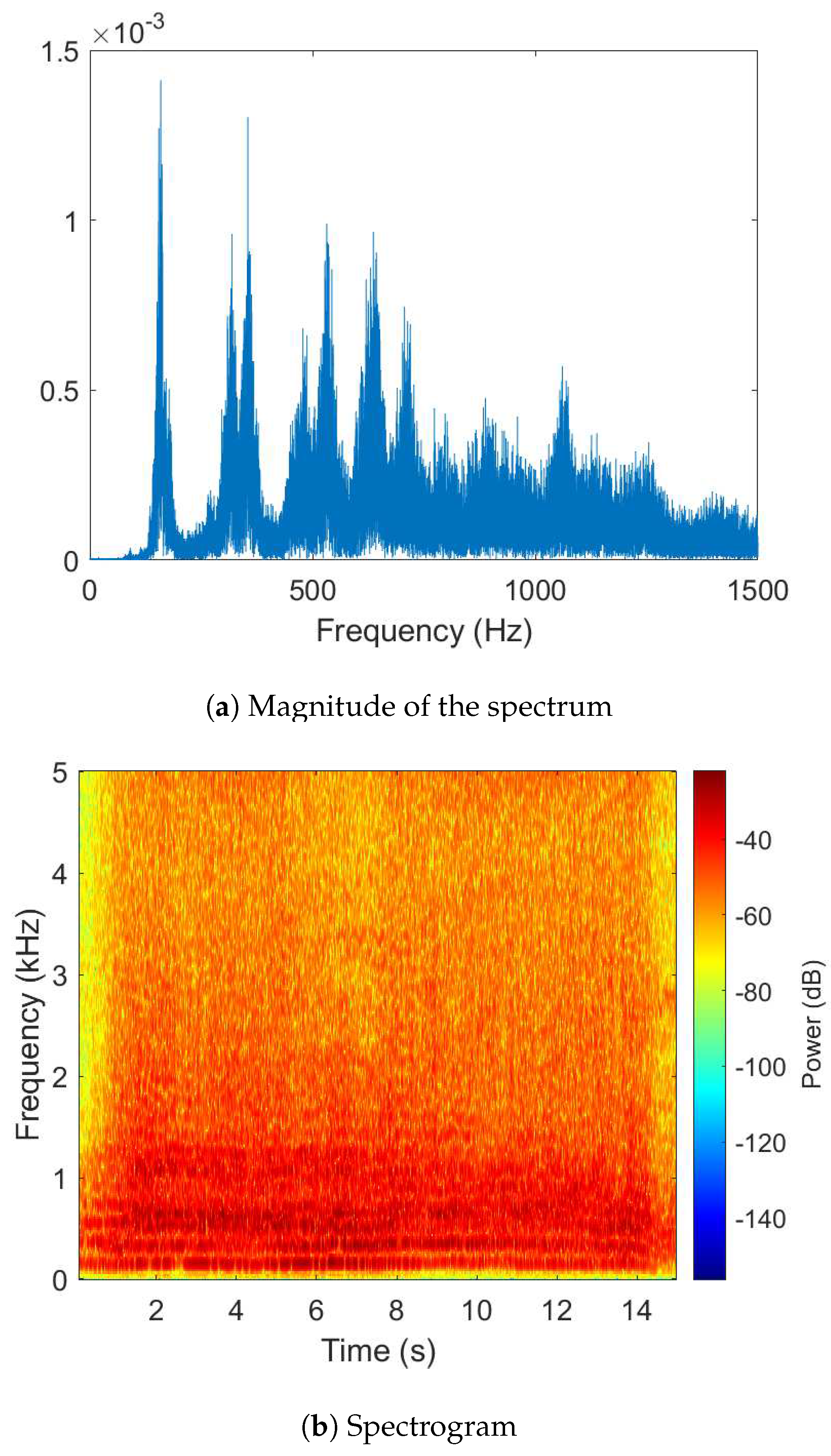
The variations in the energy distribution of the received signal can be best studied in the frequency domain, where different patterns are observed that can be useful for UAV detection. On the one hand, energy is concentrated in characteristic frequency bands associated with average rotational speeds for lift and motion. In addition, most of the energy resides in low frequency bands. On the other hand, the envelope of the spectrum has peaks and valleys, resulting from the combined signals of the engines and blades. These peaks and valleys are approximately equidistant and the frequencies at which they occur vary slowly in practice. These frequencies and the shape of the spectrum envelope are related to the type of UAV, providing valuable information for detection, classification and identification purposes. These features are evident in
Figure 1a, which illustrates the frequency analysis of a Hobbyking FPV250 drone as an example.
In particular, there is a low frequency band where most of the energy of the spectrum is concentrated and from this band quasi-horizontal lines called HElicopter Rotor Modulation (HERM) are born. These lines appear when a time-frequency analysis is performed with the Short-time Fourier transform, using a window length large enough to cover several rotation cycles of the drone’s propellers. An example of these lines can be seen in the spectrogram in
Figure 1b. This low frequency information could be critical in distinguishing drones from other devices, especially since low-frequency sounds are less attenuated than high-frequency sounds when they propagate through the air, making the detection at long distances easier.
3. Detection System Based on Machine Learning
This paper studies learning machine drones detection capability as a function of distance. As a novel aspect in comparison with other papers in which the performance of the detector is measured with parameters such as Accuracy, Precision, Recall, or F1, detection is studied from the point of view of the Neyman-Pearson criterion [
21]. This detector maximizes the probability of detection (
), for a fixed probability of false alarm (
), and it is especially useful in binary hypothesis testing when the assignment of costs and the knowledge of a priori probabilities are difficult.
The possibility of approximating the Neyman-Pearson detector with learning machines has been previously demonstrated, when the mean squared error [
22] or the cross-entropy error [
23] are used as error function for training. The Neyman-Pearson detector can also be approximated with appropriately trained SVMs [
24]. In this paper, machine learning-based detectors that approximate the Neyman-Pearson detector are trained and then tested by comparing their output to a threshold. The variation of the threshold allows to vary the value of
, and for each estimated value, the corresponding
is estimated. The representation of
versus
is the ROC (Receiver Operating Characteristic) curve, which allows to evaluate the quality of the detector.
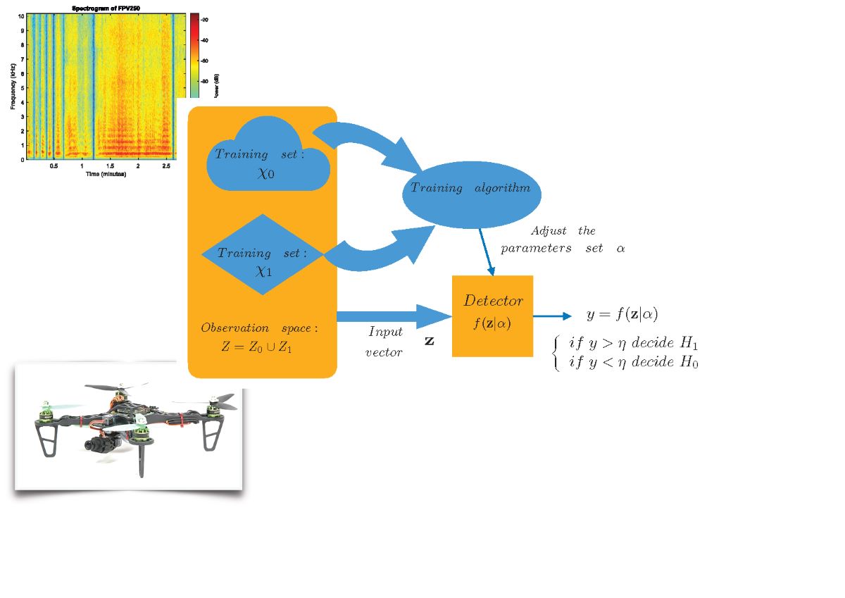
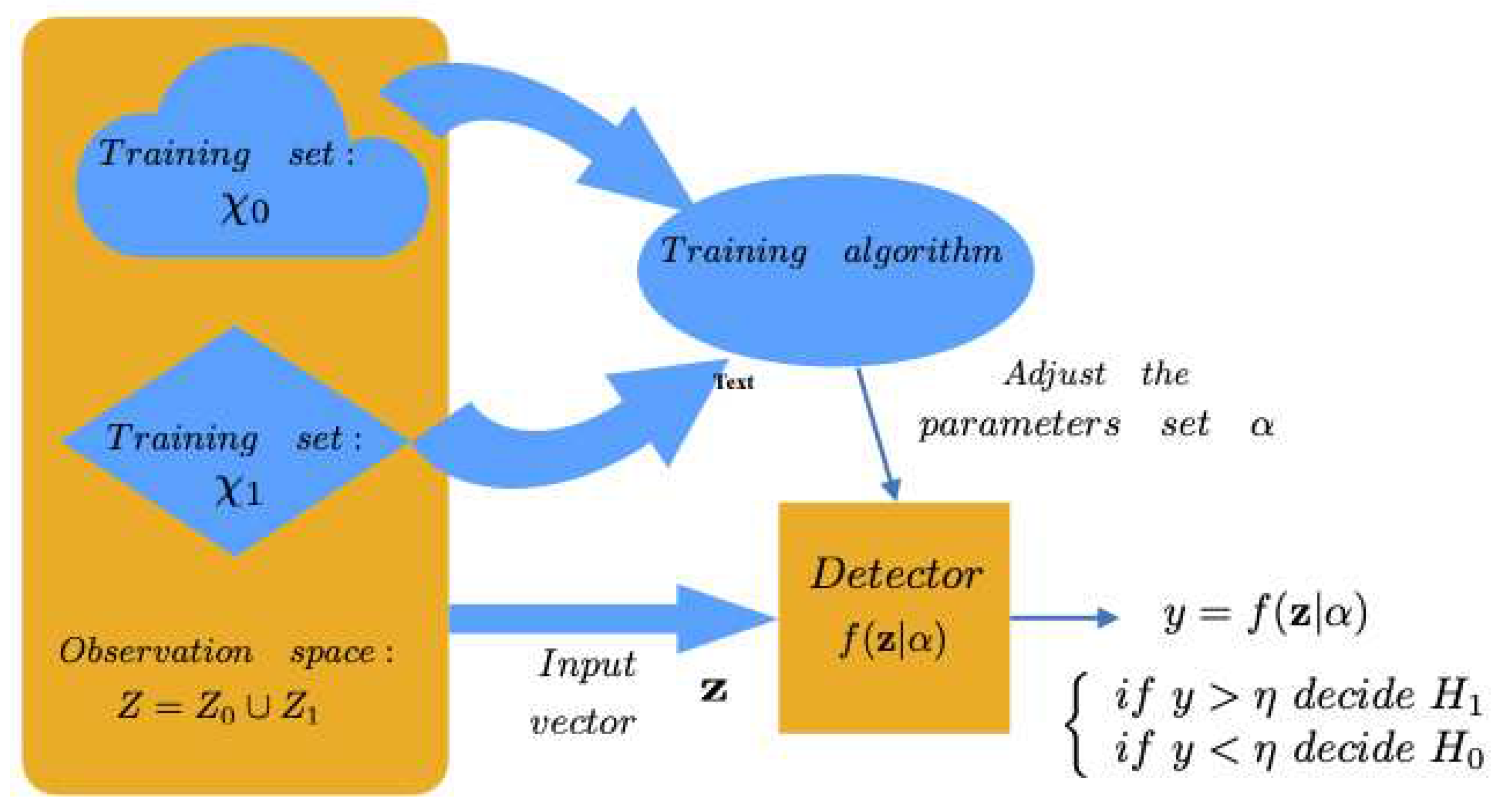
A learning machine is considered with only one output to classify input vectors into two hypothesis or classes, and , representing the absence of drones and the presence of drones, respectively. The set of all possible input vectors generated under hypothesis is , with probability density function , and the ensemble of all possible input vectors is . A trainins set , with elements of each class ( is available. This trainins set is labeled, with desired or target outputs . The vector contains the desired outputs of the patters applied to the classifier. The oputput of the learning machine is for the input vector , representing the set of paramiters fitted during training.
Figure 2.
Structure of the learning-machine based detector.
Figure 2.
Structure of the learning-machine based detector.
To evaluate the variation of the drone detection probability as a function of the distance between the drone and the system, learning machine based detectors have been implemented to approximate the optimal Neyman-Pearson detector, and tested with attenuated audio signals with a frequency and distance dependent function. The learning machines used to develop these detectors are the following:
- 1.
Least squares lineal classifier. Linear discriminant (LD) is a supervised classification method based on computing a linear combination of various features in order to differentiate between two specific classes. In the process, the least squares classifier projects the data into a lower dimensional space, pursuing the objective of maximizing the separation between classes and facilitating the classification task. The vector of outputs of the linear discriminat for the set of features vectors in the test set, is calculated with the following expression:
where
is a
vector with the weights of the linear discriminant (including the bias),
t is a
vector containing the target values (+1 and -1) of the P design patterns and
is a
matrix containing a row of ones for the bias and the L features of the P design patterns. The weights vector is calculated after least-squares minimization, with expression (
2), where
is a vector with the desired outputs for the training data, and
is a matrix containing the training patterns:
- 2.
-
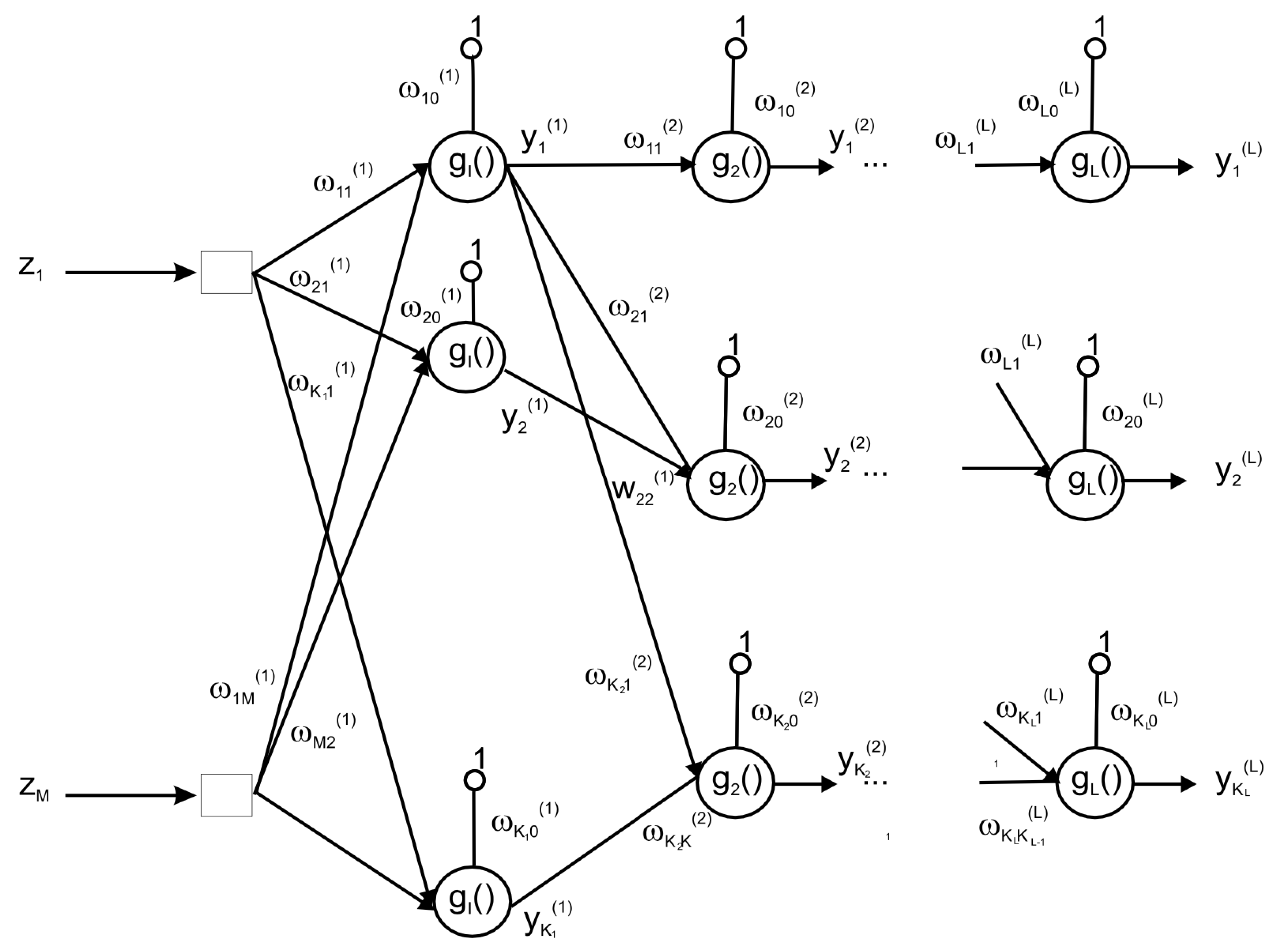
Multilayer perceptron (MLP). The MLP is an artificial neural network that has the ability to identify complex patterns in data by adjusting the connection weights between neurons during the training process. The operation of MLP involves applying a processing step to an input vector
, during which it is multiplied by weight vectors to obtain the input to the activation function of neurons in the hidden layers,
. The outputs of these hidden neurons are also processed in a similar manner, and finally the desired output is obtained.
Figure 3.
Multilayer perceptron structure.
Figure 3.
Multilayer perceptron structure.
In this paper, we have chosen to use a perceptron with a single hidden layer, since it can approximate any discriminant function if a sufficient number of neurons in that hidden layer are used. The neurons in this layer are connected to the output, and this output is compared with a predefined threshold to make decisions in the detection and classification process. We have used the Quasi-Newton-based backpropagation training algorithm, where the connection weights are adjusted at each iteration or epoch in batch mode, i.e., using subsets of training data instead of the full set. This not only reduces the computational burden, but also significantly speeds up the training process.
- 3.
-
Support Vector Machine (SVM). The SVM method operates by transforming the input vectors into a higher dimensional space, where they can be clearly separated using a hyperplane that divides the two classes. This method can be understood as a two-layer neural network: the first layer uses a kernel function, typically a radial basis function (RBF), while the second layer employs a linear basis. This combination results in a model capable of handling complex, high-dimensional data, even those that do not follow linear patterns.
Therefore, the function implemented by the SVM is a linear function of the results of mapping the input pattern
into a higher dimensional space
with the kernel functions
, being
M the dimension of the new space. The parameters of the SVM are the weights vector
, the bias constant, and the parameters the functions
depend on. The output of the SVM is obtained as follows, where
is a vector with the outputs of the kernel functions:
Before processing the data with this method, a normalization has been applied to ensure that all data have the same scale. This technique is essential as it ensures an accurate fit of the model to the data and prevents certain characteristics from having a disproportionate weight in the decision-making process.
To implement the approximation to the Neyman-Pearson detector, the 2C-SVM must be used [
24]. Its training consist in solving the following optimization problem with constraints:
subject to:
This optimization is equivalent to minimizing the following objective function [
24]:
where parameters
and
C are used to control the costs associated to the errors in classifying patters of each hypothesis,
is the desired output for pattern
, and
is the Heaviside step function. After training, the weigths vector and the parameters of the kernel functions are obtained.
- 4.
-
Random Forest.
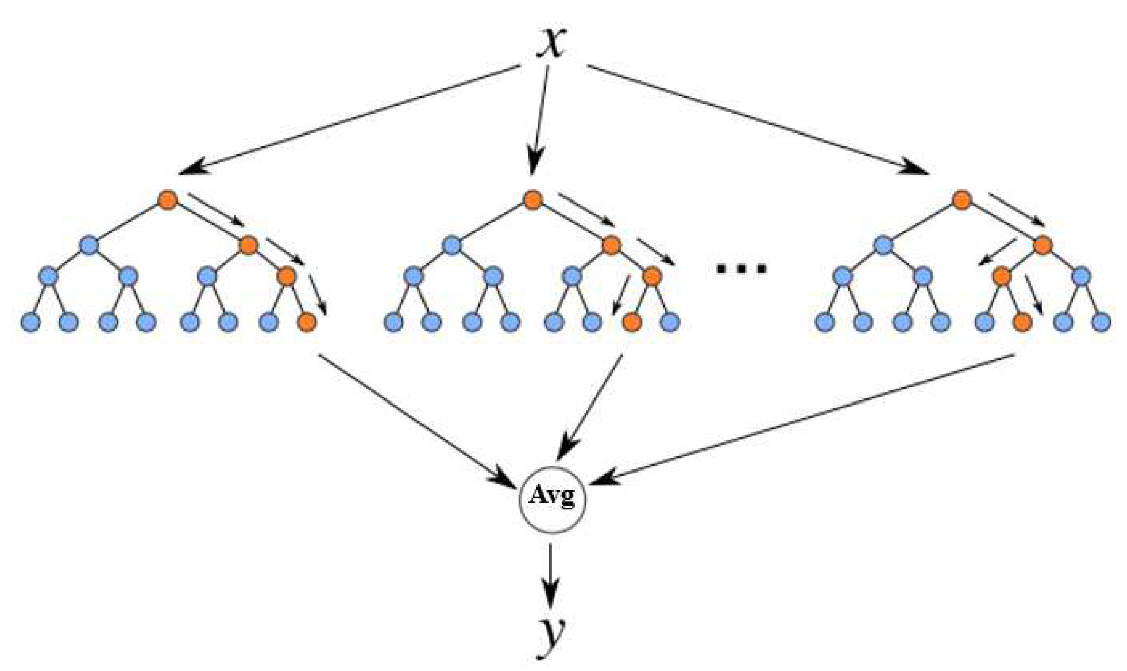
Random Forest is an algorithm that relies on the creation of multiple decision trees during the training process. What distinguishes it from a conventional decision tree is that instead of relying on a single tree structure, Random Forest builds multiple trees using random subsets of data and training features. The purpose is to reduce overfitting and increase the model’s ability to generalize to a variety of situations. In this way, the use of multiple trees gives Random Forest the advantage of dealing with complex and non-linear data, thus improving the accuracy of predictions. In addition, to make final decisions, the algorithm employs a voting method. Each tree in the forest produces an output and these outputs are averaged at the end to obtain the final prediction. The structure of this classifier is represented in
Figure 4.
In the specific context of this paper, 100 trees have been implemented, and each tree has been trained with a random set of data and features, which contributes to the diversity and robustness of the final model.
- 5.
-
YAMNet Deep Neural Network.
In order to study the variation of detection performance with distance with deep learning networks, we have used the deep neural network YAMNet, which is a pre-trained CNN that specializes in the task of audio classification. In this way, using transfer learning techniques, the training and binary classification of our problem is performed.
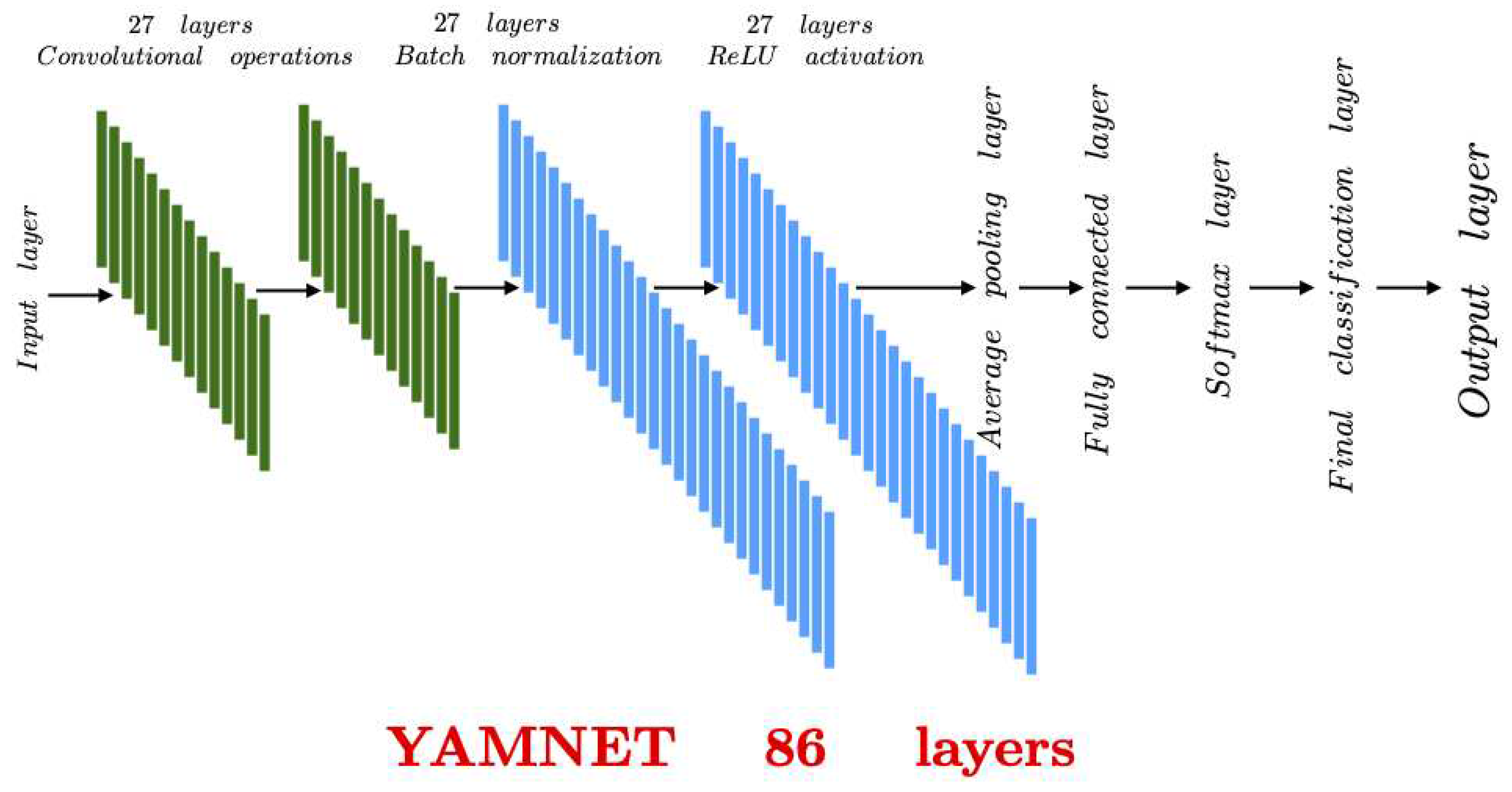
After being trained on the AudioSet-Youtube corpus using the depthwise-separable convolution architecture Movilenet_v1 [
33], YAMNet can predict 521 classes of audio events. This deep neural network is composed of 86 layers, including 27 layers for convolutional operations, 27 layers for batch normalization and ReLU activation, 1 average pooling layer, 1 fully connected layer, 1 softmax layer, and a final classification layer. The final structure of YAMNet is depicted in
Figure 5.
The choice and organization of these layers is not random, but the result of a careful design. The convolutional layers play a key role in extracting meaningful features from the input audio waveforms. Each of these layers is complemented by a batch normalization layer to ensure that the data is properly normalized, avoiding training challenges and improving learning speed. In addition, a ReLU activation function is incorporated after normalization, thus controlling the computational complexity of the network. During the classification phase, a fully connected layer is employed to consolidate information from each neuron between adjacent layers. This approach enables a comprehensive analysis of all input information, facilitating informed and accurate decision making [
34].
Subsequently, if the problem is categorized as a classification issue, similar to the case of the original YAMNet network, a softmax layer is employed that applies a softmax loss function to the input. This allows the actual values to be compared with the predictions and the classification task to be performed. In addition, a final classification layer is used to compute the cross-entropy loss, considering classification tasks and weighted classification with mutually exclusive classes. In contrast, if the problem is considered as a regression problem, the softmax and classification layers are replaced by a final regression layer, which calculates the mean squared error loss by splitting the regression tasks.
4. Materials and Methods
4.1. Database
The database used for design and testing is the same as that used in [
25] and [
26]. This dataset includes audio recordings from several drones, such as the DJI Phantom 3, Cheerson CX 10, Parrot AR, Eachine Racer and Hobbyking FPV250. In addition, it contains sounds that could give rise to false alarms in real situations, because they originate in a similar way, for example due to rotating engines or propellers, such as those generated by airplanes, motorcycles, helicopters, and other less common sounds with similar spectral characteristics to drones, such as those produced by a lawn mower, bulldozers, the Litchfield fire siren and that produced by rolling. It is worth mentioning that the database used in this work has been updated from that used in the previous works, mentioned above; sounds such as the hum of a hairdryer, which, although having similar spectral characteristics, would not be realistic in a genuine environment, have been excluded.
This study focuses on analyzing the degradation of detection as a function of distance. The results obtained when the sensors are close to the source, at a distance of 1 meter, are presented as a reference, to know the limits in detection capability of each detector. Since this is a detection problem, equivalent to a binary classification, the database has been split into two classes: "drones" and "non-drones", with a total of 3512.73 seconds of audio files. Of these, 1919.34 seconds correspond to drone acoustic signals, representing 54.64% of the total, so the database is balanced between the two considered classes.
The audio signals were originally sampled at 24 kHz and 44.1 kHz, but all of them have been resampled to 16 kHz, as there is no relevant information for frequencies above 8 kHz in the signal spectrum.
On the other hand, it is worth mentioning that the detection task (binary classification) would be performed when a sound source has been localized in the environment, using array processing techniques. The use of microphone arrays for the localization task allows the application of spatial filtering techniques for quality enhancement and noise and interference reduction. For this reason, and to make the analysis as realistic as possible, in the database, signals coming from the ground have been attenuated by 20 dB compared to signals captured at another elevation. If the sensor array detects a sound from a drone flying at a certain height, it will not be attenuated by the application of spatial filtering techniques. However, sounds from sources at 0 degree elevations, such as those generated by motorcycles, construction sites, lawn mowers, bulldozers, the Litchfield fire siren, and wheel cuts, are attenuated by 20 dB, as they would have been picked up by a secondary lobe of the microphone array beampattern.
The amplitudes of the signals produced by the UAVs have been scaled, so that the sound pressure level (SPL) is 80 dB for all of them, except for those coming from an elevation angle of 0 degrees, to which an additional 20 dB attenuation is applied, taking into account the application of spatial filtering, as mentioned above. The same procedure has been applied to the background noise signals, adjusting them to a sound pressure level of 40 dB. This choice is based on the assumption that the used sensor array scans the space continuously with a beam narrow enough to achieve good directivity in the measurements. Because of this directivity, it is possible to attenuate noise and interfering signals in other directions, thus confirming that the input noise values are appropriate for the problem in question.
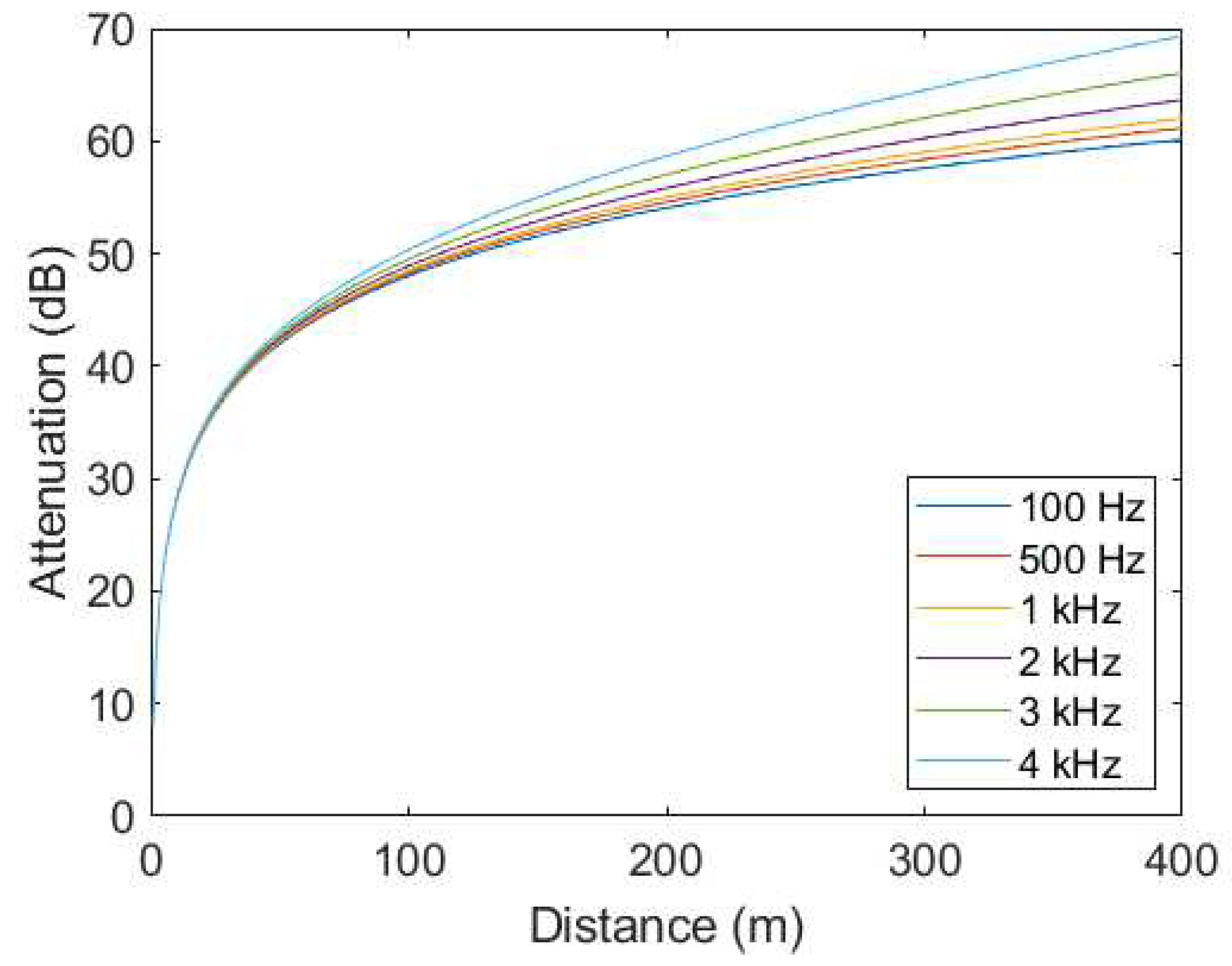
To analyze the performance of the system as a function of distance, a model has been used to estimate the attenuation at a specific distance from the source, as a function of frequency. The model used is defined in the ISO 9613-1 [
27] and 9613-2 [
28] standards, and provides the attenuation suffered by a sound source at a distance, as a function of frequency, and under normal temperature and pressure conditions. In
Figure 6, the attenuation is depicted, as function of distance and frequency, under normal temperature and pressure conditions. During training and testing, this attenuation is only applied to the signal of interest, as the interfering sound sources are considered to be at a fixed distance from the sensor, without any movement.
4.2. Preprocessing for Feature Extraction
The signals have been preprocessed to extract useful features, which will be applied as input vectors to the detectors. Previously, the signal is divided into frames of 512 samples, with an overlap of 50%. Each frame is subjected to an edge enhancement process, and the following spectral characteristics are calculated for each one of them [
29][
31]:
-
Mel Frequency Cepstral Coefficients (MFCC). These coefficients are based on the human peripheral auditory system, so they represent frequency information on a scale that resembles human auditory perception. They are calculated with the following steps [
30]:
- -
Divide the signal in short-time frames.
- -
Apply the Discrete Fourier Transform to each frame and obtain the power spectrum.
- -
Apply a filter bank corresponding to the Mel Scale to the power spectrum obtained in the previous step and add the energies in each of subband.
- -
Take the logarithm of all the energies obtained in the previous step.
- -
Apply the discrete cosine transform to vector of logarithm of power.
The relationship between frequency and the Mel frequency
is expressed in (
6):
Δ-MFCC. These coefficients allow capturing changes in MFCC coefficients as they evolve over time, providing valuable information on how the acoustic properties of sound signals vary at different times. This technique uses least squares to calculate the rate of change of these MFCC features, allowing a more detailed understanding of the temporal variations in the analyzed sound.
Δ-Δ-MFCC. They represent the acceleration of changes in MFCC coefficients as they evolve over time. This involves providing information on the rate of change of the -MFCC coefficients, which adds an additional level of detail on the temporal variations in the acoustic signals. In addition, the ability to analyze the rate of change of the -MFCC coefficients allows them to be combined with other features, improving the accuracy and utility of audio and speech processing applications.
Pitch. It refers to the human perception of the fundamental frequency of a sound, if it exhibits periodicity properties. In the context of our analysis, pitch and fundamental frequency are practically identical, which means that the characteristic we perceive as pitch coincides closely with the fundamental frequency of the sound signal.
Harmonic ratio. It is a measure that represents the ratio between the energy of the harmonics of a sound and the total energy of the signal. It provides information about the harmonic structure of the sound signal.
Spectral roll-off point. A metric that describes the shape of the power spectrum of a signal. It indicates the frequency below which a specific proportion of the total power of the spectrum is found. In other words, this parameter reveals what portion of the signal spectrum is concentrated at frequencies below a given value, thus providing information about the power distribution at different frequencies of the acoustic signal.
Spectral centroid. It is an indicator that describes the center of mass of the frequency spectrum of a signal. That is, it represents the energy-weighted average frequency of the signal, providing information about the spectral distribution of the signal.
Spectral flux. It is a measure that indicates the rate of change of the spectral content of a signal as time elapses, in order to capture abrupt transitions in the spectrum of the acoustic signal.
The mean and standard deviation (std) of the parameters calculated in the different time frames of the signals are obtained. The final set of features are presented in
Table 1, resulting in a total number of 160 features at the end of the process.
4.3. YAMNet Fine-Tuning
In this paper it has been concluded that it is more appropriate to use a YAMNet network with regression rather than classification. This involves predicting continuous values rather than assigning features to predefined classes. This decision is based on the variable and continuous nature of the sounds and noises in our scenario, which requires assessing the similarity of the sound to that of a drone and capturing the continuous variability in the data.
In addition, audio segments with a duration of 0.98 seconds and a sampling rate of 16 kHz have been chosen, following the guidelines of the YAMNet documentation in Matlab. Also, an initial learning rate value of has been selected to ensure stable convergence of the model during training. Through experimentation, it has been determined that 20 epochs are sufficient to effectively address our problem.
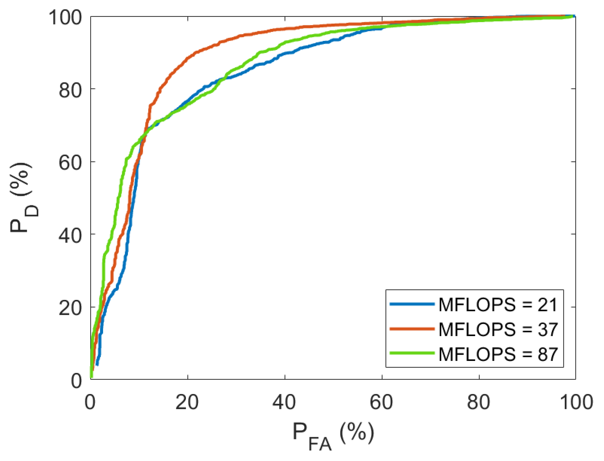
In order to evaluate the number of floating point arithmetic operations that can be performed in one second, the performance measure was varied using Million Floating Point Operations Per Second (MFLOPS) with values of 21, 37 and 87. In addition, we experimented with different numbers of layers in the network to improve efficiency and avoid wasting computational resources. Thus, when a MFLOPS value of 21 is set, only the first 20 layers of the YAMNet network are used. For 37 MFLOPS, the first 40 layers are used, and for 87 MFLOPS, all 83 layers of the network are used. In all scenarios, two final layers are incorporated: a 2D global average pooling layer to reduce the dimensionality of the feature maps before the output layer and a fully connected layer to predict continuous values in regression. In addition, to adapt the problem to our specific binary classification needs, a final layer is included to compute the mean square error of the obtained outputs.
The determination of how many layers to use in our problem was carried out through experimentation.
Figure 7 shows the ROC curve obtained by analyzing the detection problem at a distance of 1 meter between the sound source and the array, i.e. without applying any attenuation. It is observed that the best solution is achieved by using a MFLOPS value of 37, corresponding to 40 layers of the original YAMNet structure. The reason behind not using the full network lies in the fact that YAMNet is pre-trained with a large and diverse data set, which makes the first layers the most likely to learn general features useful for our specific context.
4.4. Performance evaluation using k-fold cross-validation
Finally, to improve the performance evaluation of machine learning and transfer learning models, the k-fold technique (k=10) has been implemented. K-fold cross-validation is a technique for evaluating predictive models [
35]. The dataset is divided into k subsets or folds. The model is trained and evaluated k times, using a different fold as the validation set each time. Performance metrics from each fold are averaged to estimate the model’s generalization performance. This process ensures a more accurate and reliable assessment of performance. By using the complete data set for training and validation, a robust and accurate performance assessment of the different compared systems is obtained.
5. Results and Discussion
This paper evaluates the effectiveness of drone detection with several methods based on machine learning, from simple methods such as linear discriminants, to sophisticated deep networks taking advantage of transfer learning (TL). The experiments performed and the results obtained are presented in this section.
Initially, the learning machines were trained using the database without attenuation, i.e., with data collected at a distance of 1 meter. Nevertheless, the detectors were tested with signals emitted at different distance ranges, to evaluate the capacity of detecting drones at distances different from the distance between the drones and the sensor in the signals used for training. To evaluate the detectors performance, ROC curves were obtained. These curves serve as a graphical representation of the relationship between the true positive rate or probability of detection (), and the false positive rate or probability of false alarm (). Each point of the ROC curve is obtained using a given threshold, the detector outputs are compared with. The higher the for a given , the better the detector for that value. In general, the larger the area under the ROC curve (AUC), the better the detector performance.
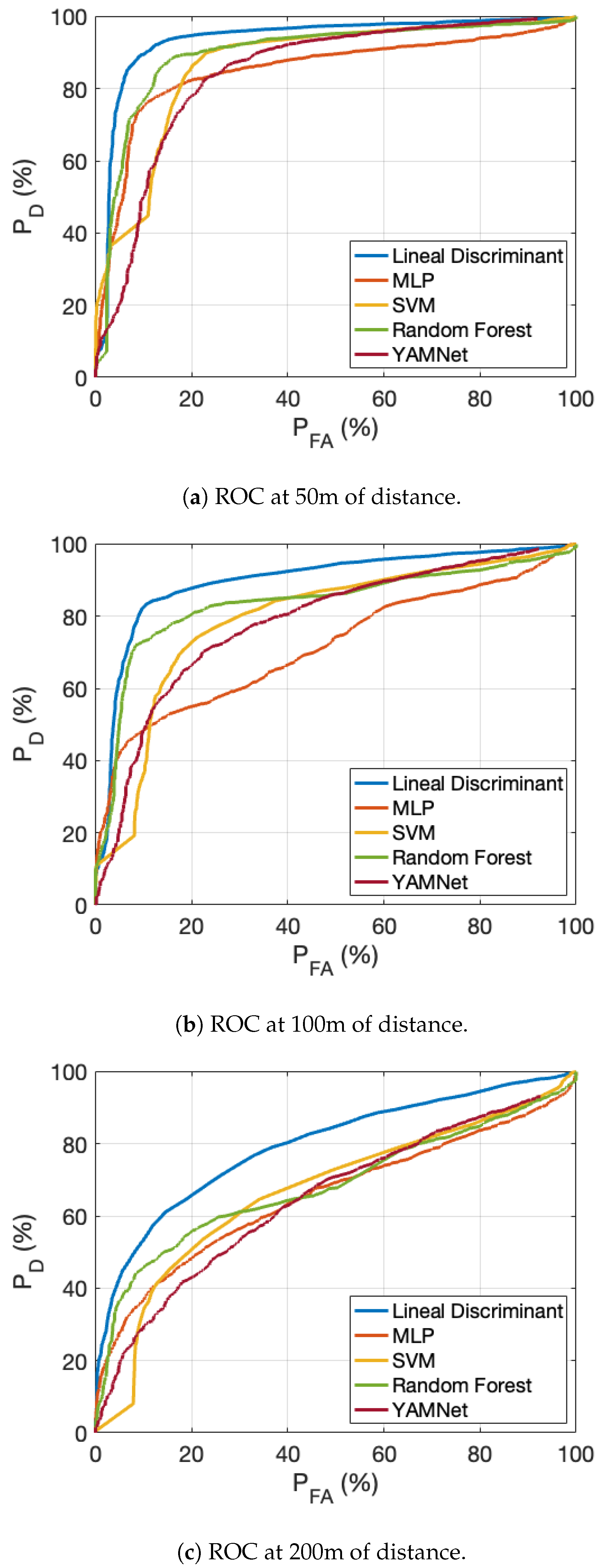
Figure 8a–c are the ROC curves obtained by training the linear discriminant, MLP, SVM, Random Forest and YAMNet with transfer learning, using non-attenuated data. At a distance of 50 meters between the sound source and the microphone array, the AUC is around 90% for the linear discriminant and Random Forest methods, while for the other detectors it is around 80%. These values decrease by approximately 10% when the distance is doubled to 100 meters, for all the detectors but MLP and SVM, whose AUC values are significantly lower. Doubling the distance from the source again (200m), the detection results are still acceptable for the linear classifier, with
values greater than 60% for
values of less than 10%. Therefore, the detector that best generalizes to data obtained at distances different from the distance used to obtain the training data is the simplest detector based on the linear discriminant. Furthermore, with this approach for training, we conclude that acoustic detection is not feasible at distances greater than 200 meters.
After obtaining these results, we trained the model with data attenuated by the effect of distance to simulate real detection conditions. The attenuation is applied in the frequency domain, as it depends on frequency. With this approach, the learning machines are intended to perform well over a larger range of distances, thanks to the fact that data obtained over a wide range of distances between the source and the sensor have been applied during training.
Table 2 shows the percentage of area under the ROC curves, making it easier to compare the methods used.
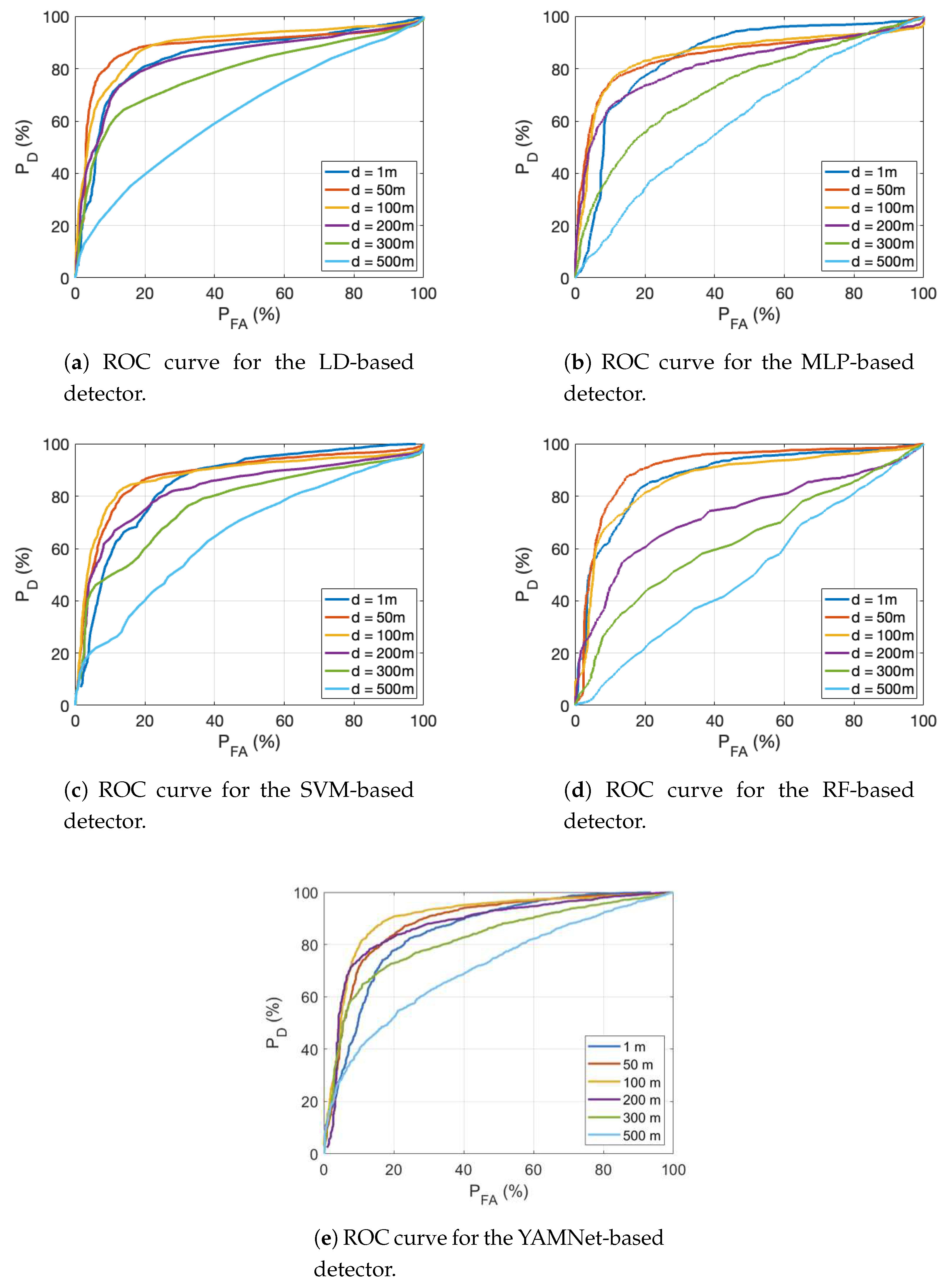
Figure 9a–e present the ROC curves obtained, for all the distance ranges evaluated and for all the detectors considered (note that in this case, each curve plot corresponds to a different detector). At a distance of 100 meters from the source, the AUC is approximately 90% for all detectors. At distances up to 300 meters, the linear discriminant, SVM and YAMNet show similar performance, with an AUC above 80% at 200 meters, decreasing by 5% at 300 meters. However, MLP and Random Forest based detectors are more sensitive to distance, being able to perform acceptable detections only up to 200 meters, but not at longer distances. Finally, as the distance increases up to 500 meters, only the YAMNet-based detector with transfer learning achieves a
of 40 % for a false alarm probability of less than 10%, or in other words, an AUC of about 71%.
The results obtained with a training set that includes audios collected at different distances (therefore, with different attenuation), are in general better than those obtained when training with data collected at a short distance from the source. On the one hand, the detectors perform well at greater distances from the sound source, but on the other hand, the results at short distances are worse. This shows that the detectors perform better overall, but do not reach the detection probabilities that were obtained when training and testing with signals collected in the same distance range.
Therefore, a crucial element in achieving acceptable detection at long distances from the source would be to train with a database that includes sounds and interferences also collected at long distances from the source. With this approach, reliable detections are obtained at distances up to 200 meters for all the detectors studied, up to 300 meters for the simplest detector (linear discriminant), and possibly up to 500 meters for the YAMNet-based detector, which exploits transfer learning.
Another interesting result obtained when training with the data set that includes sounds at all distances considered, is that the performance at the 1 meter distance is worse than the performance at the 50 and 100 meter distances for all the detectors studied. In some cases, such as YAMNet or the detector based on linear discriminants, the detection performance at 200 meters exceeds that obtained without applying attenuation at 1 meter. The conclusion is that the best performance of the detectors trained with this data set occurs when the sound source is at a medium distance from the sensor. Therefore, the approach of including sounds collected at large distances from the sensor in the training data set is suitable for extending the detection range, when only one detector is used.
But the good result obtained when training with sounds recorded at short distances, and testing also with sounds at short distances, suggests that good specialized detectors at a certain distance can be achieved by training exclusively with sounds recorded at that distance. To extend the range of distances, one can think of combining the results with ensembles of detectors, each trained with sounds at a specific range of distances. The application of one or another detector would depend on the result obtained in the localization of the sound source by means of array processing techniques.
These findings are promising and stimulate research into array processing techniques to solve the problem of sound source localization, and to maximize attenuation of interferers. These advances are essential to achieve a final solution that allows detection at wide ranges of distances with high AUC. In addition, the possibility of developing specialized detectors for each distance range, which would be selected based on the information provided by a localization system based on microphone arrays, has been proposed and will be explored in future works. Taken together, these results suggest that acoustic detection can be considered as a competitive and complementary method to detections obtained with other types of sensors.
6. Conclusion
In this study, the acoustic detection performance of drones at different distances has been comprehensively evaluated, providing valuable insights for future research and practical applications. The evaluation has been performed by extracting relevant features in the frequency domain and applying machine learning methods, together with the transfer learning technique using the YAMNet network. For the application of these methods a carefully designed database including drone sounds and interferences has been used, simulating realistic conditions by specific attenuation of the interferences.
The results show that the distance variation has a significant impact on the detection results, due to the attenuation that occurs in the sound propagation, which is also frequency dependent. In addition, the detectors performance depends on the training data set used. When a training set is used in which the data is not attenuated, good detection results are achieved at distances up to 200 meters. In contrast, if the training set includes sounds at different distances, detection results improve significantly at medium and long distances, allowing detection at distances up to 500 meters with the best type of detector. These results underline the importance of taking into account the diversity of distances when forming training sets, highlighting that this aspect is crucial to achieve accurate and efficient detection.
As future research perspectives, it is essential to investigate advanced array processing techniques to improve interference reduction through spatial filtering and to achieve precise localization of sound sources, which can serve as input to a system that allows selecting the best detector. for the distance at which the source is located.
In addition, it is necessary to develop machine learning and transfer learning models capable of handling distance variations with high precision. It is considered crucial to expand the constructed database to avoid possible biases and improve generalization to new data. More thorough preprocessing of the input data is also emerging as a fundamental improvement to minimize noise as much as possible.
However, the fact that the best results are obtained with a deep network like YAMNet suggests research with networks of this type. To train these networks, it is necessary to have enormous amounts of data, which cannot be easily achieved in real environments. For this reason, research into techniques for increasing the number of data is also considered.
This study not only expands our understanding of drone acoustic detection, but also suggests that this technology has the potential to be a valuable tool in real-world applications. By complementing other detection methods, it can provide comprehensive and reliable solutions in various environments, marking a significant advancement in the field of acoustic drone detection.
Author Contributions
Conceptualization, Diana Tejera-Berengué, Manuel Utrilla-Manso and Manuel Rosa-Zurera; Data curation, Diana Tejera-Berengué, FangFang Zhu-Zhou and Roberto Gil-Pita; Formal analysis, Diana Tejera-Berengué, FangFang Zhu-Zhou and Manuel Utrilla-Manso; Funding acquisition, Roberto Gil-Pita and Manuel Rosa-Zurera; Investigation, Diana Tejera-Berengué, FangFang Zhu-Zhou and Roberto Gil-Pita; Methodology, Diana Tejera-Berengué, FangFang Zhu-Zhou and Roberto Gil-Pita; Project administration, Roberto Gil-Pita and Manuel Rosa-Zurera; Resources, Diana Tejera-Berengué, Roberto Gil-Pita and Manuel Rosa-Zurera; Software, Diana Tejera-Berengué and Roberto Gil-Pita; Supervision, Manuel Utrilla-Manso, Roberto Gil-Pita and Manuel Rosa-Zurera; Validation, Diana Tejera-Berengué, Roberto Gil-Pita and Manuel Rosa-Zurera; Visualization, Diana Tejera-Berengué, Manuel Utrilla-Manso and Manuel Rosa-Zurera; Writing – original draft, Diana Tejera-Berengué and Manuel Rosa-Zurera; Writing – review & editing, Diana Tejera-Berengué and Manuel Rosa-Zurera.
Funding
This work is part of the project PID2021-129043OB-I00 funded by MCIN/AEI/10.13039/ 501100011033/FEDER, UE, and projects SBPLY/19/180501/000350 funded by the Regional Government of Castilla La Mancha, and EPU-INV/2020/003, funded by the Community of Madrid and University of Alcala. This paper is an expanded paper from the IEEE Sensors Applications Symposium held on July 18-20, 2023 in Ottawa, Canada.
Conflicts of Interest
The authors declare no conflict of interest.
Abbreviations
The following abbreviations are used in this manuscript:
| UAV |
Unmanned aerial vehicle |
| SVM |
Support vector machine |
| MFCC |
Mel-frequency cepstral coefficients |
| RNN |
Recurrent neural network |
| CNN |
Convolutional neural network |
| CRNN |
Convolutional recurrent neural network |
| HERM |
Helicopter rotor modulation |
|
Probability of detection |
|
Probability of false alarm |
| ROC |
Receiver operating characteristic |
| LD |
Linear discriminant |
| RMSE |
Root mean square error |
| MLP |
Multilayer perceptron |
| RBF |
Radial basis function |
| RF |
Random Forest |
| ReLU |
Rectified linear unit |
| SPL |
Sound pressure level |
| ISO |
International Organization for Standardization |
| std |
Standard deviation |
| MFLOPS |
Million floating point operations per second |
| AUC |
Area under the curve |
| TL |
Transfer learning |
References
- V. Chamola, P. Kotesh, A. Agarwal, N. Gupta, M. Guizani, et al. A comprehensive review of unmanned aerial vehicle attacks and neutralization techniques. Ad hoc networks, 111:102324, 2021. Elsevier.
- I. Guvenc, F. Koohifar, S. Singh, M. L. Sichitiu, D. Matolak. Detection, tracking, and interdiction for amateur drones. IEEE Communications Magazine, 56(4):75-81, 2018. IEEE.
- M. A. Khan, H. Menouar, A. Eldeeb, A. Abu-Dayya, F. D. Salim. On the detection of unauthorized drones—Techniques and future perspectives: A review. IEEE Sensors Journal, 22(12):11439-11455, 2022. IEEE.
- Q. Cheng, X. Li, B. Zhu, Y. Shi, B. Xie. Drone Detection Method Based on MobileViT and CA-PANet. Electronics 2023, 12(1):223, 2023. MDPI.
-
Dual-Source Detection and Identification System Based on UAV Radio Frequency Signal. IEEE Transactions on Instrumentation and Measurement, 70(2006215):1-15, 2021. IEEE.
- E. E. Case, A. M. Zelnio, B. D. Rigling. Low-cost acoustic array for small UAV detection and tracking. 2008 IEEE National Aerospace and Electronics Conference, pages 110-113, 2008. IEEE.
- J. Kim, C. Park, J. Ahn, Y. Ko, J. Park, J. C. Gallagher. Real-time UAV sound detection and analysis system. 2017 IEEE Sensors Applications Symposium (SAS), pages 1-5, 2017. IEEE.
- Yang, E. T. Matson, A. H. Smith, J. E. Dietz, J. C. Gallagher. UAV Detection System with Multiple Acoustic Nodes Using Machine Learning Models. 2019 Third IEEE Int. Conf. on Robotic Computing (IRC), pages 493-498, 2019. IEEE.
- J. Mezei, V. Fiaska, A. Molnár. Drone sound detection. 16th IEEE Int. Symposium on Computational Intelligence and Informatics (CINTI), pages 333-338, 2015. IEEE.
- B. Yang, E. T. Matson, A. H. Smith, J. E. Dietz, J. C. Gallagher. UAV detection system with multiple acoustic nodes using machine learning models. 2019 Third IEEE International Conference on Robotic Computing (IRC), pages 493-498, 2019. IEEE.
- A. Bernardini, F. Mangiatordi, E. Pallotti, L. Capodiferro. Drone detection by acoustic signature identification. Electronic Imaging, 2017(10):60-64, 2017. Society for Imaging Science and Technology. 2017.
- S. Al-Emadi, Abdulla Al-Ali, A. Mohammad, Abdulziz Al-Ali. Audio based drone detection and identification using deep learning. 15th Int. Wireless Communications and Mobile Computing Conference (IWCMC), pages 459-464, 2019. IEEE.
- Y. Seo, B. Jang, S. Im. Drone detection using convolutional neural networks with acoustic STFT features. 2018 15th IEEE International Conference on Advanced Video and Signal Based Surveillance (AVSS), pages 1-6, 2018. IEEE.
- Q. Dong, Y. Liu, X. Liu. Drone sound detection system based on feature result-level fusion using deep learning. Multimedia Tools and Applications, 82(1):149-171, 2023. Springer Nature.
- D. Utebayeva, L. Ilipbayeva, E.T. Matson. Practical Study of Recurrent Neural Networks for Efficient Real-Time Drone Sound Detection: A Review. Drones, 7(1):26, 2022. MDPI.
- H. Dong, J. Liu, C. Wang, H. Cao, C. Shen, J. Tang. Drone Detection Method Based on the Time-Frequency Complementary Enhancement Model. IEEE Transactions on Instrumentation and Measurement (in press), 2023. IEEE.
- M. Yaacoub, H. Younes, M. Rizk. Acoustic Drone Detection Based on Transfer Learning and Frequency Domain Features. 2022 International Conference on Smart Systems and Power Management (IC2SPM), pages 47-51, 2022. IEEE.
- P. Casabianca, Y. Zhang. Acoustic-based UAV detection using late fusion of deep neural networks. Drones, 5(3):54, 2021. MDPI.
- B. Taha, A. Shoufan. Machine learning-based drone detection and classification: State-of-the-art in research. IEEE access, 7:138669-138682, 2019. IEEE.
- U. Seidaliyeva, L. Ilipbayeva, K. Taissariyeva, N. Smailov, E.T. Matson. Advances and Challenges in Drone Detection and Classification Techniques: A State-of-the-Art Review. Sensors, 2024: 24, 125, 2023. MDPI. Sensors.
- J. Neyman, E. S. Pearson. On the problem of the most efficient tests of statistical hypotheses. Philosophical Transactions of the Royal Society of London. Series A, 231(694-706):289-337, 1933.
- M. P. Jarabo-Amores, M. Rosa-Zurera, R. Gil-Pita, F. Lopez-Ferreras. Study of two error functions to approximate the Neyman–Pearson detector using supervised learning machines. IEEE Transactions on Signal Processing, 57(11):4175-4181, 2009. IEEE.
- M. P. Jarabo-Amores, D. de la Mata-Moya, R. Gil-Pita, M. Rosa-Zurera. Radar detection with the Neyman–Pearson criterion using supervised-learning-machines trained with the cross-entropy error. EURASIP Journal on Advances in Signal Processing, 2013:1-10, 2013. EURASIP.
- D. de la Mata-Moya, M. P. Jarabo-Amores, J. M. de Nicolás-Presa, M. Rosa-Zurera. Approximating the Neyman–Pearson detector with 2C-SVMs. Signal Processing, 131:364-375, 2013. Elsevier.
- J. García-Gómez, M. Bautista-Durán, R. Gil-Pita, M. Rosa-Zurera. Feature selection for real-time acoustic drone detection using genetic algorithms. Audio Engineering Society Convention 142, 2017. Audio Engineering Society.
- D. Tejera-Berengue, F. Zhu-Zhou, M. Utrilla-Manso, R. Gil-Pita, M. Rosa-Zurera. Acoustic-Based Detection of UAVs Using Machine Learning: Analysis of Distance and Environmental Effects. 2023 IEEE Sensors Applications Symposium (SAS), pages 1-6, 2023. IEEE.
- International Organization for Standardization. Acoustics: Attenuation of Sound During Propagation Outdoors. 1993. International Organization for Standardization.
- International Organization for Standardization. Acoustics-Attenuation of Sound During Propagation Outdoors: Part 2: General Method of Calculation. 1996. International Organization for Standardization.
- G. Tzanetakis, P. Cook. Marsyas: A framework for audio analysis. Organised sound, 4(3):169-175, 2000.
- S. Davis, P. Mermelstein. Comparison of parametric representations for monosyllabic word recognition in continuously spoken sentences. IEEE transactions on acoustics, speech, and signal processing, 28(4): 357-366, 1980.
- R. Serizel, V. Bisot, S. Essid, G. Richard. Acoustic Features for Environmental Sound Analysis. Computational Analysis of Sound Scenes and Events. Springer, Cham, 2018.
- O. L. Mangasarian, D. R. Musicant. Lagrangian support vector machines. Journal of Machine Learning Research, 1(Mar):161-177, 2001.
- A. G. Howard, M. Zhu, B. Chen, D. Kalenichenko, W. Wang, T. Weyand, M. Andreetto, H. Adam. Mobilenets: Efficient convolutional neural networks for mobile vision applications. arXiv preprint arXiv:1704.04861, 2017. arXiv:1704.04861, 2017.
- K. K. Mohammed, E. I. Abd El-Latif, N. Emad El-Sayad, A. Darwish, A. Ella Hassanien. Radio frequency fingerprint-based drone identification and classification using Mel spectrograms and pre-trained YAMNet neural. Internet of Things, 23:100879, 2023. Elsevier.
- T. Fushiki. Estimation of prediction error by using K-fold cross-validation. Statistics and Computing, 21:137-146, 2011.
|
Disclaimer/Publisher’s Note: The statements, opinions and data contained in all publications are solely those of the individual author(s) and contributor(s) and not of MDPI and/or the editor(s). MDPI and/or the editor(s) disclaim responsibility for any injury to people or property resulting from any ideas, methods, instructions or products referred to in the content. |
© 2024 by the authors. Licensee MDPI, Basel, Switzerland. This article is an open access article distributed under the terms and conditions of the Creative Commons Attribution (CC BY) license (http://creativecommons.org/licenses/by/4.0/).
 In this paper, we have chosen to use a perceptron with a single hidden layer, since it can approximate any discriminant function if a sufficient number of neurons in that hidden layer are used. The neurons in this layer are connected to the output, and this output is compared with a predefined threshold to make decisions in the detection and classification process. We have used the Quasi-Newton-based backpropagation training algorithm, where the connection weights are adjusted at each iteration or epoch in batch mode, i.e., using subsets of training data instead of the full set. This not only reduces the computational burden, but also significantly speeds up the training process.