Preprint

Article

Rapid Determination Method of Reinforced Concrete Column Failure Modes using Simple Structural Information

Altmetrics

Downloads

130

Views

Comments

A peer-reviewed article of this preprint also exists.

Subin Kim,

Hee-Jin Hwang,Keunyeong Oh,

Jiuk Shin^*

Subin Kim,

Hee-Jin Hwang,Keunyeong Oh,

Jiuk Shin^*

This version is not peer-reviewed

Submitted:

07 January 2024

Posted:

08 January 2024

You are already at the latest version

Alerts

Abstract

Existing reinforced concrete buildings with seismically-deficient column details affect the overall behavior depending on the failure type of column. The purpose of this study is to develop and validate a machine learning-based prediction model for the column failure modes (shear, flexure-shear and flexure failure modes). For this purpose, artificial neural network (ANN), K-nearest neighbor (KNN), decision tree (DT), and random forest (RF) models were used considering previously-collected experimental data. Using four machine learning methodologies, we developed a classification learning model that can predict the column failure modes in terms of the input variables using concrete compressive strength, steel yield strength, axial load ratio, height-to-dept aspect ratio, longitudinal reinforcement ratio, and transverse reinforcement ratio. The performance of each machine learning model was compared and verified by calculating accuracy, precision, recall, F1-Score, and ROC. Based on the performance measurements of the classification model, the RF model represents the highest average value of the classification model performance measurements among the considered learning methods, and it can conservatively predict the shear failure mode. Thus, the RF model can rapidly predict the column failure modes with the simple column details. Additionally, it was demonstrated that the predicted failure modes from the selected model were exactly same as the failure mode determined from a code-defined equation (traditional method)

Keywords:

Subject: Engineering - Civil Engineering

1. Introduction

Determining the failure mode of reinforced concrete (RC) columns is a crucial component in the performance evaluation process of buildings and bridges, and it is closely related to structural safety and rapid strength reduction. In RC frame structures built before the implementation of seismic design, the failure mode of the columns can impact the overall structure behavior. Structural engineers must consider reinforcement methods for columns with existing seismic vulnerabilities, particularly those with inadequate structural details. The failure mode of columns is influenced by various structural details (longitudinal reinforcement ratio, transverse reinforcement ratio, etc.) and geometric characteristics (column length, boundary conditions, etc.). This has been verified through various previously conducted experimental studies [1,2,3].

Zhu et al. [4] attempted to classify the failure modes of RC columns using the shear strength of stirrups. Qi et al. [5] considered parameters such as the shear span to depth ratio, and hoop spacing to depth ratio. Various variables reflecting the failure modes of columns have been investigated via experimental studies. Based on the findings of these studies, standards have been developed, proposing an experiment-based equation to calculate the shear capacity of columns. To determine the failure mode of these columns, comparisons between nonlinear static pushover analysis based on fiber elements and the code-based shear capacity equation specified by American Society of Civil Engineering (ASCE) 41-23 may be necessary. To quickly assess the failure modes of columns, this study utilized a machine learning approach considering several parameters for the column details.

Machine learning models for predicting the failure modes of RC structures have been previously investigated. For example, the performance of artificial neural networks (ANNs) was evaluated in several previous studies considering their application toward the strength prediction of RC columns [6] or seismic research on RC frames [7]. Alibrandi et al. [8] evaluated the failure probability of structures using a support vector machine (SVM) approach among classification techniques. This technique was subsequently used by Mangalathu & Jeon [9] to classify the failure modes in RC beam-column joints. Another machine learning model that can be utilized in practice without complex calculations is the decision tree (DT). In a previous study, the DT model classified the failure modes in RC joints [10]. Because the failure modes of columns vary depending on the overall strength [11], energy dissipation capacity, and ductility of RC columns [12], failure grades can be used to aid engineers in selecting optimized characteristics to prevent hazardous failures. Mangalathu et al. [13] proposed a RF model for predicting failure modes of RC columns and shear walls, and conducted a study to identify and rank important variables affecting failure modes. The RF models provide more than 80 % accuracy for testing dataset for columns and shear walls. Additionally, Feng & Jiang [14] investigated the use of ensemble machine learning or more specifically, adaptive boosting (AdaBoost) algorithm, to predict the failure modes and bearing capacity in rectangular RC columns with 18 detailed input parameter. As compared to the previous study, this study developed the machine-learning based model with the simpler structural details predicting the column failure modes.

This study proposes a machine-learning-based model to rapidly predict the failure modes of RC columns using simple input parameters. This study utilizes a database of 330 experimental tests on RC columns, incorporating six key input variables (i.e., concrete compressive strength, steel yield strength, axial load ratio, height-to-depth aspect ratio, longitudinal reinforcement ratio, and transverse reinforcement ratio) that can influence the failure behavior of RC columns. The results obtained using the machine-learning-based model are compared with those from structural analysis and equations provided in various standards to verify the performance of the proposed system. This study aims to analyze the performances of various machine learning techniques for predicting the difference failure modes (flexure, flexure-shear, and shear failure) of RC columns and to determine the best prediction model.

2. Experimental Database

This section describes the database used for machine learning and the key variables influencing the failure behavior of RC columns.

2.1. Reinforced Concrete Column Database

In this study, a prediction model was developed for rectangular RC columns using a total of 330 data points. A collection of experimental results on 330 rectangular RC columns published in reports by the American Concrete Institute (ACI) and the Pacific Earthquake Engineering Research Center (PEER) [15] was used. The database comprises flexure, flexure-shear, and shear failure modes. Previous research has shown these three modes of failure in RC columns occur due to degradation in the lateral load performance following cracking [16]. Definitions of flexure, flexure-shear, and shear failure are presented in Table 1 [17]. Due to the costly and time-consuming nature of experimental methods for evaluating RC column failure modes, alternative practical techniques are required. 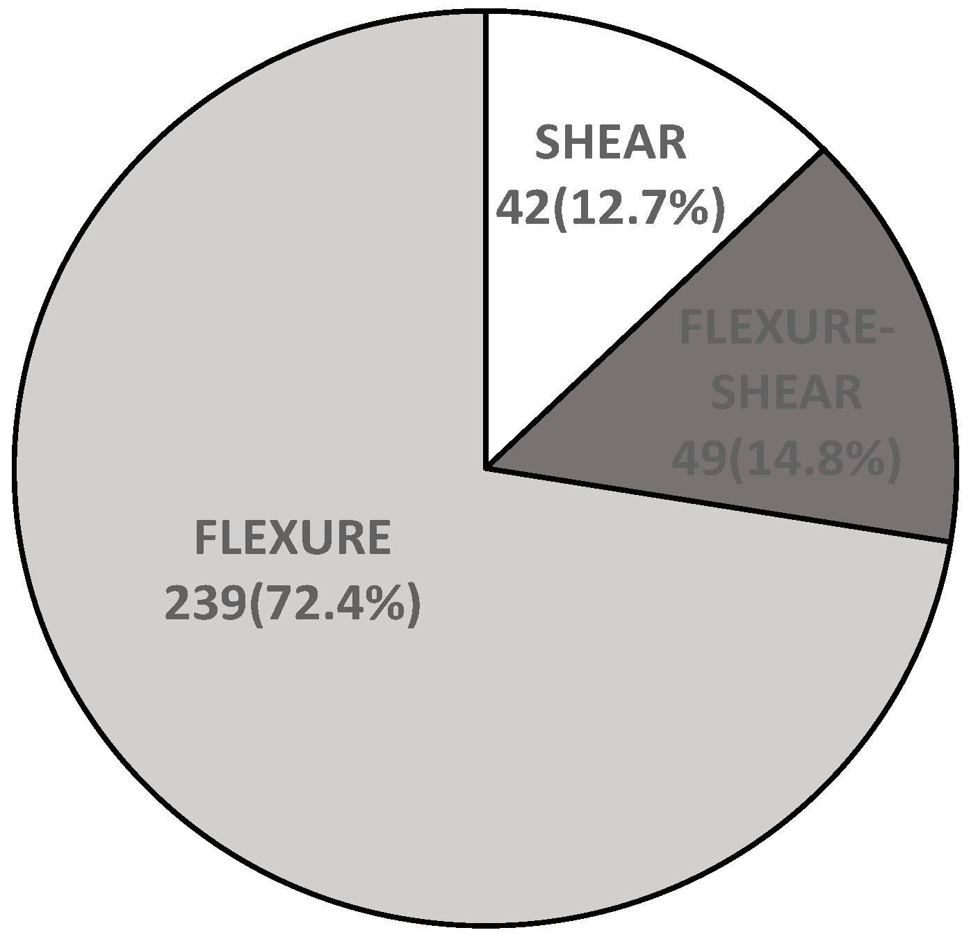Figure 1 illustrates the components of the RC column database used in this study.

2.2. Input Variables Influencing Failure Behavior

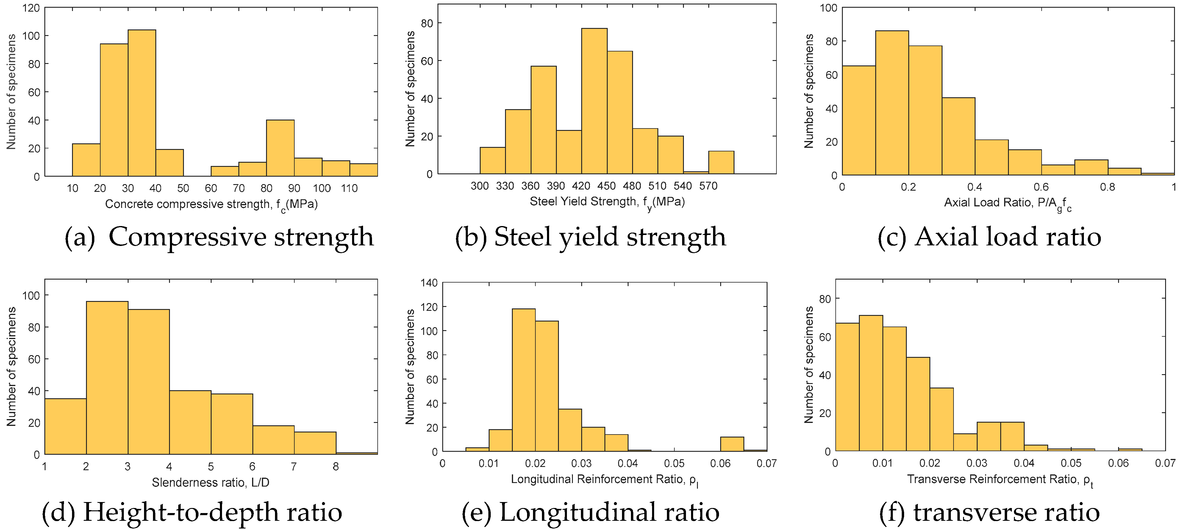
In this study, the input variables are the concrete compressive strength (f_c), steel yield strength (f_y), axial load ratio (P/A_gf_c), height-to-depth aspect ratio (L/D), longitudinal reinforcing ratio (ρ_l), and transverse reinforcing ratio (ρ_t). Figure 2 shows the distribution of the six input variables used in the RC column database.

Concrete and steel strengths were selected as input variables to predict failure modes with different strength values. Previously, Choi et al. [18] demonstrated that the shear strengths of RC columns increases with increasing concrete strength and axial stress. The shear strength is known to increase with increasing axial load, as indicated by the following equation:

V_{A C I} = \frac{1}{6} (1 + \frac{N_{u}}{14 A_{g}}) \sqrt{f_{c}} b_{w} d + \frac{A_{v} f_{y} d}{s}

(1)

where N_u is the axial load (N) acting perpendicular to the cross-section simultaneously with V_u, A_g is total cross-sectional area of the column (mm²), fc is the designed compressive strength of the concrete (MPa), b_w is the web width of the member (mm), d is the effective depth of the column (mm), A_v is the total cross-sectional area of the transverse reinforcement within spacing (mm²), f_y is the designed yield strength of the reinforcement (MPa), and s the spacing of the transverse reinforcement (mm). Bažant & Kwon [19] demonstrated that as the slenderness ratio of a column increases, the size effects become more pronounced and the brittleness increases. Shi et al. [20] demonstrated that an increase in the longitudinal reinforcing ratio enhances flexural strength, but has little impact on displacement, while an increase in the transverse reinforcing ratio strengthens the column and improves its energy dissipation capacity. Table 2 shows the minimum, maximum, and nominal values of the input variables. The nominal values were determined based on statistical data, representing the average values within the most concentrated range of data points. Because there are no cases with an axial load ratio of 0, the minimum value was selected to be the smallest value after 0.

3. Machine Learning Methodology

Machine learning is a process in which computers analyze and learn from data that is inputted into a mathematical model, recognizing patterns to predict target values. Supervised learning uses a secured dataset to train a model, which then predicts new data. If the data is continuous, regression techniques are used; if the data is discrete, classification techniques are applied. In this study, classification techniques are employed to predict failure behavior. The data is divided into two sets: training and test datasets. The training dataset is used to uncover potential predictive relationships, while the test dataset is used to assess the efficiency and accuracy of the predictive model. The advantage of this technique is that the machine learning model can be tested on data that is not included in the training model, and it is possible to evaluate whether the model has overfitted the data. This study employs ANN, K-nearest neighbor (KNN), decision tree (DT), and random forest (RF) machine learning techniques.

ANN is one of the most widely used models in this field. ANNs use a set of independent variables (input variables) to estimate the values of dependent variables (target variables). These systems aim to simulate how human brains and neurons interact in a simplified manner. A neural network typically consists of three layers: the input, hidden, and output layers. Each layer has nodes (neurons) that determine the output based on weighted inputs and biases considering the transfer function. These neurons determine the output parameters of the ANN. Due to the complexity of the matrix calculations in neural networks, it is impossible to obtain a simple solution (e.g., a linear equation) based on the final structure of an ANN. To achieve an optimal training model, hyperparameters are used, which include the size of the hidden layers, activation functions of the hidden layers, batch size, and maximum number of iterations.

KNN is a non-parametric method for classifying data into groups. A KNN classification model assigns a weight of 1/k to the K-nearest neighbor and a weight of 0 to all other neighbors. For a positive integer k and a test observation datapoint x, the classifier identifies the k points that are closest to x in the dataset. The choice of k has a significant impact on the learning performance of this system; a high k value can lead to underfitting errors due to difficulty in clearly expressing data features, while a low k value can lead to overfitting errors influenced by specific data. The hyperparameters in KNN systems include the number of neighbors, method of measuring neighbor distance, distance weighting function, and method used to search for the nearest neighbor.

The use of DT is a non-parametric approach for classifying data, offering an efficient, accurate, and uncomplicated computational approach. The algorithm creates a tree-shaped graph based on the training data. In a decision tree, responses can be predicted according to the decisions made from the start node to the end node. Each node is associated with a test condition, and each branch represents the result of a test. In decision trees, a series of data is first provided to the machine learning algorithm to find the most suitable tree for the classification objective. This structure employs a comparative approach that sets boundaries for each independent variable (classifier) based on observed outcomes. By comparing each step and following the branches, it is possible to determine the label of the input vector (i.e., the error class in this study). The hyperparameters in decision trees include the maximum tree depth, maximum number of decision splits, and minimum number of observations for leaf/branch nodes.

Ensemble learning is a method that utilizes multiple learning models to train data, as opposed to training with a single machine-learning model. Common approaches include voting, bagging, boosting, and stacking. RF is an ensemble model for decision trees, combining several trees with different characteristics to produce results as a collective model. The hyperparameters in RF include the number of decision trees, minimum amount of sample data required for node splitting, and maximum depth of the trees.

In this study, the four machine learning models were utilized. For the input variables, concrete compressive strength was randomly distributed between 13.10 MPa and 118.00 MPa. The yield strength of reinforcement was distributed between 0 MPa and 587.10 MPa, axial force ratio varied between 0.03 and 0.9, confining ratio ranged from 1.12 to 8.67, main reinforcement ratio was distributed between 0.0009 and 0.0615, and shear reinforcement ratio was randomly distributed between 0.0068 and 0.0694. Machine learning was conducted using these input variables, and the optimization process was carried out for each machine learning model. To develop and validate the machine-learning models, more than 80 % of experimental dataset (255 data points) was utilized for training, and the rest of them was tested for validating the developed models. The hyperparameters of the ANN were adjusted for hidden layer size and activation functions, and the KNN’s hyperparameters were adjusted for the number of neighbors and the method for measuring distances. The DT hyperparameters were adjusted for the minimum number of observations in a leaf node and the maximum tree depth. The RF hyperparameters were adjusted for maximum tree depth, the number of iterations in training, and the learning rate. Table 3 summarized hyperparameters for ANN, KNN, DT, and RF optimized with minimum variation between actual and predicted values varying each hyperparameters in 30 iteration steps.

4. ML-based Classification Model for the Determination of Column Failure Modes

In this study, the most suitable model was selected using classification model performance indicators to evaluate the performance of the RC column failure-mode prediction models. The performance indicators used to evaluate the classification models include the accuracy, precision, recall, F1-score, and area under the curve (AUC), which can be determined using a confusion matrix.

Table 4 illustrates the basic concept of a confusion matrix. When classifying flexure failure (positive) and shear failure (negative), a true negative (TN) value is identified when the actual shear failure is correctly predicted as shear failure, and a true positive (TP) value is determined when the actual flexure failure is predicted as flexure failure. A false negative (FN) occurs when the actual flexure failure is incorrectly predicted as shear failure, and a false positive (FP) occurs when the actual shear failure is incorrectly predicted as flexure failure. These prediction outcomes are used to determine the accuracy (ratio of correctly predicted cases to the total predictions), precision (ratio of actual flexure failures among those predicted as flexure failures), recall (ratio of actual flexure failures predicted as such), and F1-score (harmonic mean of recall and precision), which are calculated using Equations (2) to (5), respectively. Increasing precision tends to decrease recall and vice versa, creating a trade-off relationship. The receiver operating characteristic (ROC) curve is a graph plotted with sensitivity and 1-specificity. Here, sensitivity is the same as recall, and specificity is calculated using Equation (6). AUC refers to the area under the ROC curve. A superior classification model is characterized by an AUC value close to 1, and its graph tends to approach the top left corner.

A c c u r a c y = \frac{(T P + T N)}{(T P + T N + F P + F N)}

(2)

P r e c i s i o n = \frac{T P}{(T P + F P)}

(3)

R e c a l l = \frac{T P}{(T P + F N)}

(4)

F 1 - s c o r e = \frac{2 \times P r e c i s i o n \times R e c a l l}{(P r e c i s i o n + R e c a l l)}

(5)

S p e c i f i c i t y = \frac{T N}{(T N + F P)}

(6)

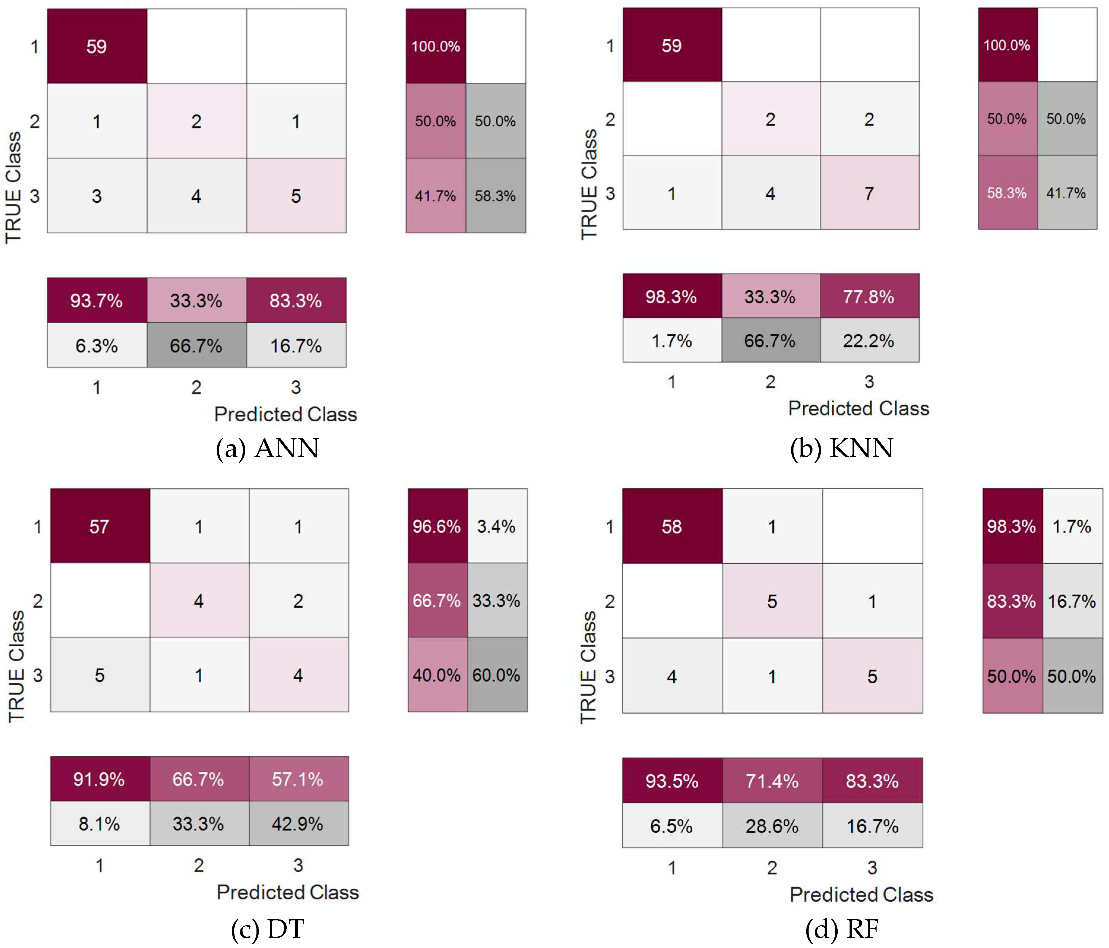
Figure 3 shows the confusion matrices for each machine learning model used in this study. A confusion matrix allows compare actual classes for given input variables with the predicted classes from the machine learning model for the same input variables. In the confusion matrix of this study, the label 1 to 3 means flexural failure, shear failure, and flexural-shear failure types, respectively. The columns of the matrix represent predicted classes, ant the rows indicate actual classes. Cells along the diagonal indicate correctly classified observations. For example, in the case of the ANN model, it can be observed that out of 59 data points known to be of the flexural failure type, 59 were correctly classified as flexural failure type. Out of 4 data points known to be of the shear failure type, 2 were correctly classified as shear failure type, one was misclassified as flexural failure type, and one as flexural-shear failure type. Among the 12 data points known to be of the flexural-shear failure type, 5 were correctly classified as flexural-shear failure type, 3 were misclassified as flexural failure type, and 4 as shear failure type. For the ANN and KNN models, the overall precision, recall, and F1-scores for shear failure modes are below average, whereas these metrics for flexure failure modes are above average. Therefore, flexure failure modes can be accurately predicted, but predictions for shear failure modes are not accurate. The DT model generally shows below average precision, recall, and F1-scores for shear failure and flexure-shear failure modes, while these metrics for flexure failure modes are above average. Therefore, the DT model can accurately predict flexure failure modes, but not shear and flexure-shear failure modes. The RF model demonstrates above-average precision, recall, and F1-scores for flexure failure modes, while precision and F1-scores for shear failure modes, excluding recall, are below average. Additionally, for flexure-shear failure modes, recall and F1-scores, excluding precision, are below the average values. Therefore, flexure failure modes are accurately predicted, but predictions for shear failure modes can be considered conservative.

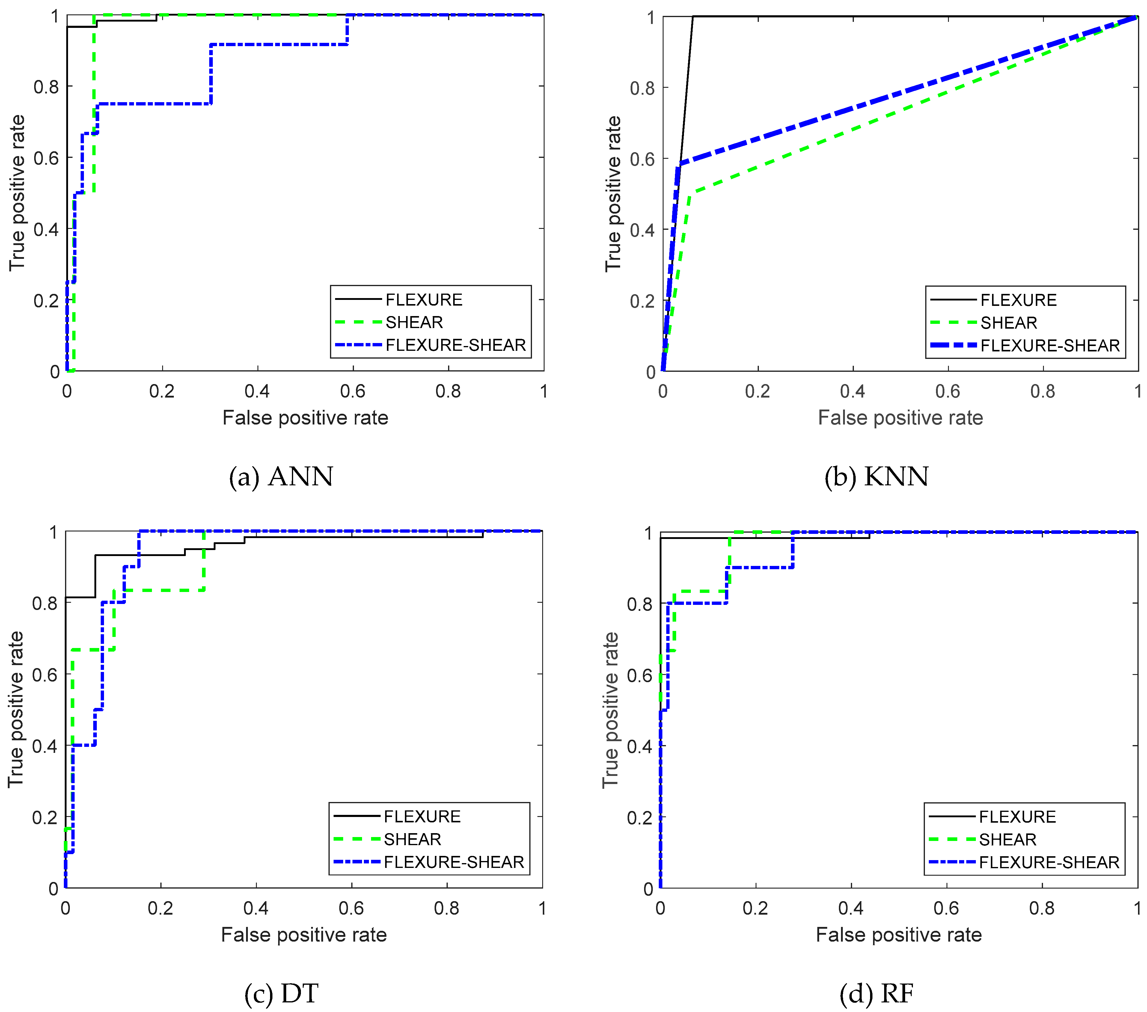
Figure 4 displays the ROC curves for each machine learning model investigated in this study. Excluding the KNN model, the other three models show high AUC values. The AUC values for the flexural failure type are more than 0.95 for all four models. Similarly, the AUC values for shear failure type and flexural-shear failure type are more than 0.85 for all models except KNN.

Table 5 presents the accuracy, precision, recall, F1-score, and AUC values for each failure mode according to the machine learning models based on the confusion matrices. The KNN model exhibited the highest accuracy. While accuracy is the most intuitive indicator of a model’s performance, other metrics (precision, recall, and AUC) are preferred when data is imbalanced. Overall, all models successfully predict flexure failure modes over 90% of the time. Based on the average values of precision, recall, F1-score, and AUC, the RF model is determined to have the best performance. The RF model demonstrates excellent performance in predicting the flexural failure type, with precision, recall, F1-score, and AUC values all exceeding 0.9. For the shear failure type, the precision is 0.71, and the recall is 0.83, indicating a relatively lower performance compared to the flexural failure type but still considered excellent based on the numerical values. However, for the flexural-shear failure type, while the precision is 0.83, the recall is 0.5, suggesting some limitations in predicting this failure type. The performance of each machine learning model based on the F1-score, which is the harmonic mean of precision and recall, decreases in order of RF, DT, KNN, and ANN. The ANN classifier shows the highest recall for the flexure-shear failure modes along with the RF model, but notably lower recall for shear failure modes are observed compared to the RF and DT models. Considering that the machine-learning-based models developed in this study use simple information to predict column failure modes, a model that makes conservative predictions is deemed acceptable. Therefore, a model with a higher recall for shear failure modes should be selected. Thus, considering the precision, recall, F1-score, AUC, and average values of these indicators for each failure mode, the RF model is shown to provide the best predictions.

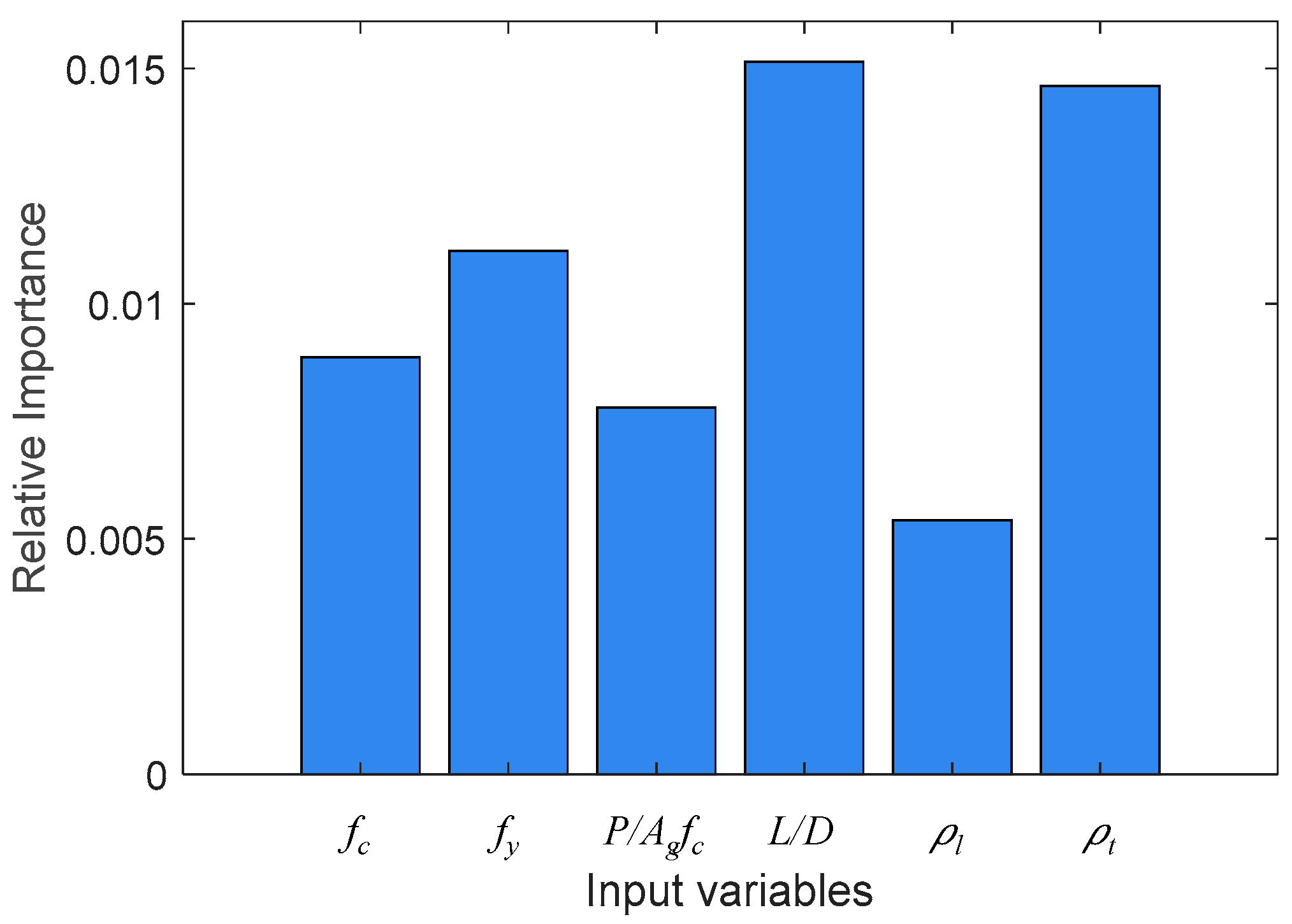
Figure 5 illustrates the relative importance of input variables. Here, each symbol represents concrete compressive strength (f_c), yield strength of reinforcement (f_y), axial force ratio (P/A_gf_c), aspect ratio (L/D), main reinforcement ratio (ρ_l), and shear reinforcement ratio (ρ_t). The factors influencing the failure type based on the training data were assessed through importance evaluation. Through the importance scores, one can understand the contribution of each variable to the model’s performance and assess the extent to which a particular variable plays a crucial role in predictions. The effect of confinement ratio related variables (e.g., height-to-depth aspect ratio, and shear reinforcement ratio) appears to be the highest, more significant than the influence of material properties. Additionally, it is observed that the main reinforcement ratio has a relatively lower impact compared to other input variables.

5. Demonstration of Machine Learning Model

To verify the ability of the machine learning model proposed in this study to predict the failure modes of RC columns, its results were compared with those obtained using the analytically determined shear demand curve and the shear capacity curve determined using equations provided in various standards. The shear demand curve was calculated using OpenSees [21], which utilizes a macroscopic approach based on fiber elements.

5.1. Shear Demand Curve

The shear demand curve is developed by modeling the flexural behavior of RC columns without considering shear failure, and a nonlinear static pushover analysis is performed. The RC column model reflects the inelastic behavior of the model materials, the effect of the confinement pressure resulting from transverse reinforcement, and bonding failure phenomena. To estimate the shear demand curves for flexure, shear, and flexure-shear failure, modeling methodologies were validated based on results of previous experimental studies [1,2,3].

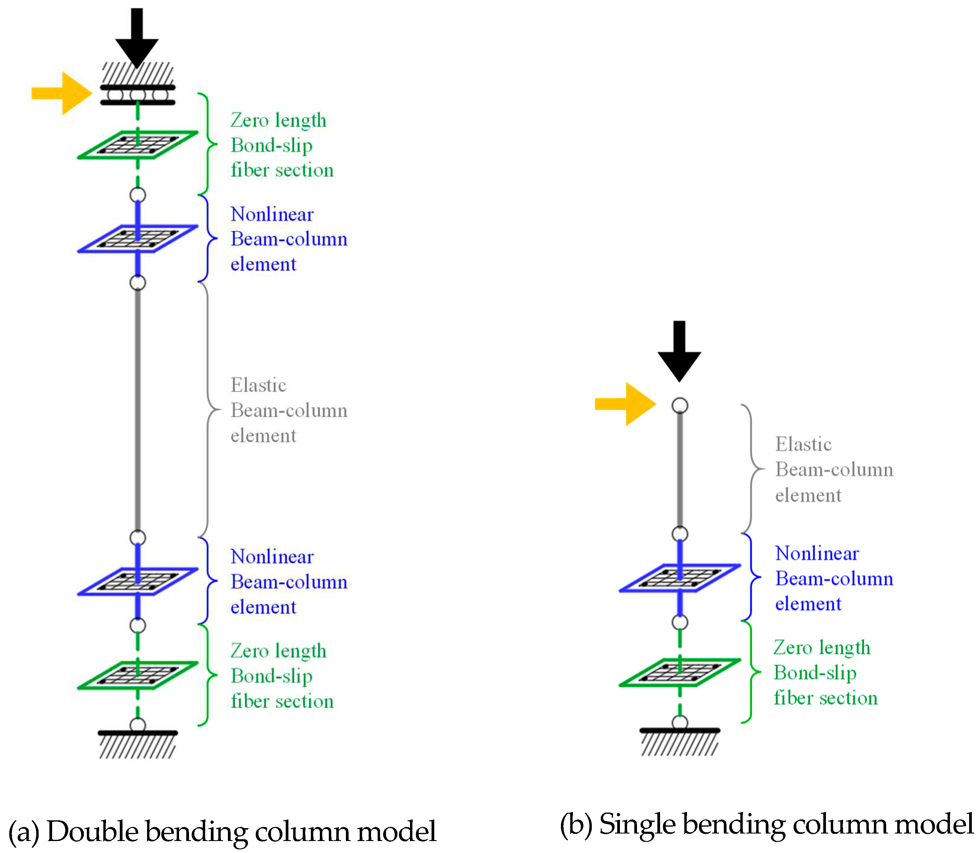
Figure 6 shows the details of the flexural behavior model. Columns were modeled using elastic beam-column elements, and plastic hinge regions were represented using displacement-based nonlinear beam-column elements with four integration points. The length of the plastic hinge region was set to the height of the column cross-section [22]. The Concrete02 material model was used to construct the fiber sections of the nonlinear beam-column elements. To account for the enhanced concrete compressive strength and ductility in areas confined by transverse reinforcement (confined concrete), the model proposed by Mander et al. [23] was utilized. The material model for the longitudinal reinforcement was the Steel02 material model, which allows for strain hardening.

Bonding failure in RC columns occurs when the bonding stress between the rebar and concrete exceeds the allowable bonding stress, leading to failure, which typically occurs at the top and bottom of the column where lap splices are located. In the flexure failure model, zero-length section elements were applied at the top and bottom of the column to incorporate bonding failure. The fiber sections of these zero-length section elements are identical to those in the column, but the material model is changed from a stress-strain relationship to a stress-slip relationship. The stress-slip relationship was applied using Equations (7) and (8), as presented by Sezen et al. [24].

{s l i p}_{y} = \frac{ϵ_{y} f_{y} ϕ_{c}}{8 u_{e}}

(7)

{S F}_{s l i p} = \frac{{s l i p}_{y}}{ϵ_{y}}

(8)

Here, slip_y is the yield slip for bonding failure (mm), ε_y is the yield strain of the longitudinal reinforcement, f_y is the yield stress of the longitudinal reinforcement (MPa), Φ_c is the diameter of the longitudinal reinforcement (mm), u_e is the elastic bonding stress (MPa), f_c is the concrete compressive strength (MPa), and SF_slip is the bonding failure variable. The strain in the rebar and concrete material models is multiplied by the bonding failure variable (SF_slip) to enable the use of the stress-slip relationship material model in the zero-length fiber sections.

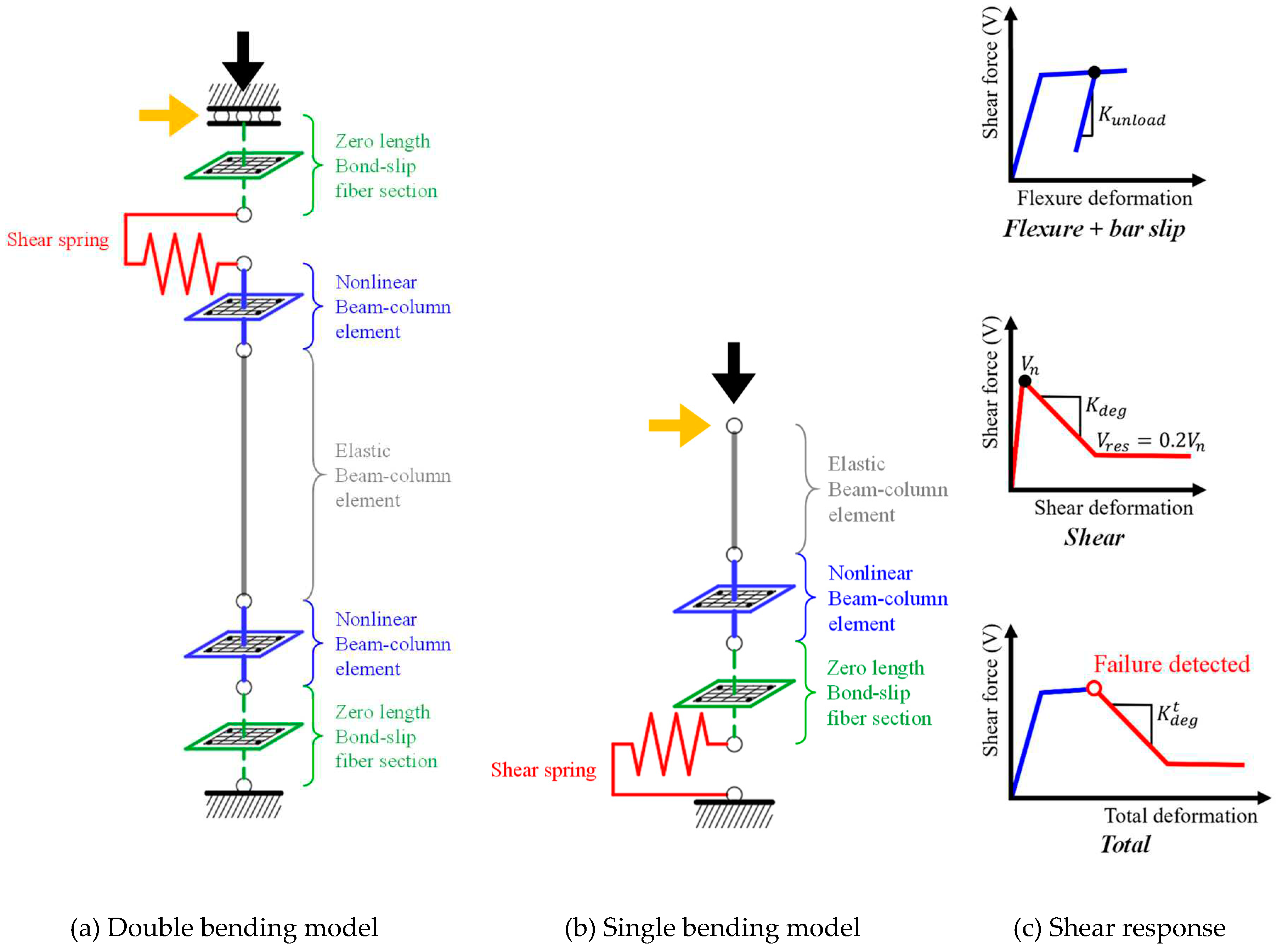
Figure 7 depicts the details of the model used to determine shear failure. The shear failure model is structured similarly to the flexure failure model, and the material model of the nonlinear beam-column elements using Concrete01 and hysteretic material models are used to accurately depict the characteristics of steel. Shear springs were applied as zero-length elements at the top or bottom of the model to represent shear failure behavior. The shear springs used the shear limit curve presented by Elwood [25] in the limit state material model. Shear failure, as shown in Figure 7(c), occurs when the member displaying flexural behavior reaches a certain shear strength (V_n), at which point the shear limit curve is applied, and shear failure behavior is shown. The shear strength (V_n) was calculated using Equation (9) from ASCE 41-23 [26].

V_{n} = k (\frac{A_{v} f_{y} d}{s} + λ (\frac{0.5 \sqrt{{f^{'}}_{c}}}{M / V d} \sqrt{1 + \frac{N_{u}}{0.5 \sqrt{{f^{'}}_{c}} A_{g}}}) 0.8 A_{g})

(9)

Here, k is 1.0 for a displacement ductility of <2, 0.7 for a displacement ductility of ≥6, and linearly progresses for 2 ≤ displacement ductility < 6; Av is the total cross-sectional area of the transverse reinforcement within spacing s (mm²); f_y is the designed yield strength of reinforcement (MPa); d is the effective depth of the column, which can be set as d = 0.8h (mm); s is spacing of the transverse reinforcement (mm); λ is 0.75 for lightweight concrete and 1 for normal concrete; f‘_c is the compressive strength of concrete; M/Vd is the maximum ratio of the column’s moment to shear force and effective depth under the design load, which ranges from 2 to 4; N_u is the axial load perpendicular to the cross-section, considered to be 0 for tensile loads (N); and Ag is the total cross-sectional area of the column (mm²).

Elwood [25] defined the reloading stiffness (K_deg) of the shear spring as a combination of the reloading stiffness during shear behavior (K^t_deg) and unloading stiffness during flexural behavior (K_unload), as per Equation (10). The reloading stiffness (K^t_deg) was determined using Equation (11), which was proposed by Baradaran [28].

\frac{1}{{K^{t}}_{d e g}} = \frac{1}{K_{u n l o a d}} + \frac{1}{K_{d e g}}

(10)

{K^{t}}_{d e g} = - 4.5 {(4.6 \frac{A_{v} f_{y v} d_{c}}{P s} + 1)}^{2} L

(11)

Here, A_v is the total cross-sectional area of the transverse reinforcement (mm²), f_yv is the designed yield strength of the transverse reinforcement (MPa), d_c is the central width of the column cross-section (mm), P is the axial load perpendicular to the column cross-section (N), s is the spacing of the transverse reinforcement (mm), and L is the total length of the column (mm). The residual shear strength (V_res) is applied as 80% of the shear strength (V_n).

The modeling methodology and results of past experimental studies [1,2,3] were compared using nonlinear static hysteresis analysis, and they are illustrated in Figure 8. A comparison of the flexure failure behavior and analysis results for the C3-1 specimen in Mo & Wang’s study [1] showed a gradual reduction in overall strength. In contrast, the shear failure behavior and analysis results of the 3SLH18 specimen obtained by Lynn et al. [2] showed a rapid reduction in strength and pinching effect. The comparison of the flexure-shear failure behavior and analysis results for Specimen 1 in the study by Sezen & Moehle [3] showed a gradual reduction in strength followed by a rapid decrease. Table 6 presents the initial stiffness, maximum strength, strength reduction rate, and energy dissipation capacity for each mode of failure in the experimental and analysis results. The error rate between the analysis and experimental results was calculated, and a good overall agreement was observed. The maximum error in the strength reduction rate occurred in Mo & Wang [1] for C3-1 at 16%. The strength reduction rate was calculated as the ratio of the residual shear strength (V_res) to the maximum shear strength (V_max). Adjusting the bonding failure variable (SF_slip) to match the initial stiffness led to reduced strength degradation, tuned through strain hardening. 3SLH18 in the study by Lynn et al. [2] and Specimen 1 in the study by Sezen & Moehle [3] showed the maximum errors in the energy dissipation rate at 14% and 22%, respectively. Energy is represented by the area of the hysteresis loop; the error in this case was relatively high due to the difference in the number of loops in the hysteresis loops of the experiments and analysis results.

5.2. Shear Capacity Curve

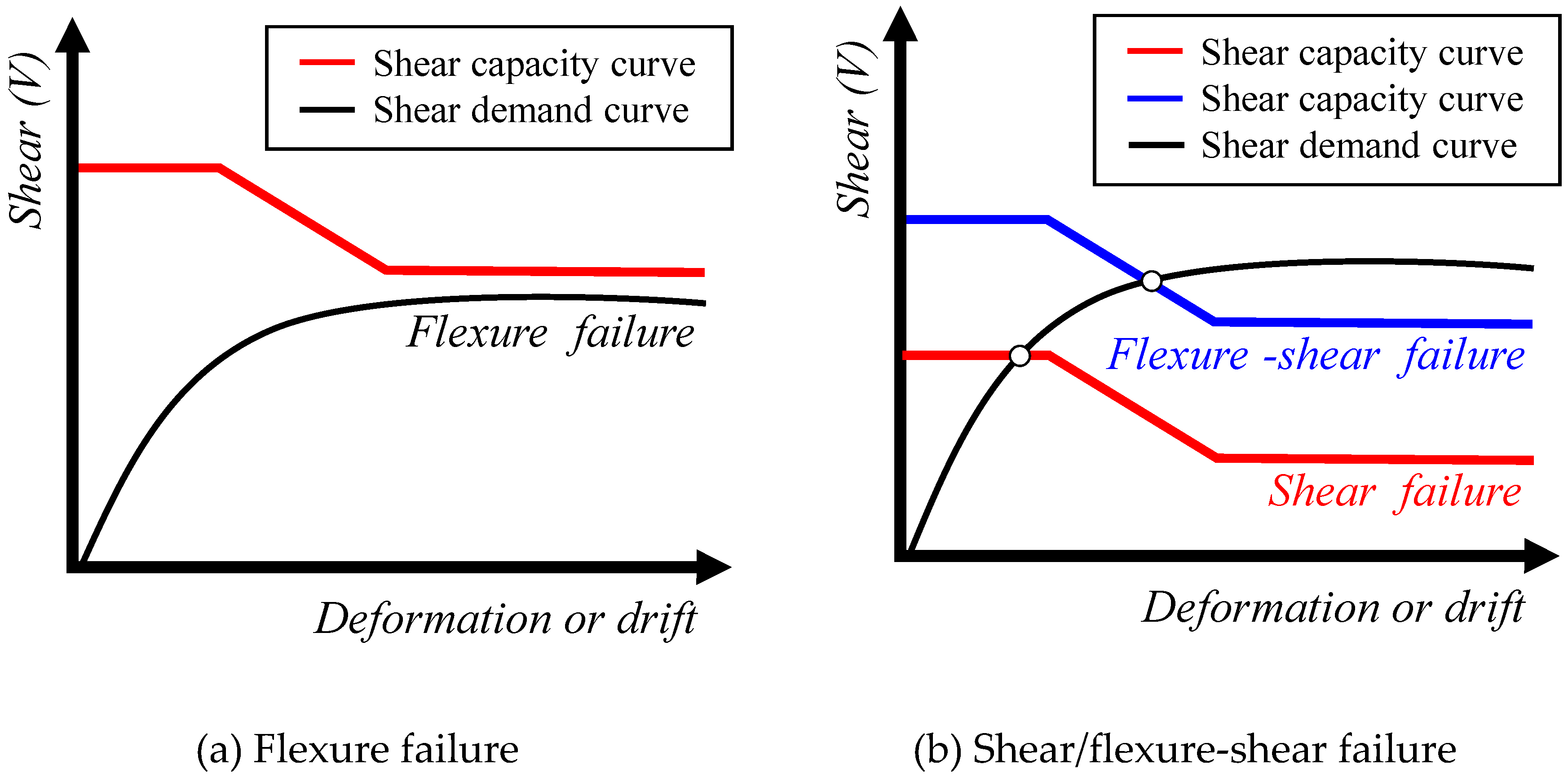
The shear capacity curve for RC columns was determined using Equation (9) from ASCE 41-23 [26,27,28], which accounts for a decrease in shear strength with increasing displacement ductility. The failure mode of RC columns can be determined based on the relationship between the analytically calculated shear demand curve and the shear capacity curve determined using the standard equation. The shear demand curve is derived from pushover analysis, and the yield displacement may be calculated. Based on the calculated yield displacement, the displacement ductility (k) is determined to derive the shear capacity curve. When comparing the shear demand curve with the shear capacity curve, as shown in Figure 9(a), if there is no intersection between the two curves, it is determined that flexure failure has occurred. In Figure 9(b), if there is an intersection between the shear demand and capacity curves, shear failure is indicated. If the intersection occurs before the yielding of the reinforcement, it is classified as shear failure; if it occurs after, it is classified as flexure-shear failure.

The relationship between the shear demand and shear capacity curves for previous experimental studies [1,2,3] used for validating the modeling methodology for each mode of failure is illustrated in Figure 10. For the C3-1 specimen in Mo & Wang’s study [1], the absence of an intersection between the shear demand and capacity curves indicates high ductility and flexure failure. The 3SLH18 specimen in Lynn et al.’s study [2] shows an early intersection between the two curves. Because the intersection occurs before the yielding of the reinforcement, it is classified as shear failure. Lastly, for Specimen 1 in Sezen & Moehle’s study [3], the intersection of the shear demand and capacity curves after the yielding of the reinforcement indicates flexure-shear failure.

5.3. Failure Mode Prediction

The method of determining the failure mode based on the relationship between the shear demand and shear capacity curves was compared with the results of the machine-learning-based model for failure mode prediction. Six key input variables were determined based on the structural details of previous experimental study specimens [1,2,3], as shown in Table 7. Applying these key input variables to the machine learning model, the C3-1 specimen in Mo & Wang’s study [1] was predicted to exhibit flexure failure, the 3SLH18 specimen in Lynn et al.’s study [2] was predicted to exhibit shear failure, and Specimen 1 in Sezen & Moehle’s study [3] was predicted to exhibit flexure-shear failure. The failure modes determined through the relationship between the shear demand and shear capacity curves agreed with the modes predicted using the machine-learning-based model. This demonstrates the capability of machine learning methods to accurately predict the failure modes of RC columns using only simple information.

6. Conclusion

This study proposed a machine learning model for rapidly predicting the failure modes of RC columns. To develop and validate the model for predicting column failure modes, four machine learning methods were employed using column data collected from past experiments and evaluated using classification model performance indicators. The following main conclusions were drawn.

(1): Overall, all considered machine learning methodologies accurately predicted the flexure failure mode. Since the high proportion of flexure failure modes in considered experimental dataset (flexure failure mode-72.4%, flexure-shear failure mode-14.8%, shear failure mode-12.7%), the flexure failure prediction was more accurate than other failure modes (flexure-shear and shear failure modes).
(2): Considering the average values of the classification model performance indicators, excluding accuracy, the RF model showed the highest performance level in precision, recall, F1-score, and AUC, suggesting that it accurately predicts the column failure modes.
(3): The RF model demonstrated the highest average values across all performance indicators used in accuracy validation and had the highest recall for shear failure modes. Therefore, the RF model, which provided conservative predictions based on simple structural details (i.e., the material strength, axial load ratio, aspect ratio, reinforcing details, etc.), was deemed the most rational for predicting failure modes before conducting experiments or analysis.
(4): The failure modes determined using the shear capacity and demand curves agreed with the failure modes predicted by the machine learning model for flexure, shear, and flexure-shear failures. This indicates that the machine-learning-based RC column failure-mode prediction model developed in this study can accurately and rapidly predict the failure modes of RC columns using only simple column information, without the need for experimental or analytical processes.

Acknowledgments

This work was supported by “Regional Innovation Strategy (RIS)” through the National Research Foundation of Korea (NRF) funded by the Ministry of Education(MOE)(2021RIS-003) and a grant(2022-MOIS63-003(RS-2022-ND641021)) of Cooperative Research Method and Safety Management Technology in National Disaster funded by Ministry of Interior and Safety (MOIS, Korea).

Conflicts of Interest

The authors declare that they have no known competing financial interests or personal relationships that could have appeared to influence the work reported in this paper.

References

Mo, Y.L. Wang, S.J. Seismic behavior of RC columns with various tie configurations. Journal of Structural Engineering 2000; 126: 1122-1130. [CrossRef]
Lynn, A.C. Moehle, J.P. Mahin, S.A. Holmes, W.T. Seismic evaluation of existing reinforced concrete building columns. Earthquake Spectra 1996; 12: 715-739. [CrossRef]
Sezen, H. Moehle, J.P. Seismic behavior of shear-critical reinforced concrete building columns. In Seventh US National Conference on Earthquake Engineering, Earthquake Engineering Research Institute, Boston, MA, 2002.
Zhu, L. Elwood, K.J. Haukaas, T. Classification and seismic safety evaluation of existing reinforced concrete columns. Journal of Structural Engineering 2007; 133: 1316-1330. [CrossRef]
Qi, Y.L. Han, X.L. Ji, J. Failure mode classification of reinforced concrete column using Fisher method. Journal of Central South University 2013; 20: 2863-2869. [CrossRef]
Naderpour, H. Mirrashid, M. Proposed soft computing models for moment capacity prediction of reinforced concrete columns. Soft Computing 2020; 24: 11715-11729. [CrossRef]
Mirrashid, M. Naderpour, H. Innovative computational intelligence-based model for vulnerability assessment of RC frames subject to seismic sequence. Journal of Structural Engineering 2021; 147: 04020350. [CrossRef]
Alibrandi, U. Alani, A.M. Ricciardi, G. A new sampling strategy for SVM-based response surface for structural reliability analysis. Probabilistic Engineering Mechanics 2015; 41: 1-12. [CrossRef]
Mangalathu, S. Jeon, J.S. Classification of failure mode and prediction of shear strength for reinforced concrete beam-column joints using machine learning techniques. Engineering Structures 2018; 160: 85-94. [CrossRef]
Naderpour, H. Mirrashid, M. Classification of failure modes in ductile and non-ductile concrete joints. Engineering Failure Analysis 2019; 103: 361-375. [CrossRef]
Alcantara, P.A. Imai, H. Failure mode classification of reinforced concrete columns by the analysis of the strain distribution in the main reinforcement. In Proceedings of the 12th world conference on earthquake engineering, Auckland, NZ, 2000.
Ying, M. Jin-Xin, G. Seismic failure modes and deformation capacity of reinforced concrete columns under cyclic loads. Periodica Polytechnica Civil Engineering 2018; 62: 80-91. [CrossRef]
Mangalathu, S. Hwang, S H. Jeon, J.S. Failure mode and effects analysis of RC members based on machine-learning-based SHapley Additive exPlanations (SHAP) approach. Engineering Structures 2020; 219: 110927. [CrossRef]
Feng, D.C. Liu, Z.T. Wang, X.D. Jiang, Z.M. Liang, S.X. Failure mode classification and bearing capacity prediction for reinforced concrete columns based on ensemble machine learning algorithm. Advanced Engineering Informatics 2020; 45: 101126. [CrossRef]
Berry, M. Parrish, M. Eberhard, M. PEER structural performance database user’s manual (version 1.0). University of California, Berkeley 2004.
Hiromichi, Y.O.S.H.I.K.A.W.A. Ductility and failure modes of single reinforced concrete columns. In JCI-C51E Seminar on Post-Peak Behavior of RC Structures subjected to Seismic Loads, 1999; Vol. 2:229-224.
Naderpour, H. Mirrashid, M. Parsa, P. Failure mode prediction of reinforced concrete columns using machine learning methods. Engineering Structures 2021; 248: 113263. [CrossRef]
Choi, J.S. Yang, W.J. Yi, W.H. Shear Strength Evaluation of Reinforced Concrete Columns 1: Variable Analysis for Code Method. Journal of the Architectural Institute of Korea (JAIK) 2017; 37: 687-688.
Bažant, Z.P. Kwon, Y. Failure of slender and stocky reinforced concrete columns: Tests of size effect. Materials and Structures 1994; 27: 79-90. [CrossRef]
Shi, Q. Ma, L. Wang, Q. Wang, B. Yang, K. Seismic performance of square concrete columns reinforced with grade 600 MPa longitudinal and transverse reinforcement steel under high axial load. In Structures, 2021; Vol. 32:1955-1970. [CrossRef]
McKenna, F. Scott, M.H. Fenves, G.L. Nonlinear finite-element analysis software architecture using object composition. Journal of Computing in Civil Engineering 2010; 24: 95-107. [CrossRef]
Berry, M.P. Lehman, D.E. Lowes, L.N. Lumped-plasticity models for performance simulation of bridge columns. ACI Structural Journal 2008; 105: 270.
Mander, J.B. Priestley, M.J. Park, R. Theoretical stress-strain model for confined concrete. Journal of structural engineering 1988; 114: 1804-1826. [CrossRef]
Sezen, H. Seismic behavior and modeling of reinforced concrete building columns. University of California, Berkeley 2002.
Elwood, K.J. Modelling failures in existing reinforced concrete columns. Canadian Journal of Civil Engineering 2004; 31: 846-859. [CrossRef]
American Society of Civil Engineers (ASCE). "Seismic evaluation and retrofit of existing buildings." American Society of Civil Engineers, 2023.
Elwood, K.J. Matamoros, A.B. Wallace, J.W. Lehman, D.E. Heintz, J.A. Mitchell, A.D. Moore, M.A. Valley, M.T. Lowes, L.N. Comartin, C.D. Moehle, J.P. Update to ASCE/SEI 41 concrete provisions. Earthquake Spectra 2007; 23: 493-523. [CrossRef]
Baradaran Shoraka, M. (Doctoral dissertation, University of British Columbia). Collapse assessment of concrete buildings: an application to non-ductile reinforced concrete moment frames, 2013.

Figure 1. Constituents of the reinforced concrete column database.

Figure 2. Frequency of input parameters.

Figure 3. Confusion matrix of each machine learning methodology for testing dataset.

Figure 4. ROC curve for all machnine learning models.

Figure 5. Relative importance of input variables.

Figure 6. Flexure-governed column modeling method.

Figure 7. Shear-governed column modeling method.

Figure 8. Validation of modeling method (experiment vs. simulation).

Figure 9. Traditional method predicting column failure mode.

Figure 10. Relationships between shear demand curve and shear capacity curve.

Table 1. The considered failure mode.

Failure Mode	Description
Flexure	Degradation occurred due to flexural deformation after yielding of the longitudinal reinforcement
Shear	Degradation (diagonal cracks) occurred due to shear distress before yielding of the longitudinal reinforcement
Flexure-shear	Degradation occurred after yielding of the longitudinal reinforcement but results from shear distress

Table 2. Summary of experimental database used in this research.

Parameter	Model range	Nominal	Extreme values
Parameter	Model range	Nominal	Minimum	Maximum
Concrete Compressive Strength (MPa)	13.10 to 48.30	34.11	13.10	48.30
Steel Yield Strength (MPa)	0 to 587.10	436.23	0	587.10
Axial Load Ratio	0.03 to 0.9	0.14	0.03	0.90
Slenderness ratio	1.12 to 8.67	2.43	1.12	8.67
Longitudinal Reinforcement Ratio	0.0009 to 0.0615	0.0073	0.0009	0.0615
Transverse Reinforcement Ratio	0.0068 to 0.0694	0.0174	0.0068	0.0694

Table 3. Summary of hyperparameters.

Model	Parameter	Value
ANN	Number of Layers	2
ANN	Activations	tanh
KNN	Number of Neighbors	3
KNN	Distance	cityblock
DT	Minimum of Leaf Size	1
DT	Maximum depth of the tree	177
RF	Method	AdaBoostM2
	Maximum depth of the tree	5
	Number of Learning Cycles	488
	Learning Rate	0.9274

Table 4. Confusion Matrix Concept.

Classification		Actual Class
Classification		Positive	Negative
Predict Class	Positive	TP (True Positive)	FP (False Positive)
Predict Class	Negative	FN (False Negative)	TN (True Negative)

Table 5. Results of performance measurement for classification models.

Measure		ANN	KNN	DT	RF
Accuracy		0.8820	0.9045	0.8632	0.8732
Precision	Flexure	0.9365	0.9833	0.9194	0.9355
	Shear	0.3333	0.3333	0.6667	0.7143
	Flexure-shear	0.8333	0.7778	0.5714	0.8333
	Overall	0.7010	0.6981	0.7192	0.8277
Recall	Flexure	1.0000	1.0000	0.9661	0.9831
	Shear	0.5000	0.5000	0.6667	0.8333
	Flexure-shear	0.4167	0.5833	0.4000	0.5000
	Overall	0.6389	0.6944	0.6776	0.7721
F1-Score	Flexure	0.9672	0.9916	0.9421	0.9587
	Shear	0.1721	0.1681	0.4714	0.6205
	Flexure-shear	0.3586	0.4575	0.2425	0.4344
	Overall	0.4993	0.5391	0.5520	0.6712
AUC	Flexure	0.9958	0.9688	0.9619	0.9905
	Shear	0.9648	0.7218	0.9275	0.9517
	Flexure-shear	0.8862	0.7758	0.9385	0.9185
	Overall	0.9489	0.8221	0.9426	0.9536

Table 6. Comparison between experiment and simulation.

Specimens		Initial Stiffness (kN/mm)	Maximum Strength (kN)	Strength Reduction Ratio	Energy Dissipation (kN-m)
C3-1 (Mo & Wang 2000)	Experiment	16	235	0.70	818.2
	Simulation	18	229	0.81	751.9
	Error(%)	13%	3%	16%	8%
3SLH18 (Lynn et al. 1996)	Experiment	14	270	0.26	268.7
	Simulation	15	260	0.27	306.9
	Error(%)	7%	4%	4%	14%
Specimen 1 (Sezen et al. 2006)	Experiment	19	303	0.22	251.3
	Simulation	20	309	0.25	307.4
	Error(%)	5%	2%	14%	22%

Table 7. Predicted Results of Classification Model.

Specimens	fc (MPa)	fy (MPa)	P/Agfc	L/D	ρl	ρt	Predicted Failure Mode
C3-1 (Mo & Wang 2000)	26.4	497	0.107	3.93	0.0214	0.0126	Flexure
3SLH18 (Lynn et al. 1996)	26.9	331	0.089	3.65	0.0303	0.0015	Shear
Specimen 1 (Sezen et al. 2006)	21.1	434.4	0.151	3.90	0.0247	0.004	Flexure-shear

Disclaimer/Publisher’s Note: The statements, opinions and data contained in all publications are solely those of the individual author(s) and contributor(s) and not of MDPI and/or the editor(s). MDPI and/or the editor(s) disclaim responsibility for any injury to people or property resulting from any ideas, methods, instructions or products referred to in the content.

© 2024 by the authors. Licensee MDPI, Basel, Switzerland. This article is an open access article distributed under the terms and conditions of the Creative Commons Attribution (CC BY) license (http://creativecommons.org/licenses/by/4.0/).

Copyright: This open access article is published under a Creative Commons CC BY 4.0 license, which permit the free download, distribution, and reuse, provided that the author and preprint are cited in any reuse.

MDPI Initiatives

Important Links

Choose an area of interest and we will send you notifications of new preprints at your preferred frequency.

Disclaimer