Using Basic Quantum Circuits to Simulate 1D Ising Model

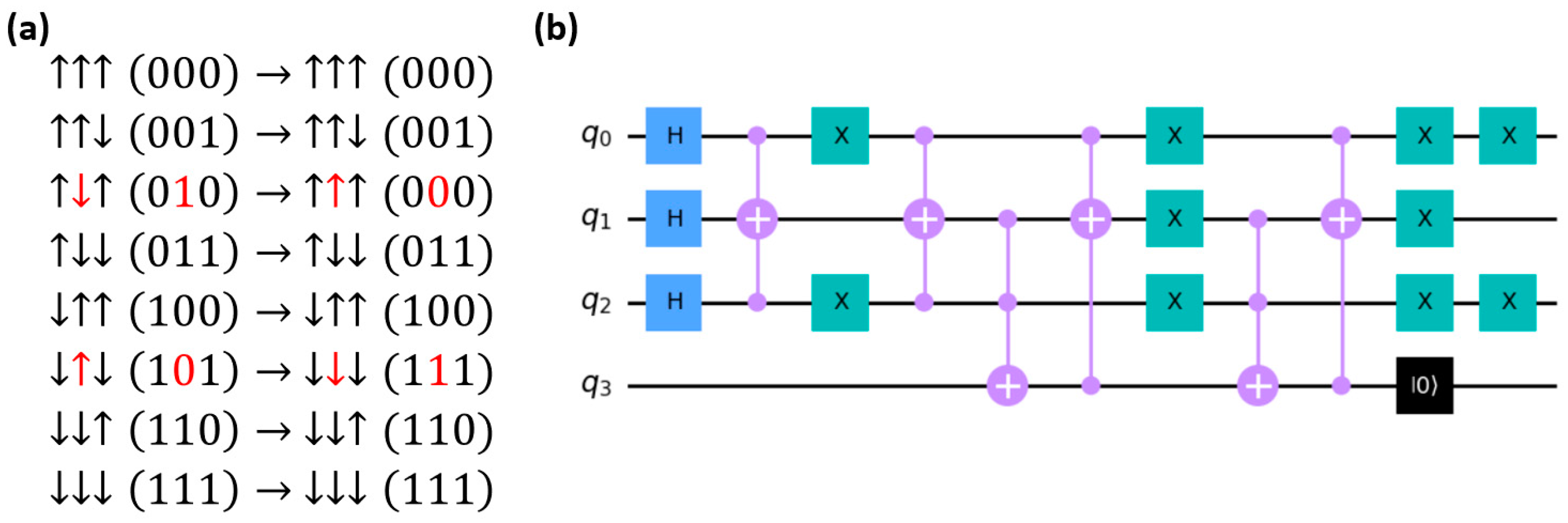
As have discussed in the previous section, we know that the final magnetization of the 1D Ising model is determined by the three free parameters $J, \beta$ and $h$. In order to use quantum computing to simulate the system, we need to encode this information into the quantum circuits. For the exchange interaction with the nearest neighbor, we considered all eight possibilities for three qubits. We used the middle qubit as a reference to observe how the exchange interaction evolves the state, as illustrated in Figure 1a. It is observed that the middle spin flips only when the two nearest neighbors are identical but opposite to the middle reference spin. This suggests the use of the CCX gate to ensure that both sides are the same while controlling the middle state.

However, relying solely on the CCX gate is insufficient, as it would incorrectly flip states where all three spins are identical, such as in the $\uparrow \uparrow \uparrow$ and $\downarrow \downarrow \downarrow$ cases. To circumvent this, we employ an ancillary qubit to determine whether all three spins are identical. If they are, the middle spin undergoes an additional flip to rectify the erroneous flip. This correction does not interfere with cases like $\uparrow \downarrow \uparrow$ and $\downarrow \uparrow \downarrow$, where the flip occurs only if all bits are the same. The final step involves resetting the ancillary qubit for reuse with the next spin. By looping this process across the entire 1D spin chain, we can effectively simulate the exchange interaction. Subsequent to this calculation, a random number generator produces a number between 0 and 1. In a manner akin to the classical Monte Carlo method, if the random number is smaller than $e^{-\beta }$, the corresponding spin is flipped. This approach is chosen because we assumed the exchange interaction, $J$, to be 1.

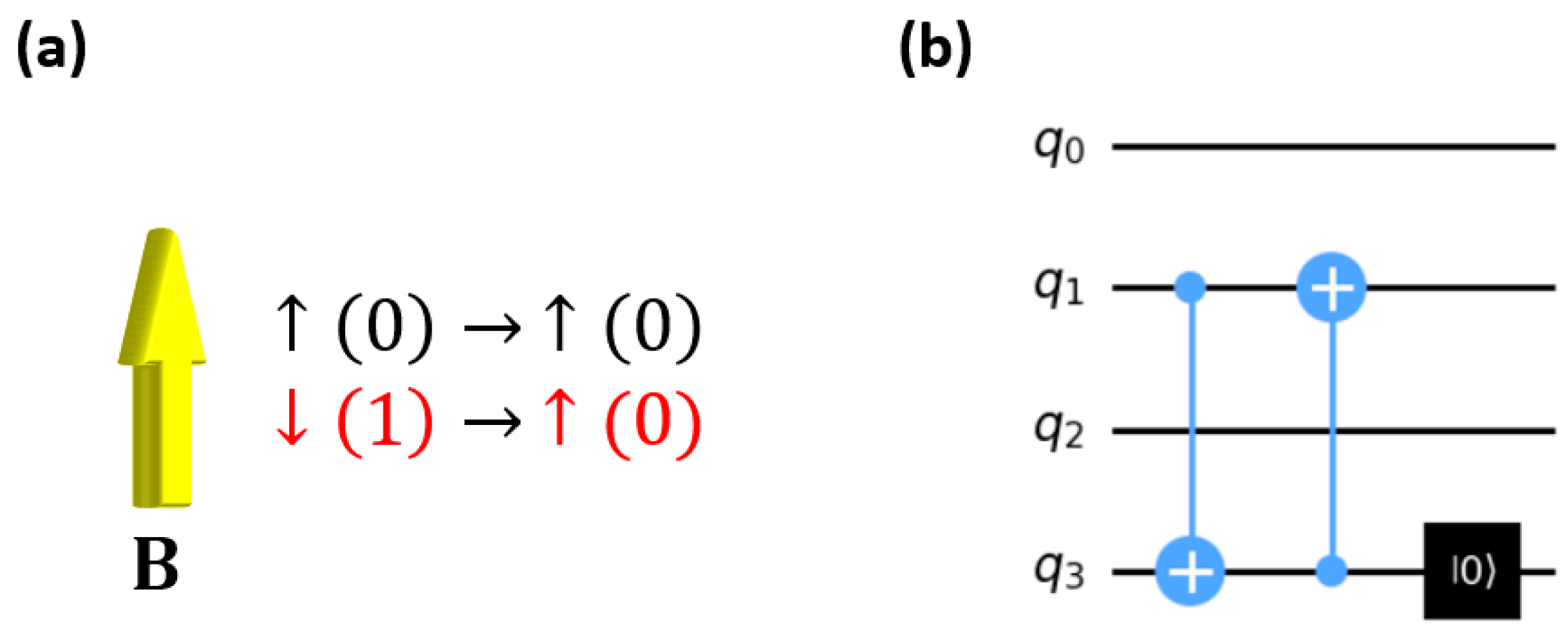
The spin alignment caused by the external magnetic field is also a key part in the Ising model. To make the problem easy to solve, we assume that the direction of the magnetic field is the same as what the $|0$〉 directs. Consequently, our objective is to implement a quantum operation that flips the state from $|1$〉 to $|0$〉, emulating the alignment of a spin with the magnetic field. The quantum circuit representing this magnetic field alignment is depicted in Figure 2a. In this setup, the flip operation is selectively applied only when the qubit state is $|1$〉.

To achieve this selective flipping, we employ an ancillary qubit in conjunction with a combination of controlled-NOT (CNOT) and controlled rotation gates. This configuration ensures that only the $|1$〉 state is flipped to $|0$〉, while $|0$〉 remains unaffected. Additionally, the ancillary qubit is reset after each operation to be reused for subsequent spins. It's important to note that the thermal effects are also taken into account in this simulation. Similar to what we have discussed above, if the random number is smaller than $e^{-\beta h}$, the corresponding spin will be flipped due to the thermal effect.

Our simulation begins by examining an 8-spin Ising system in the absence of an external magnetic field. We opted for an 8-spin system as a balance between computational feasibility and the need for a sufficiently large system to align with the approximations inherent in the rigorous solutions. We define the step or the time in this simulation as the loop number of every spin being exposed to the quantum gates. As long as all the spins are being executed by the quantum gates, we assume the step or the time will add one more. To ensure statistical significance in line with the law of large numbers, we executed 100,000 shots for each configuration. On average, each data point takes about several hours to get. 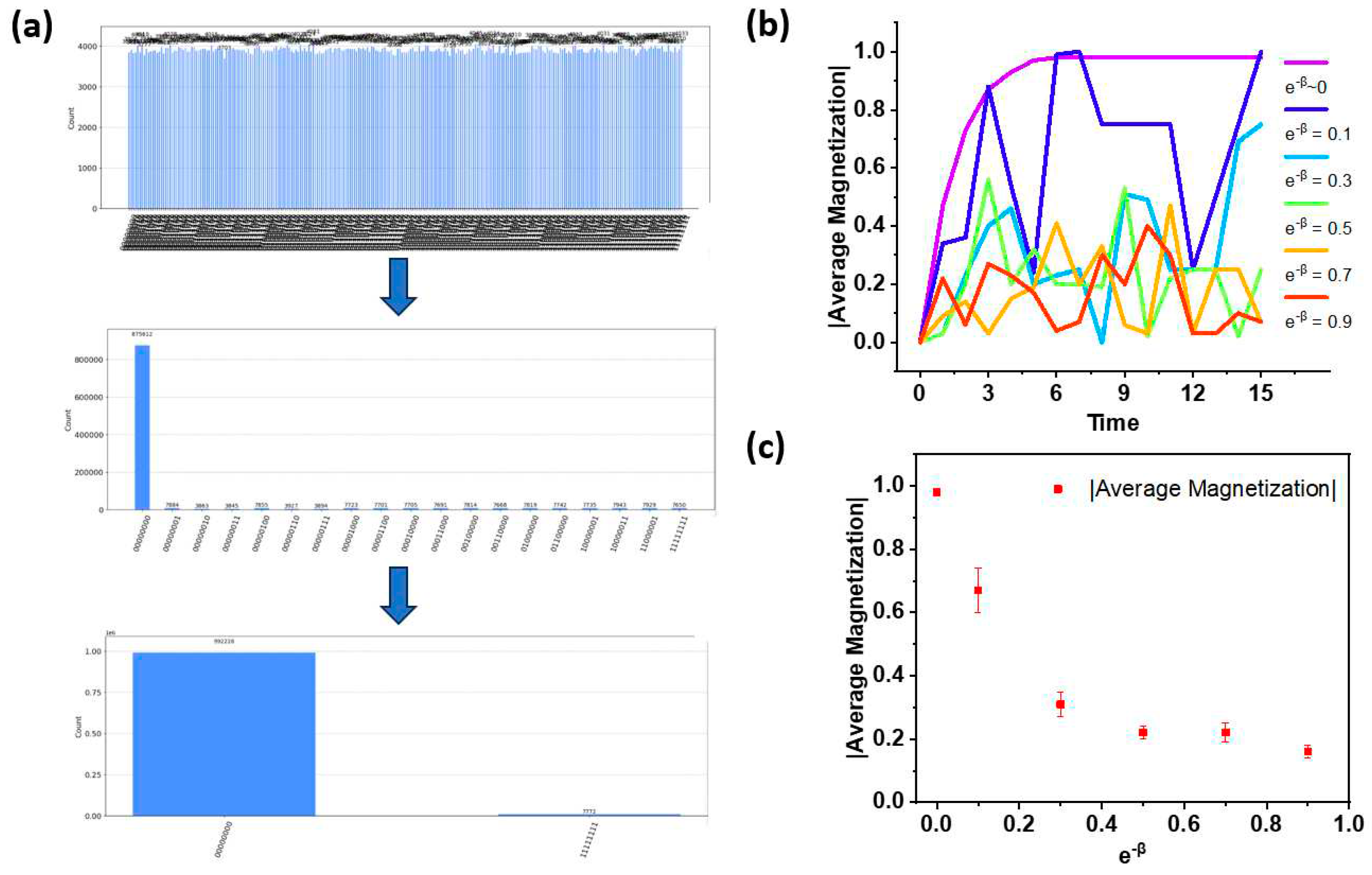Figure 3(a) shows how the system evolves under the temperature that is very close to zero. As we can see, the system starts with the mixed states of all the possible states with equal possibilities. And after several steps, some possibilities disappears and some possible states are enhanced. And after long enough steps, the stable states finally appear with all the spin direct in the same direction, which agrees well with the phase transition at zero temperature.

The temperature dependent results, as depicted in Figure 3(b), cover a range from near absolute zero to approximately $\frac{10}{k}~\frac{10J}{k}$. From our analysis, several key features emerged. The first is the zero-temperature ferromagnetism. Consistent with the rigorous solution, we observed that the system exhibits ferromagnetic behavior (where the static magnetization reaches 1) exclusively at zero temperature. This aligns with the theoretical understanding that, in the absence of a magnetic field, the Ising model does not exhibit ferromagnetic order at finite temperatures. The second feature is that as the temperature increases, the average magnetization approaches zero, reverting to the initial state of the system. As displayed in Figure 3(c), we statistically show the absolute value of the average magnetization and its variation based on the last 10 steps of simulation. This trend is in line with physical intuition: higher thermal fluctuations disrupt the ability of spins to maintain macroscopic magnetization. Thus, at elevated temperatures, the system tends toward a disordered state, characterized by reduced magnetization. These simulation results underscore the critical role of temperature in influencing the magnetic properties of the Ising model and agree well with the rigorous solution, further confirming our quantum circuits are correct.

Next, we take the external magnetic field into account. Based on the rigorous solutions [5], as illustrated in the Supplementary Information, the magnetization $m_{RS}$ is described by the following formula:

We apply this formula to the 8-spin Ising model previously discussed. The simulation evolves over 15 steps, with statistics—average and variation—computed from the last ten steps to represent the average magnetization of the system. The magnetization under different temperatures and magnetic fields are shown in Figure 4. A notable uncertainty in our results can be attributed to the limited number of spins in the simulation. Operating with only 8 spins, a single spin flip within the ferromagnetic phase can cause the average magnetization to drop from 1 to 0.75, significantly impacting the outcome. Furthermore, our simulation results are consistently lower than theoretical predictions, which may be due to insufficient simulation steps. Certain data points suggest the need for extended simulation durations to allow the system to reach equilibrium. This extended time would likely lead to more accurate simulation results that are closer to theoretical expectations.

In this work, we have successfully utilized QISKIT to construct a simulation of the 1D Ising model using basic quantum gates. This simulation is accessible to novices in the field due to its reliance on fundamental quantum gates, and it is designed to be operable on standard personal computers, bypassing the need for specialized computational resources. Our approach initializes the system in a superposition of all possible mixed states, employing quantum gates to emulate the interactions between spins and between spins and an external field. This method presents a more instinctive and straightforward way of observing the system's evolution compared to earlier techniques. Our findings confirm the absence of a phase transition at finite temperatures within the 1D Ising model, providing a quantum computational perspective to a well-established concept in statistical mechanics. Furthermore, we demonstrate the potential of our program to be extended beyond the Ising model. By substituting the X gates with rotation gates of a specified angle, we can adapt the simulation to handle the XY model, allowing for a continuous range of spin states between 1 and -1. This versatility highlights the promising applications of quantum computing in advancing the study of complex physics systems and enriching our understanding of critical phenomena in statistical physics.

References

- Ising, E. Beitrag zur Theorie des Ferromagnetismus. Z. Physik 1925, 31, 253–258. [Google Scholar] [CrossRef]
- Brush, S.G. History of the Lenz-Ising Model. Rev. Mod. Phys. 1967, 39, 883–893. [Google Scholar] [CrossRef]
- Kaye, P.; Laflamme, R.; Mosca, M. An introduction to quantum computing. (Oxford University Press, 2007).
- Cervera-Lierta, A. Exact Ising model simulation on a quantum computer. Quantum 2018, 2, 114. [Google Scholar] [CrossRef]
- Pathria, R.K.; et al. Statistical Mechanics. 2011. [Google Scholar]