Submitted:
09 January 2024
Posted:
11 January 2024
You are already at the latest version
Abstract
Remotely sensed data acquired by multispectral sensors can be used to monitor soil moisture (SM) across a larger land area than in situ monitoring alone. Although there have been wide-ranging applications of remote sensing tools in SM estimation on many ecosystems, there is a limited understanding of their accuracy in restored wetlands. The objective of this study was to examine the potential of remotely sensed data from Landsat-9, Sentinel-1A SAR, and Blackswift E2 Uncrewed Aircraft Systems (UAS) in predicting SM in a restored wetland complex in the Gunnison Basin of Colorado. We tested two response variables, gravimetric SM and volumetric SM, to determine which indicator of SM was better predicted with remotely sensed data. We also tested the accuracy of remotely sensed data in predicting SM at different soil depths. Overall, satellite and UAS indices predicted gravimetric SM better than volumetric SM. The Normalized Difference Red Edge (NDRE) index from Blackswift E2 UAS had the best prediction of GSM at the depth of 0 to 5 cm (R2 = 0.86, RMSE = 7.41). Results from the study provide information on the accuracy of remotely sensed data for SM monitoring on restored wetlands.
Keywords:
Gravimetric soil moisture
; Multispectral images
; Satellite images
; Uncrewed aircraft systems
; Vegetation indices
; Volumetric soil moisture
; Wetland restoration
1. Introduction
Historically, engaging in ground-based soil moisture (SM) measurement has been considered to yield the most accurate results [1]. However, ground-based SM measurements are often limited by cost, time, associated destructive mechanisms, and the inability to provide information for a large area [2]. Owing to these limitations, it is challenging to measure SM at the landscape level. The use of remotely sensed data from multispectral sensor systems might be effective at measuring SM at a larger spatial scale, particularly on restored landscapes. Landscape restoration is widespread and expensive, and developing new monitoring strategies could allow us to track the effects of these large-scale interventions more effectively; however, more research is needed to determine which sensors and indices are most informative for this purpose.
Remote-sensing platforms such as satellites can be equipped with sensors that make them suitable for estimating SM [3] on a larger spatial scale, within short time intervals, and at low costs. Some of these sensors include the active microwave sensors that estimate SM by sending a pulse and analyzing the soil-reflected signals. A typical example of active microwave sensors is the Synthetic Aperture RADAR (SAR) which is a well-adopted technique for the estimation of SM [4]. Some other sensors include the passive sensors on satellites such as LANDSAT, SMAP, and MODIS that estimate SM by collecting signals emitted by the soil and vegetation. In previous studies, indices such as the Normalized Difference Vegetation Index (NDVI) analyzed from these satellite images showed the potential of estimating SM with high correlation values [5].
However, images acquired from these traditional remote sensing techniques are generally limited in their spatial resolution, and resampling or down-scaling must often be performed to improve their applicability. In addition, there is a limitation of revisit time (temporal resolution) associated with some of these traditional satellite platforms, limiting the accuracy of the estimated SM at the field scale. The emergence and development of uncrewed aircraft systems (UAS) might provide solutions to the limitations of traditional remote sensing techniques [6]. UAS technology allows collection of ultra-high resolution remote sensing imagery. UAS remote sensing systems provide high-resolution data at the field scale and can be easily deployed, reducing the limitations of revisit time and operating costs [7]. UAS has been used in a series of ecological studies to estimate SM through the development of algorithms and integration of indices derived from multispectral and thermal images [8]. Due to the advancement of remote sensing techniques in ecosystem monitoring, it is assumed that these techniques might proffer solutions to the challenges associated with ground-based SM monitoring.
Studies have shown the wide application and usefulness of remote sensing techniques in different ecosystems. For instance, remotely sensed data has been used in agricultural ecosystems for irrigation management [9] and crop yield estimation [10]. It has also been used in forest and wetland ecosystems to characterize forest structure [11] and for wetland classification [12]. Although remote sensing techniques have been applied on restored wetlands, many of the applications only centers around the monitoring of vegetation structures [13,14,15,16], with little to no applications on SM measurements. Also, while researchers have successfully used a variety of methods, incorporating satellite data from a single sensor, a combination of satellite sensors, and UAS images to estimate SM, only few have compared the accuracy of both satellite and UAS images for estimating SM.
Therefore, this study was targeted toward investigating the potential and accuracy of remotely sensed (RS) data in estimating SM on a restored wet meadow site in the Gunnison Basin, Colorado. Specifically, we identified three research objectives which include determining (1) the potential and accuracy of satellite images in estimating SM at different depths, (2) the potential and accuracy of the multispectral sensors on the Blackswift S2 UAS in estimating SM at different depths, and (3) the measure of SM i.e., gravimetric soil moisture (GSM) or volumetric soil moisture (VSM) that can be better predicted by satellite and UAV indices. To answer our questions, we developed a procedure that combined field survey techniques, satellite and UAS images, and linear regression models for SM estimation on the restored wetland ecosystem. Established models across depths and different RS data types were validated to determine accuracy. The results obtained from this study provide vital information on how RS data can be effectively used to monitor SM in restored wet meadows.
2. Materials and Methods
2.1. Study Site
This research was conducted at the Sapinero Mesa watershed in the Upper Gunnison Basin (UGB) of Western Colorado. The center of the watershed is at 38.367598N and 107.237498W, at an elevation of 2,438.4 to 2,743.2 m. The watershed is managed by the Bureau of Land Management (BLM). The climate in the UGB ranges from cool to cold and dry to moist, with a mean precipitation of 30.9 mm in summer and 19.6 mm in winter. The average maximum and minimum temperature in summer are 24.6 °C and 4.6 °C, and -2.4 °C and -19.4 °C in winter between 2007 - 2019. The mean snowfall in winter for this area is 254 mm [17]. The mean rainfall in the month (July) prior to data collection was 46.74 mm and the mean rainfall in the months (August and September) data were collected was 18.80 mm and 10.16 mm.
At the bottom of the basin is the Sagebrush Steppe which serves as a habitat for the Gunnison Sage-grouse (Centrocercus minimus). The parental material of the soil types of riparian and wetlands in the UGB is Rhyolite and the typical soil profiles range from H1 – H4. The H1 is the loam which ranges from 0 – 0.25 m and the H2 represents the clay loam with a range of 0.25 – 0.38 m. The H3 and H4 both represent the gravelly clay and gravelly clay loam with ranges of 0.38 – 1.19 m and 1.19 – 1.52 m respectively. The soil in Sapinero Mesa is well-drained [18].
Restoration activities began at the Sapinero Mesa watershed in 2017 to enhance ecosystem resilience against the compounding effects of climate-induced drought [19]. The Gunnison Climate Working Group (GCWG) collaborated on the landscape-scale restoration project, which was centered on species and habitats that were recognized as threatened or degraded. For the restoration process, a series of techniques and structures which helped to slow and disperse water within the ephemeral and perennial stream systems were used [20]. The structures allowed water to gently seep in, hold and disseminate water, capture sediments, and spread out mesic and wetland plant species.
Within the Sapinero watershed, we selected an area of 0.5 km2 as the footprint for obtaining satellite data, flying the UAS, and collecting ground-based SM data (Figure 1). We selected this area size because of the need to reflect the spatial resolution of the RS techniques used and because of the flight length limitations of the Blackswift UAS used. We also selected this study area size to capture a range of SM variability within the study area. As such, both areas that were restored by the installation of structures, and the adjacent sagebrush ecosystem were included in the study area.
2.2. Landsat-9 Imagery and Sentinel-1A Imagery Data
The satellite data used for this study were obtained from images of two satellites: Landsat-9 and Sentinel-1A.
The LANDSAT-9 data from the OLI-2 instruments (spatial resolutions of 30 m) were acquired on the 1st of August and 9th of September 2022 and were downloaded as Level 2 products from the United States Geological Survey’s website http://glovis.usgs.gov/ (Table 1). From the Landsat-9 data, we analyzed the Normalized Shortwave-Infrared Difference SM Index (NSDSI2) and Normalized Difference Vegetation Index (NDVI) for the prediction of SM, and the calculation of these indices were carried out in the Raster Calculator tool of ArcGIS Pro (ESRI, version 3.0.3).
The Sentinel-1A SAR imagery acquired on the 28th of July and the 9th of September 2022 was used for this study. The data was downloaded from the Alaska Satellite Facility (ASF) website https://asf.alaska.edu/data-sets/sar-data-sets/sentinel-1/sentinel-1-data-and-imagery/. Sentinel-1 SAR images with a spatial resolution of 10 m are usually acquired in both singular (HH or VV) and dual polarization (HH+HV or VV+VH) within 12 days of the repeat cycle. For this study, only the VV polarization data was used to determine the Backscattering coefficient (dB), and the process was carried out in the Sentinel Application (SNAP) software. The VH polarization data was not used because it has a limited potential for the estimation of SM because of its high sensitivity to volume scattering, which depends strongly on vegetation properties [21]. The Sentinel-1A acquisition mode used for this study was the Interferometric Wide Swath (IW) which is available in both single and dual polarization and used for land monitoring. More information about the specifications of the data used is presented in Table 1.
2.3. UAS Imagery Data
The UAS data used for this study were acquired with Blackswift E2 UAS, an American-made autonomous inspection drone [22]. A MicaSense Altum camera with five multispectral bands (Red, Blue, Green, Near-infrared, Red-edge) was mounted on the E2 UAS to capture images from which indices were analyzed (Table 2). The acquisition of UAS data was only carried out on September 9, 2022, and did not take place in August because of unfavorable weather conditions. The image processing of the UAS data and analyses was carried out by Black Swift Technologies LLC using the Solvi software (https://solvi.ag/ ). Altogether, five vegetation indices were analyzed from UAS images for the estimation of SM.
2.4. Ground-based Data Collection and Soil Moisture Determination
To test the effectiveness of using RS data to estimate SM, we collected information on SM with two field-generated variables: VSM collected on-site, and GSM generated in the lab from field-collected soil samples. The field sampling procedure of SM was done at a resolution of 30 m and all other satellite images were resampled to the same resolution to facilitate proper data comparisons. The field sample design was carried out by clipping a Landsat image (30 m resolution) to the 0.5 km2 study area. Landsat pixels were converted to center points. Transects that ran perpendicular to the stream were generated by connecting 10 adjacent pixel center points. From all transects, five transects were randomly selected, consisting of a total of 50 sampling points (5 transects x 10 points = 50 points). This systematic random sampling method was adopted to ensure that we captured a range of SM values and to increase the accessibility to sampling plots.
At each sampling point, the percent VSM was measured directly (single measurement per point) in the field using a Time Domain Reflectometry SM probe (FieldScout TDR 300 Soil Moisture meter, Spectrum Technologies, Aurora, IL, USA; with 7.6 cm and 20 cm rods). Soil samples were also collected at the center of each pixel along the transect using a soil core with a hammer attachment. Collected soil samples were brought in airtight containers to the lab for analysis.
Data from the field was gathered twice, at different times. The first round of ground-based data collection took place on August 1 and 2, 2022. The original plan called for collecting soil samples and SM data from a depth of 0 to 10 cm and from 0 to 20 cm at each of the 50 points. Due to the rockiness of the study site, the collection of soil samples and the measuring of VSM with the probe at the depth of 0 to 20 cm were only possible at 48 and 49 points, respectively. However, the collection of soil samples and VSM at the depths of 0 to 10 cm and 0 to 7.6 cm was possible at each of the 50 points. As a result, a total of 98 soil samples were collected from the field and a total of 99 VSM data were measured in the field.
On September 9th, 2022, the second round of data collection took place. While soil samples were taken at depths of 0 to 5 cm and 0 to 10 cm, VSM data was collected at the depth of 0 to 7.6 cm only. Due to unfavorable weather, the UAS was only able to fly over a portion of the 0.5 km2 area, sampling only 30 points. Therefore, for this second data collection period, all data were collected from only 30 of the original 50 points. A total of 60 soil samples from the field were gathered and processed in the lab for the second ground-based data collection (Table 3).
Gravimetric SM (g soil per g water) was measured in the laboratory from field-moist extracted soil cores, sieved to 2 mm [23]. A subsample (5 – 10 g) of soil was weighed, then placed in the hot-air oven and dried at 105 °C for a minimum of 72 hours. After drying, the samples were weighed again to obtain a dry weight, and SM was estimated using the following equation:
Where Mw is the mass of water and Ms is the mass of dry soil,
Mw = (weight of wet soil) – (weight of oven-dry soil)
Ms = (weight of oven-dry soil)
2.5. Satellite Images Indices
To estimate the SM of the study area from the Landsat-9 indices, a corresponding pixel value for each sampling point was extracted in the ArcGIS Pro software. This was done using the “extract multi-values to points” tool. The extracted values were used as independent (predictor) variables in linear regression analyses to estimate SM. Descriptions of the indices analyzed from Landsat-9 images are specified below:
2.5.1. Normalized Shortwave-infrared Difference Soil Moisture Index (NSDSI2)
The Normalized Shortwave-infrared difference SM index was analyzed from Landsat-9 images. The difference in reflection values caused by differences in water absorption rates in shortwave infrared bands was used to calculate this index [24]. Using Bands 6 (SWIR1) and 7 (SWIR2) of Landsat-9 data, the NSDSI2 was generated.
2.5.2. Normalized Difference Vegetation Index (NDVI)
The Normalized Difference Vegetation index shows the difference between vegetation reflectance in the visible and near-infrared bands and the soil [25]. To analyze the Normalized Difference vegetation index, Band 5 (NIR) and Band 4 (RED) of Landsat-9 data were used.
2.5.3. Backscattering Coefficient (dB)
The backscattering coefficient was analyzed from Sentinel-1A data. The European Space Agency (ESA) provided steps to be performed with open-source tools of Sentinel Application Platform (SNAP) software for determining the backscattering coefficient (σ0). The steps include applying orbit file, thermal noise removal, border noise removal, radiometric calibration, speckle filtering, range doppler terrain correction, and Conversion to dB (backscattering coefficient) [26]. The graphic builder in SNAP was used to build a model (Figure 2) with which dB was analyzed.
2.6. UAS Multispectral Indices
Five vegetation indices were analyzed from the Blackswift E2 UAS imagery and include NDVI (see eq 2), ENDVI, NDRE, GRVI, and GLI. The indices were analyzed using the five spectral wavelength bands (Table 2; Supplemental Table 1) of the MicaSense Altum sensor. To extract index values, a buffer of 30 m by 30 m (LANDSAT resolution) was created around each sampling point and the mean value of all pixels within the buffer was calculated in ArcGIS pro. The calculated index values were used as independent variables to predict SM. More information about the different UAS indices is given below.
2.6.1. Enhanced Normalized Difference Vegetation Index (ENDVI)
To get a more sensitive result than NDVI, the Enhanced Difference Vegetation Index compares the NIR, Green, and blue bands from the E2 UAS. A plant's presence and health can be determined using the index [27].
2.6.2. Normalized Difference Red Edge Index (NDRE)
The normalized difference red edge index was analyzed from the near-infrared and red-edge bands of the E2 UAS. NDRE is sensitive to soil background effects, variations in leaf area, and leaf chlorophyll concentration. Higher NDRE values than lower ones correspond to higher leaf chlorophyll concentration levels. Typically, healthy plants have the greatest NDRE values, whereas unhealthy plants have intermediate values [28].
2.6.3. Green-Red Vegetation Index (GRVI)
2.6.4. Green Leaf Index (GLI)
The relationship between the reflectance in the green channel in comparison to the other two visible light channels (red and blue) is represented by the greenness index, also known as the green leaf index [31].
2.7. Ground-based Soil Moisture Data
Using a univariate approach, ground-based data outside 1.5 * IQR (Inter Quartile Range) i.e., outliers were determined. Three and eight individual sampling measurements of GSM were recognized as outliers from the ground-based data obtained in August at the depths of 0 to 10 cm and 0 to 20 cm, respectively. These outliers were removed and excluded from further analyses.
Differences between GSMs and VSMs of equal number of samples across depths were analyzed using a simulation-based method coupled with the infer package in R. The simulation-based method follows four different workflow which include specifying the variable of interest, creating a null hypothesis, generating dataset to reflect created null hypothesis and, calculating a distribution of statistics (https://cran.r-project.org/web/packages/infer/vignettes/infer.html ). Rather than using parametric and non-parametric tests, the simulation-based method was employed because of its robustness to non-normality and paired samples.
2.8. Soil Moisture Modeling
To determine how well the RS data estimate SM, modeling SM was carried out using ground-based data as dependent variables and remote sensing data as the independent variables. The statistical analyses were carried out in the R programming software (Rv. 4.2.2 [32]) using the lm() function in the stats package. To test the predictability of the two remotely sensed data sources i.e., UAS and satellite, each of them was used in modeling the SM separately in linear regression analyses. Following individual linear regression analysis, diagnostic assumption tests were carried out to check the conformity of residuals to assumptions and to make the final plots of predicted versus observed SM. The assumptions tested included if (a) the residuals were normally distributed, (b) there was a linear relationship between the dependent and independent variables, (c) there was constant variance i.e., Homoscedasticity, and (d) autocorrelation.
2.9. K-fold Cross Model Validation
The models with the highest R2 value, least MAE, and RMSE at different depths were considered the best models. To further validate the selected models, the k-fold cross-validation metric was used. The K-fold cross-validation metric involved the random division of datasets into 5 folds for model performance evaluation. The 5 folds subdivision was chosen because it is one of the optimal number of folds that produces an accurate mean absolute error (MAE) rate [33]. The coefficient of determination value (R2) and the root mean square error (RMSE) were also used to evaluate the performance of each fitted model. A higher R2 value translates to a decreased RMSE and consequently better modeling accuracy.
The linear regression analyses, R2 determination, RMSE, and MAE were performed using the following equations:
n = Total number of observations, Σx = Total of the First Variable Value, Σy = Total of the Second Variable Value, Σxy = Sum of the Product of first & Second Value, Σx2 = Sum of the Squares of the First Value, and Σy2 = Sum of the Squares of the Second Value.
where N is the number of data points, y is the ith measurement, and y ̂(i) is its corresponding prediction.
MAE is mean absolute error, yi is prediction, xi is true value, and n is the total number of data points.
3. Results
3.1. Relationship between the Ground-based Gravimetric and Volumetric Soil Moisture
Across sampling points and sampling times, GSM ranged from 9.56% to 116.08% with a mean of 36.99 (SE ± 1.68) (Table 4). VSM ranged from 1.70% to 58.00% with a mean of 21.23 (SE ± 0.96) and was generally lower than GSM. For the September sampling period alone, the variation between GSM and VSM was high. Results showed that GSM at 0 to 5 cm depth was higher than VSM at 0 to 7.6 cm depth (p-value < 0.05). The GSM at 0 to 10 cm depth was also higher than VSM at 0 to 7.6 cm depth (p-value < 0.05). However, between the GSM at 0 to 5 cm depth and 0 to 10 cm soil depths, there was no difference. (p-value = 0.84). VSM at the depth of 0 to 7.6 cm was moderately positively correlated with GSM at the depth of 0 to 5 cm (Pearson Cor = 0.59) and GSM at the depth of 0 to 10 cm (Pearson Cor = 0.53).
3.2. Regression Relationships between remotely sensed and Ground-based Soil Moisture Data
3.2.1. Satellite Indices
For all depths and different time points, prediction results showed that the highest percent variation in ground-based SM can be best explained by NSDSI2 compared to the other two predictors variables i.e., NDVI and Backscattering coefficient (dB). Among the three satellite-based predictor variables, the prediction accuracy of dB was the lowest across depths. For August data analyses, satellite indices gave a higher prediction of GSM at the deep soil depth (0 to 20 cm) compared to the shallow soil depth (0 to 10 cm). However, for September data analyses, satellite indices gave a higher prediction of GSM at the shallow soil depth (0 to 5 cm) compared to the deep soil depth (0 to 10 cm) (Supplemental Table A2).
Overall, the highest prediction of GSM (0 to 5 cm; R2 = 0.77) was by NSDSI2 index (Table 5). The ability of satellite indices to predict VSM across all time points and depths was generally low i.e., poor regression fit compared to the GSM (Supplemental Table A4). Additionally, correlation relationships between GSM and satellite indices were higher compared to VSM and satellite indices relationships across all time points and depths (Supplemental Tables A2 & A4).
3.2.2. UAS Data
Out of all UAS-based vegetation indices, NDRE predicted GSM best at the depth of 0 to 5 cm with an R2 value of 0.86. For the GSM at the depth of 0 to 10 cm, the best predictor variable was NDVI (R2 = 0.71) (Supplemental Tables A3&A5). Results also showed that GRVI predicted VSM best at the depth of 0 to 7.6 cm (R2 = 0.31) (Supplemental Table A5). Generally, the prediction accuracy of VSM by UAS data was low compared to GSM. Also, there was a higher correlation relationship between UAS data and the GSM at all depths (Supplemental Table A3).
3.3. Diagnostic Assumption Tests
The results of diagnostic tests for fitted models between GSM and the best satellite predictors showed that the assumptions of normality in the distribution of residual errors (p > 0.05) were met. Results also showed that residual errors were independent. i.e., no autocorrelation. For the fitted model between GSM and NSDSI2 at the depth of 0 to 10 cm, there was heteroskedasticity of variance. There was also heteroskedasticity of variance for the fitted model between GSM and NSDSI2 at the depth of 0 to 5 cm (p < 0.05). After log-transforming both the independent and dependent variables of the fitted models, the variances became homogeneous (p = 0.44 and p = 0.37) (Supplemental Figure A1).
For the fitted model between GSM and UAS vegetation index i.e., NDRE, all assumptions were met. However, for the fitted model between GSM and UAS-based NDVI, there was heteroskedasticity of variance until both the response and predictor variables were log-transformed (Supplemental Figure A2).
For all transformed variables, back-transformation was carried out and results were multiplied with a correction factor (CF) to get the actual predicted SM values. The plots of the predicted values versus the observed values are represented in Figure 3 and Figure 4.
3.4. Model Validation
With the highest R2 values, lowest RMSE and MAE, the best models for the depths of 0 to 5 cm and 0 to 10 cm were those fitted between UAS vegetation indices and GSM (Table 5). The validation of models using the K (5) fold cross validation showed that selected models still performed well in the prediction of GSM. The model validation results showed that the average difference between predicted SM and actual observations by each fitted model was generally low.
4. Discussion
This study focused on determining the potential and accuracy of both satellite and UAS data in estimating SM on a restored wet meadow. The findings from this study show that RS-based indices, particularly the UAS indices, were effective in predicting SM. Among all the depths adopted for this study, the prediction of SM was best at the depth of 0 to 5 cm. Also, the best proxy of SM that was best predicted by both satellite and UAV indices was the gravimetric soil moisture (GSM).
4.1. Ground-Based Soil Moisture
Unlike many studies that rely on a single type of ground-based data to evaluate the accuracy of remotely sensed data in SM estimation [9,34], our study employed two different and independent ground-based data collection methods for estimating gravimetric and volumetric SM. While analyses revealed no significant difference between gravimetric SM data at different soil depths (0 to 5 cm and 0 to 10 cm), significant differences were observed between GSM and VSM at different soil depths (GSM: 0 to 10 cm & VSM: 0 to 7.6 cm; GSM: 0 to 5 cm & VSM: 0 to 7.6 cm), with gravimetric measurements being generally higher. This contradicts the results of a study conducted by [35] on a cropland in Scipio, Utah, where both gravimetric and volumetric methods were used to assess the effectiveness of spectral imaging in surface soil moisture (SSM) estimation. Their findings indicated no significant difference (P-value = 0.3) between the two measurements. The disparity in our results could potentially be attributed to the spatial heterogeneity factor associated with the collection of our ground-based datasets at non-matching depths. Also, soil moisture (SM) spatially varies across depths and can be influenced by different factors that include climatic conditions, soil properties (soil texture, soil structure, soil composition), and hydrological processes among others [36]. These factors could have been the cause of the significant differences between the approaches we used to measure ground-based SM. For similar research in the future, we suggest incorporating variables such as soil texture, climatic variables, and vegetation properties among other explanatory factors for more informed results because it is believed that SM can directly or indirectly be impacted by these factors.
Using the two datasets as response variables in regression analysis, gravimetric data in combination with RS data was the most accurate and best fit for SM prediction. Generally, between the two ground-based data, the volumetric SM data taken with TDR did not prove effective in SM estimation using RS. We infer that this could be due to the lack of our TDR probes’ calibration (Spectrum Technologies, 2017). Even though no specific soil calibration is required to use TDR [37], researchers often engage in minimal calibration of probes (at a ± 3.0% volumetric water content) to improve TDR result accuracy [24]. Also, as identified by Dobriyal et al, (2012), the effectiveness of TDR is very limited in highly saline soils such as the Rhyolite-derived soil types of riparian and wetlands in the study area [38]. Richardson et al, (1992) described the influence of probe length on the accuracy of TDR SM measurements. In their closed-container study, they used rods of 30 cm and 17 cm lengths, and they suggested that using multiple pairs of short probes might be more effective [39]. However, for our study, though we used a combination of both short and long TDR probes, none of the SM measurements in combination with RS data were effective for SM prediction. The environmental sensitivity of TDR probes and errors that might have been introduced to the measurements because of the gaps between the soil and the probes is another potential factor.
4.2. Soil Moisture Prediction by Satellite Data at Different Depths
Among the three predictors (NSDSI2, NDVI, and dB) from satellite images, NSDSI2 showed the highest potential i.e., based on R2 values, for SM (both GSM and VSM) estimation at the depths of 0 – 5 cm and 0 – 10 cm. The NSDSI indices [24] were proposed using two SWIR bands for estimating SM content. SWIR bands (SWIR1 = 1550–1750 nm, SWIR2 = 2100–2300 nm) are known to capture the reflectance of SM variation in both soils and vegetation canopies. The models presented by Sadeghi et al., 2017, showed a linear relationship between SM content and SWIR conversion reflectivity [40]. Though the NSDSI indices were specifically developed from Sentinel-2 MSI images, studies have proven that they can be applied to broadband multispectral images such as LANDSAT [41]. Although the results are not included in this study, the initial analysis carried out showed that all NSDSI indices (NSDSI1, NSDSI2, NSDSI3) were effective in predicting SM. However, across all depths, the variations in SM were best predicted by the NSDSI2 index.
Our results conform with the findings of Yue et al., 2019 which showed that across four ranges of soil types i.e., black soil, paddy soil, brown soil, and cinnamon soil, NSDSIs indices were effective in SM estimation compared to the traditional soil-moisture-index-based methods such as land surface temperature and normalized difference vegetation index (LST-NDVI) [24,41]. The performance of the NSDSI indices in our study site also aligns with their findings that the indices are best applicable in bare grounds or sparse vegetation coverage areas (NDVI = 0.1 ≤ 0.5).
Although our study shows that NSDSI2 best predicted GSM at a depth of 0 – 5 cm, the most accurate prediction of GSM beyond the soil surface level (0 – 20 cm) was achieved by NDVI (R2 = 0.70). This finding is consistent with that of Mobasheri et al. (2016), which showed a strong regression relationship (R2 = 0.62) between predicted and observed GSM at a depth of 20 cm using annually measured Soil Climate Analysis Network (SCAN) datasets at various depths (5, 10, 20, 50, and 100 cm) [42]. However, it is important to note that for their study, the soil samples were specifically collected at a depth of 20 cm, while our study incorporated a range of depths from the topsoil (0 – 20 cm). This range of depths may have impacted the accuracy of the results derived and working exclusively with soil samples collected at a depth of 20 cm would have provided a more robust justification for the possibility of SM estimation by remotely sensed data beyond the soil surface level.
The least performing of all the predictors from satellite images was the backscattering coefficient (dB) which was analyzed from Sentinel-1A SAR. Synthetic Aperture Radar (SAR) has demonstrated high potential in estimating SM over different types of soil covers in the past [43,44]. However, due to vegetation-cover volume scattering and underlying soil surface scattering, obtaining SM under diverse vegetation conditions (sparse and dense vegetation) using microwave remote sensing can be difficult [45]. Researchers have attempted to address this problem by incorporating the vegetation fraction (fveg) as a modification component in models such as the modified water cloud model (MWCM) and Multi-target random forest regression (MTFER) [46]. Others validated the efficacy of the Advanced Synthetic Aperture Radar (ASAR) [47], while some researchers also identified models like the partial least squares regression model (PLSR) [48] to be effective in measuring SM.
4.3. Soil Moisture Prediction by E2 UAS Data at different depths
Studies have identified a variety of RGB, and multispectral variables from UAS as suitable or complementary representatives to ground-based measurements [49]. The findings from our study also showed all vegetation indices from UAS images as good predictors of GSM (R2 > 0.5). The simple linear regression between UAS vegetation indices and VSM on the other hand yielded poor results (R2 ≤ 0.31). Although soil characteristics like SM are not directly measured by vegetation indices, the parameters often have an impact on vegetation vigor. So, it is presumed that there may be some correlations between soil characteristics and vegetation indices.
Out of all UAS vegetation indices, NDRE showed a greater explanatory contribution to our GSM estimates at the depth of 0 – 5 cm with an R2 value of 0.86 (Supplemental Table A3). The ability of NDRE to predict SM has been proven in some other studies such as the one carried out by Guan et al, (2022) [50]. NDRE is usually analyzed using the red-edge band which can penetrate deeper into the vegetative canopy. As a result of this greater penetration, data can be collected from the healthier leaves in the lower layers, which more properly represent the plants' overall vigor, which is strongly influenced by SM [50,51,52].
Like the contribution of NDRE, NDVI also performed best in predicting GSM at the depth of 0 – 10 cm with an R2 value of 0.71. NDVI calculates the greenness of an area by measuring the difference between the NIR band, which vegetation strongly reflects, and red band, which vegetation absorbs. The possibility of NDVI to estimate SM can be linked to the fact that soil moisture absorption significantly impacts reflection in the NIR band. NDVI in combination with other indices, particularly land surface temperature (LST) has been tested and proven in previous studies as a good parameter for SM estimation [53,54]. However, though this study shows the effectiveness of multispectral vegetation indices in estimating SM, this result might be attributed to the limited water availability in vegetation cover because of the dry climate in study area. As such, it’s possible to expect weaker correlations between SM and NSDSI, NDVI, and NDRE in environments where water is less limited.
In general, our study revealed a stronger relationship (R2) between predicted and observed gravimetric soil moisture (GSM) at a depth of 0 to 5 cm compared to depths of 0 to 10 cm and 0 to 20 cm. This finding aligns with the results of the Mobasheri and Amani, (2019) study conducted in the Walnut Gulch watershed in Arizona, USA. Their study also demonstrated a higher relationship (r = 0.80) and lower root mean square error (RMSE = 0.037) between predicted and observed soil moisture at shallow soil depths [55]. Additionally, our study shares similarities with theirs in terms of the presence of black grama grass-brush and gravelly loam soil types at the study sites.
In our study, linear regression proved to be an effective method for analyzing the relationship between many of the independent variables and GSM. We believe this is so given the minimal number of sample sizes used. The preference for the use of the linear regression method was based on the simplicity of its application, easy computation, and interpretation [56]. However, though this method was effective in SM retrieval in our study areas, it can sometimes be associated with the problem of generalizing established models to other areas. Hence, the reason why this study made further attempt to validate established models. The results from the validation process showed that models were accurate with no significant difference between the initial and final R2, RMSE, and MAE values. This affirms the validity of the derived models for estimating SM in other restored wet meadows within the Gunnison basin.
5. Conclusions
The findings in this research showed the possibilities of satellite and UAS data in estimating SM on a restored wet meadow. Findings also showed GSM as the best measure of SM that could be predicted by remotely sensed data. We found that the ability of RS data in explaining the variation in SM was most accurate at the soil surface level or shallow depths. Though both RS sources showed high potential and accuracy of estimating SM, the most accurate predictions were from UAS vegetation indices obtained from the NIR, Red, and Red-edge bands. We anticipate that the findings from this study will be crucial in educating ecosystem restoration managers and researchers about one of the most appropriate techniques for SM status evaluation in restored wetlands.
Supplementary Materials
The following supporting information can be downloaded at the website of this paper posted on Preprints.org., Figure S1: Satellite/GSM models diagnostic plots. A: NDVI at the depth of 0 – 20 cm; B: NSDSI2 at the depth of 0 – 10 cm; C: NSDSI2 at the depth of 0 – 5 cm; Table S1: Spectral bands of the Micasense Altum multispectral sensor from Blackswift E2 UAS.
Author Contributions
Conceptualization, Y.R, J.D.; methodology, Y.R, J.D, C.P, T.C, and I.B; formal analysis, Y.R.; writing—original draft preparation, Y.R.; writing—review and editing, Y.R, J.D, C.P, T.C, and I.B.; supervision, J.D.; funding acquisition, J.D. All authors have read and agreed to the published version of the manuscript.
Funding
“This research was funded by the Bureau of Land Management, University Partnership on Public Lands – Preparing Future Land Managers through Working Landscape, L17AC0042” and the Upper Gunnison River Water Conservancy District.
Data Availability Statement
The data presented in this study are available on request from the corresponding author.
Acknowledgments
Thanks be to God Almighty for making this project a success. Special thanks to the Southwestern University students; Christine Vanginault, Gabrielle Garza, and Lupe Sanchez that helped with the ground-based data collection and soil processing.
Conflicts of Interest
The authors declare no conflict of interest.
References
- Nichols, S.; Zhang, Y.; Ahmad, A. Review and evaluation of RS methods for soil-moisture estimation. SPIE Reviews 2011, 2, 028001. [Google Scholar]
- Petropoulos, G.P.; Griffiths, H.M.; Dorigo, W.; Xaver, A.; Gruber, A. Surface soil moisture estimation: Significance, controls, and conventional measurement techniques. In Remote sensing of energy fluxes and soil moisture content; Petropoulos, G.P., Ed.; Taylor and Francis: 2013; Volume 2, pp. 29–48.
- Baghdadi, N.; Saba, E.; Aubert, M.; Zribi, M.; Baup, F. Evaluation of radar backscattering models IEM, Oh, and Dubois for SAR data in X-band over bare soils. IEEE Geosci. Remote Sens. 2011, 8, 1160–1164. [Google Scholar] [CrossRef]
- Gao, Q.; Zribi, M.; Escorihuela, M.J.; Baghdadi, N. Synergetic use of Sentinel-1 and Sentinel-2 data for soil moisture mapping at 100 m resolution. Sensors 2017, 17, 1966. [Google Scholar] [CrossRef]
- Peters, A.J.; Walter-Shea, E.A.; Ji, L.; Vina, A.; Hayes, M.; Svoboda, M.D. Drought monitoring with NDVI-based standardized vegetation index. Photogrammetric engineering and remote sensing 2002, 68, 71–75. [Google Scholar]
- Aasen, H.; Honkavaara, E.; Lucieer, A.; Zarco-Tejada, P.J. Quantitative remote sensing at ultra-high resolution with UAV spectroscopy: a review of sensor technology, measurement procedures, and data correction workflows. Remote Sensing 2018, 10, 1091. [Google Scholar] [CrossRef]
- Mogili, U.R.; Deepak, B.B.V.L. Review on application of drone systems in precision agriculture. Procedia computer science 2018, 133, 502–509. [Google Scholar] [CrossRef]
- Guo, L.; Sun, X.; Fu, P.; Shi, T.; Dang, L.; Chen, Y.; Zeng, C. Mapping soil organic carbon stock by hyperspectral and time-series multispectral remote sensing images in low-relief agricultural areas. Geoderma 2021, 398, 115118. [Google Scholar] [CrossRef]
- Babaeian, E.; Paheding, S.; Siddique, N.; Devabhaktuni, V.K.; Tuller, M. Estimation of root zone soil moisture from ground and remotely sensed soil information with multisensor data fusion and automated machine learning. Remote Sensing of Environment 2021, 260, 112434. [Google Scholar] [CrossRef]
- Karthikeyan, L.; Chawla, I.; Mishra, A.K. A review of remote sensing applications in agriculture for food security: Crop growth and yield, irrigation, and crop losses. Journal of Hydrology 2020, 586, 124905. [Google Scholar] [CrossRef]
- Lechner, A.M.; Foody, G.M.; Boyd, D.S. Applications in remote sensing to forest ecology and management. One Earth 2020, 2, 405–412. [Google Scholar] [CrossRef]
- Mahdavi, S.; Salehi, B.; Granger, J.; Amani, M.; Brisco, B. Remote sensing for wetland classification: a comprehensive review. GIScience & Remote Sensing 2018, 55, 623–658. [Google Scholar] [CrossRef]
- Silverman, N.L.; Allred, B.W.; Donnelly, J.P.; Chapman, T.B.; Maestas, J.D.; Wheaton, J.M.; White, J.; Naugle, D.E. Low-tech riparian and wet meadow restoration increases vegetation productivity and resilience across semiarid rangelands. Restoration Ecology 2019, 27, 269–278. [Google Scholar] [CrossRef]
- Dronova, I.; Taddeo, S.; Hemes, K.S.; Knox, S.H.; Valach, A.; Oikawa, P.Y.; Kasak, K.; Baldocchi, D.D. Remotely sensed phenological heterogeneity of restored wetlands: linking vegetation structure and function. Agricultural and Forest Meteorology 2021, 296, 108215. [Google Scholar] [CrossRef]
- Phinn, S.R.; Stow, D.A.; Van Mouwerik, D. Remotely sensed estimates of vegetation structural characteristics in restored wetlands, Southern California. Photogrammetric Engineering and Remote Sensing 1999, 65, 485–493. [Google Scholar]
- Renée, Rondeau., Gay, Austin., & Suzanne, Parker. Vegetation monitoring (VM) and results. Formatting modified by Thomas Grant for inclusion in Report to TNC. 2018.
- Colorado Climate Center. Colorado Climate Center. 2023.
- Soil Survey Staff, Natural Resources Conservation Service, United States Department of Agriculture. Web Soil Survey. Available at http://websoilsurvey.nrcs.usda.gov/. Accessed January 10, 2023.
- Upper Gunnison River Water Conservancy District & The Nature Conservancy. (2019). Restoration and Resilience-Building of Riparian and Wet Meadow Habitats in the Upper Gunnison River Basin and Select Areas of Western Colorado.
- Zeedyk, W. D., Clothier, V., & Gadzia, T. E. (2014). Let the water do the work: Induced meandering, an evolving method for restoring incised channels. Chelsea Green Publishing.
- Chauhan, S.; Srivastava, H.S. Comparative evaluation of the sensitivity of multi-polarized SAR and optical data for various land cover classes. Int. J. Adv. Remote Sens. GIS Geogr 2016, 4, 1–14. [Google Scholar]
- Blackswift E2 Unmanned Aerial Vehicle. (2022). Blackswift Technologies.
- Bittelli, M. (2011). Measuring Soil Water Content: A Review. 3861(June), 293–300.
- Yue, J.; Tian, J.; Tian, Q.; Xu, K.; Xu, N. Development of soil moisture indices from differences in water absorption between shortwave-infrared bands. ISPRS Journal of Photogrammetry and Remote Sensing 2019, 154, 216–230. [Google Scholar] [CrossRef]
- Rouse, J.W.; Haas, R.; Schell, J.; Deering, D. Monitoring vegetation systems in the great plains with erts. NASA Special Publication 1974, 351, 309. [Google Scholar]
- Filipponi, F. (2019). Sentinel-1 GRD preprocessing workflow. In International Electronic Conference on Remote Sensing (p. 11). MDPI.
- Maxmax. (2015). ENDVI. http://www.maxmax.com/endvi.
- Maccioni, A.; Agati, G.; Mazzinghi, P. New vegetation indices for remote measurement of chlorophylls based on leaf directional reflectance spectra. Journal of Photochemistry and Photobiology B: Biology 2001, 61, 52–61. [Google Scholar] [CrossRef]
- Tucker, C.J. Red and photographic infrared linear combinations for monitoring vegetation. Remote Sens. Remote Sens. Environ 1979, 8, 127–150. [Google Scholar] [CrossRef]
- Motohka, T.; Nasahara, K.N.; Oguma, H.; Tsuchida, S. Applicability of green-red vegetation index for remote sensing of vegetation phenology. Remote Sensing 2010, 2, 2369–2387. [Google Scholar] [CrossRef]
- Louhaichi, M.; Borman, M.M.; Johnson, D.E. Spatially located platform and aerial photography for documentation of grazing impacts on wheat. Geocarto International 2001, 16, 65–70. [Google Scholar] [CrossRef]
- R Core Team (2022). R: A language and environment for statistical computing. R Foundation for Statistical Computing, Vienna, Austria. URL https://www.R-project.org/.
- Kuhn, M. & Johnson, K. (2013). Applied predictive modeling (Vol. 26, p. 13). New York: Springer.
- Li, B.; Ti, C.; Zhao, Y.; Yan, X. Estimating soil moisture with Landsat data and its application in extracting the spatial distribution of winter flooded paddies. Remote Sensing 2016, 8, 38. [Google Scholar] [CrossRef]
- Hassan-Esfahani, L.; Torres-Rua, A.; Jensen, A.; McKee, M. Assessment of surface soil moisture using high-resolution multi-spectral imagery and artificial neural networks. Remote Sensing 2015, 7, 2627–2646. [Google Scholar] [CrossRef]
- Gwak, Y.; Kim, S. Factors affecting soil moisture spatial variability for a humid forest hillslope. Hydrological Processes 2017, 31, 431–445. [Google Scholar] [CrossRef]
- Ferrara, G.; Flore, J.A. Comparison between different methods for measuring transpiration in potted apple trees. Biologia Plantarum 2003, 46, 41–47. [Google Scholar] [CrossRef]
- Dobriyal, P.; Qureshi, A.; Badola, R.; Hussain, S.A. A review of the methods available for estimating soil moisture and its implications for water resource management. Journal of Hydrology 2012, 458, 110–117. [Google Scholar] [CrossRef]
- Richardson, M.D.; Meisner, C.A.; Hoveland, C.S.; Karnok, K.J. Time domain reflectometry in closed container studies. Agronomy Journal 1992, 84, 1061–1063. [Google Scholar] [CrossRef]
- Sadeghi, M.; Babaeian, E.; Tuller, M.; Jones, S.B. The optical trapezoid model: A novel approach to remote sensing of soil moisture applied to Sentinel-2 and Landsat-8 observations. Remote Sensing of Environment 2017, 198, 52–68. [Google Scholar] [CrossRef]
- Karnieli, A.; Agam, N.; Pinker, R.T.; Anderson, M.; Imhoff, M.L.; Gutman, G.G.; Goldberg, A. Use of NDVI and land surface temperature for drought assessment: Merits and limitations. Journal of Climate 2010, 23, 618–633. [Google Scholar] [CrossRef]
- Mobasheri, M.R.; Amani, M. Soil moisture content assessment based on Landsat 8 red, near-infrared, and thermal channels. Journal of Applied Remote Sensing 2016, 10, 026011–026011. [Google Scholar] [CrossRef]
- Kumar, K.; Suryanarayana Rao, H.P.; Arora, M.K. Study of water cloud model vegetation descriptors in estimating soil moisture in Solani catchment. Hydrological Processes 2015, 29, 2137–2148. [Google Scholar] [CrossRef]
- Aubert, M.; Baghdadi, N.N.; Zribi, M.; Ose, K.; El Hajj, M.; Vaudour, E.; Gonzalez-Sosa, E. Toward an operational bare soil moisture mapping using TerraSAR-X data acquired over agricultural areas. IEEE Journal of Selected Topics in Applied Earth Observations and Remote Sensing 2012, 6, 900–916. [Google Scholar] [CrossRef]
- Bindlish, R.; Barros, A.P. Parameterization of vegetation backscatter in radar-based, soil moisture estimation. Remote sensing of environment 2001, 76, 130–137. [Google Scholar] [CrossRef]
- Yadav, V.P.; Prasad, R.; Bala, R.; Vishwakarma, A.K. An improved inversion algorithm for spatio-temporal retrieval of soil moisture through modified water cloud model using C-band Sentinel-1A SAR data. Computers and Electronics in Agriculture 2020, 173, 105447. [Google Scholar] [CrossRef]
- Baghdadi, N.; Holah, N.; Zribi, M. Soil moisture estimation using multi-incidence and multi-polarization ASAR data. International Journal of Remote Sensing 2006, 27, 1907–1920. [Google Scholar] [CrossRef]
- Elkharrouba, E.; Sekertekin, A.; Fathi, J.; Tounsi, Y.; Bioud, H.; Nassim, A. Surface soil moisture estimation using dual-Polarimetric Stokes parameters and backscattering coefficient. Remote Sensing Applications: Society and Environment 2022, 26, 100737. [Google Scholar] [CrossRef]
- Lendzioch, T.; Langhammer, J.; Vlček, L.; Minařík, R. Mapping the groundwater level and soil moisture of a montane peat bog using UAV monitoring and machine learning. Remote Sensing 2021, 13, 907. [Google Scholar] [CrossRef]
- Guan, Y.; Grote, K.; Schott, J.; Leverett, K. Prediction of soil water content and electrical conductivity using random Forest methods with UAV multispectral and ground-coupled geophysical data. Remote Sensing 2022, 14, 1023. [Google Scholar] [CrossRef]
- Wang, X.; Xie, H.; Guan, H.; Zhou, X. Different responses of MODIS-derived NDVI to root-zone soil moisture in semi-arid and humid regions. J. Hydrol. 2007, 340, 12–24. [Google Scholar] [CrossRef]
- Martyniak, L.; Dabrowska-Zielinska, K.; Szymczyk, R.; Gruszczynska, M. Validation of satellite-derived soil-vegetation indices for prognosis of spring cereals yield reduction under drought conditions–Case study from central-western Poland. Advances in Space Research 2007, 39, 67–72. [Google Scholar] [CrossRef]
- Nemani, R.; Pierce, L.; Running, S.; Goward, S. Developing satellite-derived estimates of surface moisture status. Journal of Applied Meteorology and Climatology 1993, 32, 548–557. [Google Scholar] [CrossRef]
- Hossain, A. K. M. A. & Easson, G. (2008). Evaluating the potential of VI-LST triangle model for quantitative estimation of soil moisture using optical imagery. IGARSS 2008 - 2008 IEEE International Geoscience and Remote Sensing Symposium. Presented at the IGARSS 2008 - 2008 IEEE International Geoscience and Remote Sensing Symposium, Boston, MA, USA. [CrossRef]
- Ghahremanloo, M.; Mobasheri, M.R.; Amani, M. Soil moisture estimation using land surface temperature and soil temperature at 5 cm depth. International Journal of Remote Sensing 2019, 40, 104–117. [Google Scholar] [CrossRef]
- Thompson, J.A.; Pena-Yewtukhiw, E.M.; Grove, J.H. Soil–landscape modeling across a physiographic region: Topographic patterns and model transportability. Geoderma 2006, 133, 57–70. [Google Scholar] [CrossRef]
Figure 1.
A: the region of Gunnison County in Colorado, USA; B: the Sapinero watershed within Gunnison County; C: the area within the watershed sampled for this study and the sampling points for the field data collection. On August 1&2, 2022, soil samples were collected from all transects. On September 9, 2022, soil samples and UAS data collection were carried out only at transects 1,2, and 3.
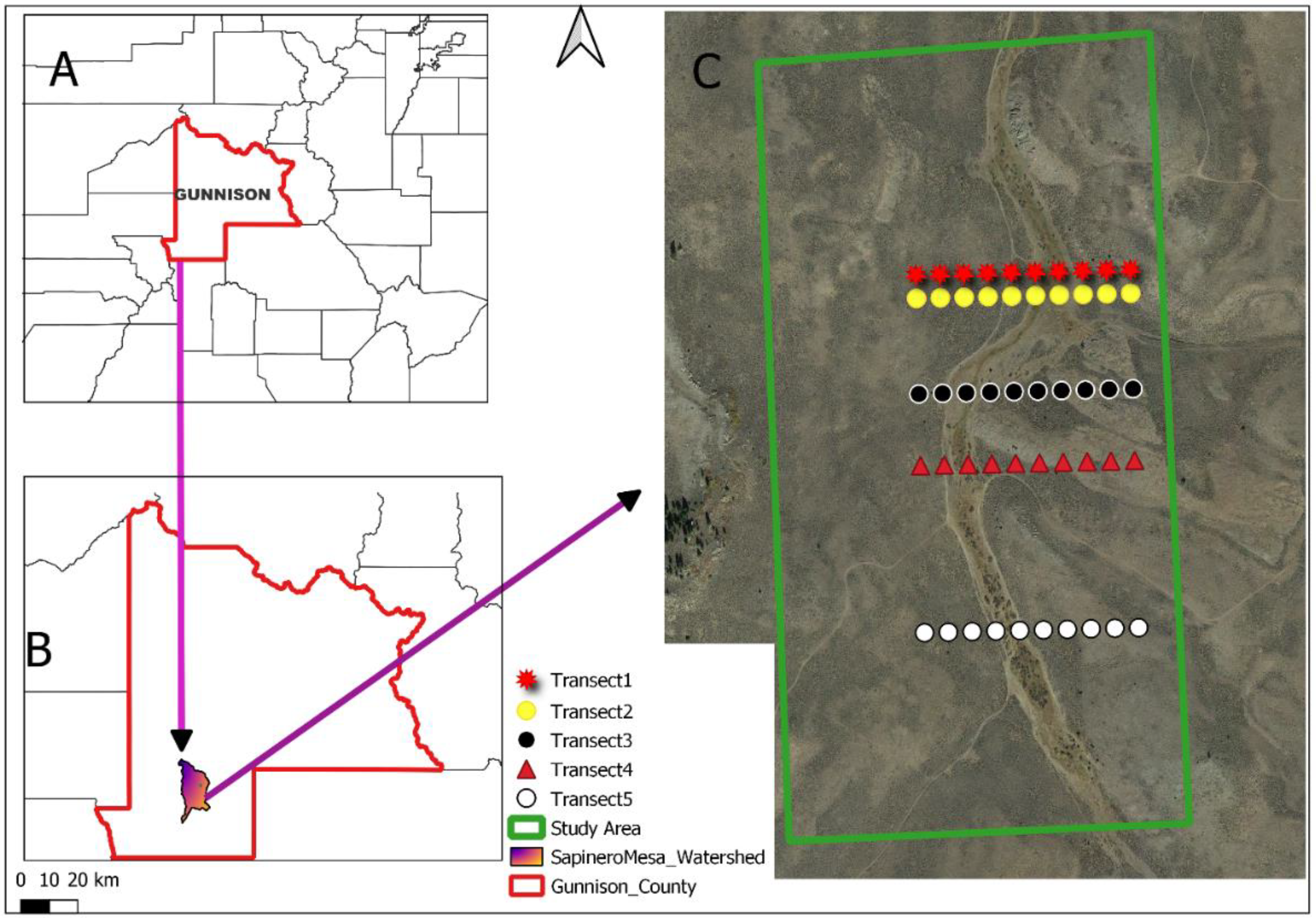
Figure 2.
Backscattering Coefficient Estimation Chart.
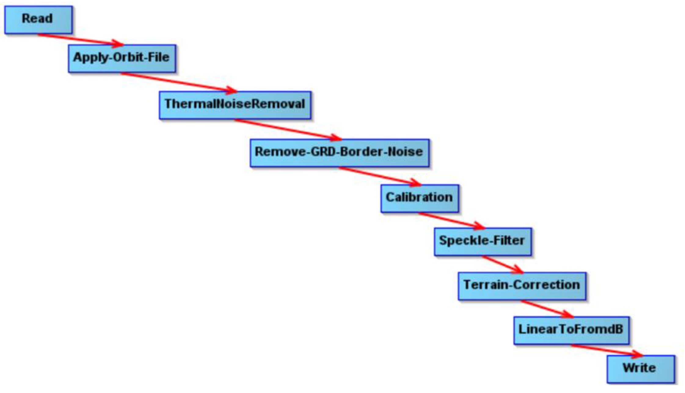
Figure 3.
The predicted versus observed plots of the best satellite/ground-data models across all depths. NSDSI2 at the depth of 0 – 5 cm; NSDSI2 at the depth of 0 – 10 cm; and NDVI at the depth of 0 – 20 cm. The red line on all plots indicates the line of best fit, and the blue line represents a 1:1 relationship.
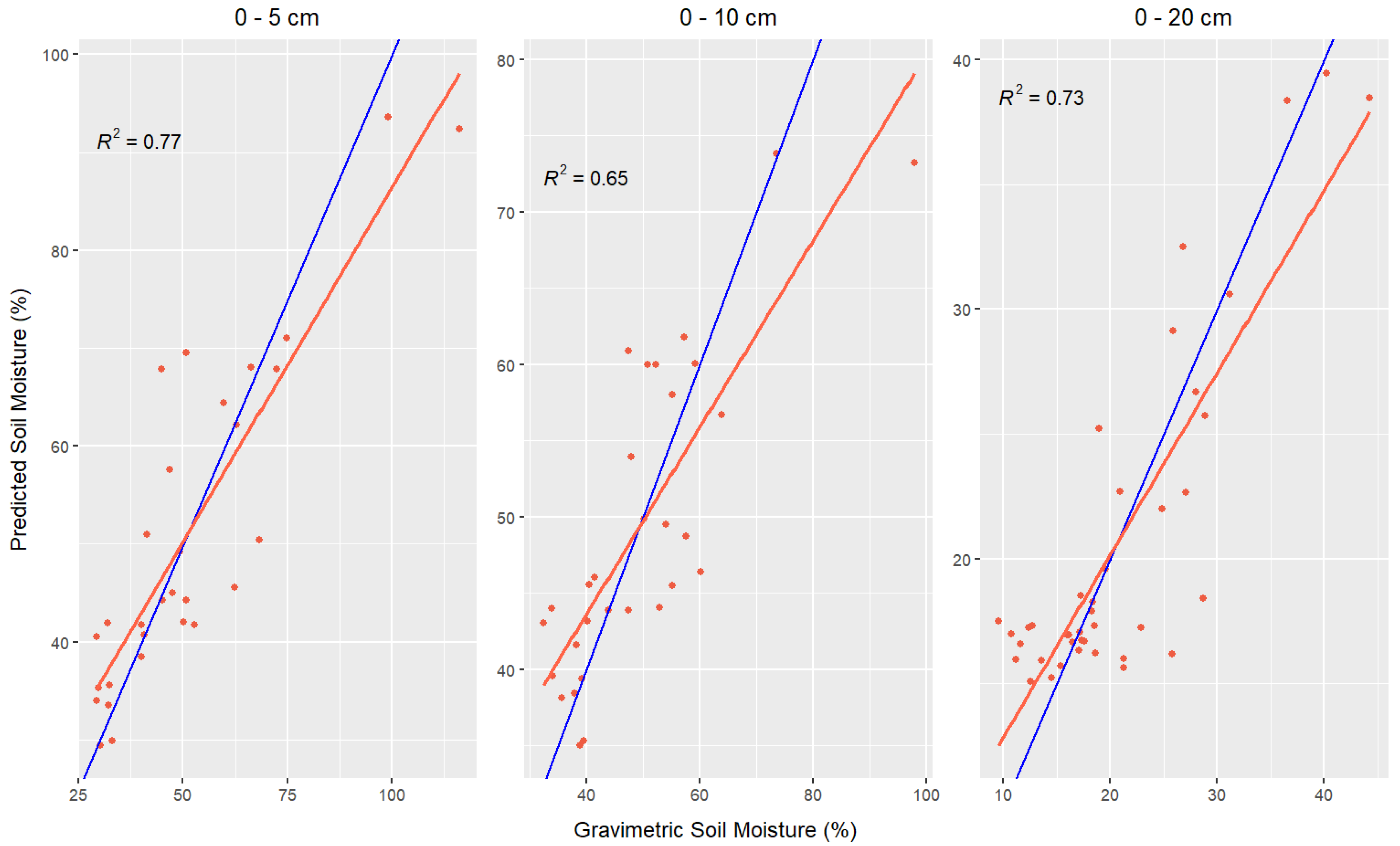
Figure 5.
The predicted versus observed plots of the best UAS/ground data models across all depths. NDRE at the depth of 0 – 5 cm; and NDVI at the depth of 0 – 10cm. As in Figure 4, the red line on all plots indicates the line of best fit, and the blue represents a 1:1 relationship.
Figure 5.
The predicted versus observed plots of the best UAS/ground data models across all depths. NDRE at the depth of 0 – 5 cm; and NDVI at the depth of 0 – 10cm. As in Figure 4, the red line on all plots indicates the line of best fit, and the blue represents a 1:1 relationship.
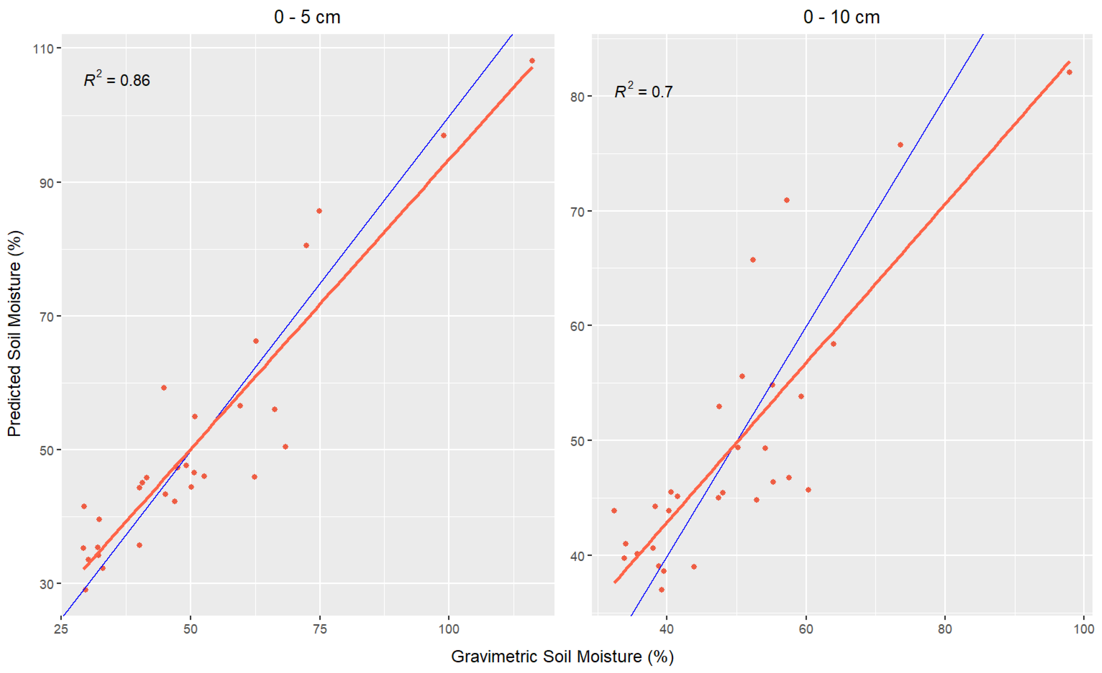

Table 1.
Specifications of the remote sensing images used.
| Acquisition Dates | Imagery/Data | Specifications | Spatial resolution | |
| Aug 1/Sept 9 | Landsat-9 | Path/Row | 33/34 | 30 m (OLI-2) |
| July 28/Sept 9 | Sentinel 1A | Imaging Frequency Acquisition-orbit Data Product |
5.4GHz Descending Level-1 GRD |
10 m |
| Sept 9 | E2 UAS | L-Band | 1-2 GHz | 0.55 * 0.41 m 0.04 * 0.03 m |
Table 2.
Specifications of variables analyzed from remotely sensed images.
| Variables | Remote sensed source |
| NSDSI2 | Landsat-9 |
| NDVI | Landsat-9; E2 UAS |
| dB | Sentinel-1A |
| NDRE | E2 UAS |
| ENDVI | E2 UAS |
| GRVI | E2 UAS |
| GLI | E2 UAS |
Note: NSDSI2 – Normalized Shortwave-Infrared Soil Moisture Index; NDVI – Normalized Difference Vegetation Index; dB – Backscattering Coefficient; NDRE – Normalized Difference Red Edge Index, ENDVI – Enhanced Difference Vegetation Index, GRVI – Green-Red Vegetation Index, GLI – Green Leaf Index.
Table 3.
Sample size for GSM and VSM measured from ground-based sampling at Sapinero Mesa, Colorado.
Table 3.
Sample size for GSM and VSM measured from ground-based sampling at Sapinero Mesa, Colorado.
| Date | Depth (cm) | Sample size | |
| GSM | VSM | ||
| August 1&2, 2022 | 0 – 7.6 | - | 50 |
| 0 – 10 | 50 | - | |
| 0 – 20 | 48 | 49 | |
| September 9, 2022 | 0 – 5 | 30 | - |
| 0 – 7.6 | - | 30 | |
| 0 – 10 | 30 | - | |
Table 4.
Distribution of soil moisture across sampling points and sampling times. Soil moisture (SM), percent (%), standard error (SE).
Table 4.
Distribution of soil moisture across sampling points and sampling times. Soil moisture (SM), percent (%), standard error (SE).
| Month | Depth (cm) | SM | Range (%) | Mean | SE |
| August | 0 – 20 | GSM | 9.56 – 44.26 | 20.64 | 1.26 |
| 0 – 10 | GSM | 10.56 – 89.81 | 34.07 | 2.98 | |
| 0 – 20 | VSM | 11.80 – 40.60 | 24.91 | 1.18 | |
| 0 – 7.6 | VSM | 10.20 – 58.00 | 26.35 | 1.26 | |
| September | 0 – 10 | GSM | 32.42 – 97.90 | 49.33 | 2.49 |
| 0 – 5 | GSM | 29.94 – 116.08 | 51.01 | 3.74 | |
| 0 – 7.6 | VSM | 1.70 – 15.70 | 7.24 | 0.70 |
Table 5.
Best Fitted Models between Remote Sensing Indices and SM data (GSM) across all depths and sampling times.
Table 5.
Best Fitted Models between Remote Sensing Indices and SM data (GSM) across all depths and sampling times.
| RS Data | Month | Depth (cm) | Predictor Variables | R2 | RMSE | MAE | Models |
| Landsat 9 | August | 0 – 20 | NDVI | 0.73 | 4.09 | 3.32 | Y = 5.5 +0.73x |
| September | 0 – 10 | NSDSI2 | 0.65 | 7.91 | 5.98 | Y = 19 +0.61x | |
| 0 – 5 | NSDSI2 | 0.77 | 9.79 | 7.11 | Y = 14 +0.72x | ||
| E2 UAS | September | 0 – 10 | NDVI | 0.70 | 7.31 | 5.91 | Y = 15 +0.69x |
| 0 – 5 | NDRE | 0.86 | 7.41 | 5.86 | Y = 6.9 +0.86x |
Note: The highlighted rows show the best models across different depths based on the highest R2 values, lowest RMSEs, AND lowest MAEs.
Disclaimer/Publisher’s Note: The statements, opinions and data contained in all publications are solely those of the individual author(s) and contributor(s) and not of MDPI and/or the editor(s). MDPI and/or the editor(s) disclaim responsibility for any injury to people or property resulting from any ideas, methods, instructions or products referred to in the content. |
© 2024 by the authors. Licensee MDPI, Basel, Switzerland. This article is an open access article distributed under the terms and conditions of the Creative Commons Attribution (CC BY) license (http://creativecommons.org/licenses/by/4.0/).
Copyright: This open access article is published under a Creative Commons CC BY 4.0 license, which permit the free download, distribution, and reuse, provided that the author and preprint are cited in any reuse.


