Preprint
Article

A New Hyperspectral Change Detection (HCD-Net) Framework Based on Double Stream CNN and Attention Module

Altmetrics

Downloads

194

Views

165

Comments

0

A peer-reviewed article of this preprint also exists.

Submitted:

11 January 2024

Posted:

11 January 2024

You are already at the latest version

Alerts
Abstract
Human activities and natural events alter the earth’s surface and pose a constant threat to the environment. Thus, accurately monitoring and predicting these changes in a timely manner is crucial to provide solutions and mitigate the environmental consequences beforehand. This research introduces a novel framework, called HCD-Net, for change detection using bi-temporal hyperspectral images. The framework is based on double-stream deep feature extraction and an attention mechanism. The first stream focuses on deep feature extraction through 3D convolution layers and 3D Squeeze-and-Excitation (SE) blocks. The second stream focuses on deep feature extraction through 2D convolution and 2D SE blocks. The extracted deep features are then concatenated and fed to dense layers for decision-making. The efficiency of HCD-Net is compared to the state-of-the-art change detection methods. Additionally, the bi-temporal Airborne Visible InfraRed Imaging Spectrometer (AVIRIS) hyperspectral dataset was used for further evaluation of the change detection results. The results show that HCD-Net has a higher accuracy and the lowest false alarm rate, where the overall classification accuracy is above 96%, and the kappa coefficient is over 0.9.
Keywords: 
Subject: Environmental and Earth Sciences  -   Remote Sensing

1. Introduction

The changes on the Earth stem from both natural hazards (e.g., floods and earthquakes) and human activities (e.g., urban development) [1]. Therefore, Change Detection (CD) algorithms are crucial tools for disaster and resource management. There are several methods of landscape CD, one of the most important of which is Remote Sensing (RS) [2,3]. RS data measure the changes between objects in a specific region over time [4]. It is a valuable source of data with different advantages, including frequent coverage, the ability to monitor large-scale areas, and low cost [5]. RS data can be used for various CD applications, including fire monitoring [6,7], climate change [8,9,10,11,12,13], and flood mapping [14,15,16,17].
One type of RS imagery that provides better spectral resolution is Hyperspectral RS imagery (HIS) [18,19,20,21]. HIS improves the process of CD for similar targets due to its high number of spectral bands [22,23], compared to multispectral imagery. The hyperspectral sensors can be divided into two categories: (1) airborne (e.g., Airborne Visible/Infrared Imaging Spectrometer (AVIRIS)); and (2) space-borne (e.g., Recursore IperSpettrale della Missione Applicativa (PRISMA), Enmap). In the near future, new space-borne sensors will be deployed (HyspIRI, SHALOM, and HypXIM) [24]. Multiple studies have so far used HIS for CD [24,25,26,27]. The specific nature of HIS has made extracting multi-temporal imagery a significant challenge [28]. As a result, this remains a dynamic and challenging area of study. Atmosphere status, noise levels, and data overload are among the most challenging factors affecting the results of HCD [24]. Numerous methodologies have so far been proposed for HCD. For example, Ertürk et al. [29] suggested a CD technique by applying sparse spectral unmixing to bi-temporal hyperspectral images. First, this method predicts the changed areas using the spectral unmixing method, then creates a binary change map by thresholding the abundance maps. Ertürk [30] also designed an HCD framework based on a fuzzy fusion strategy; similarity measures indices, the spectral angle mapper (SAM) algorithm, and change vector analysis to predict changed areas. The fuzzy inference fusion strategy was used to fuse the magnitude and angle measurements obtained by the change vector analysis (CVA) and SAM algorithms, respectively. Additionally, López-Fandiño et al. [26] proposed a two-step HCD framework for performing binary and multi-CD. They first generated a binary change map based on segmentation and thresholding and using the SAM algorithm. Then, the image differencing algorithm was used to combine multi-temporal images. The Stacked Auto-encoders algorithm was then employed to reduce the dimensionality of HIS. Finally, the binary change map and the reduced HIS were used to produce the multi-class change map. In recent work, Ghasemian and Shah-Hosseini [31] also designed an HCD framework for multiple and binary CD based on several steps: (1) stacking the bi-temporal dataset and generating sample data based on the peak density clustering algorithm, (2) implementing target detection methods based on the produced sample data, (3) generating a binary change map based on the Otsu thresholding, (4) utilizing the sparse coding algorithm and the support vector domain description (SVDD) for generating multiple maps. Saha et al. Furthermore, [32] proposed an HCD framework based on an untrained deep model for HCD. This method extracts deep features for the first and second times of hyperspectral images using the untrained model and measures the similarity of the deep features through the Euclidean norm. The Otus algorithm is used to threshold the predicted deep features, resulting in a binary change map. Tong et al. [33] also proposed a framework for HCD by analyzing and transfer learning of uncertain areas. This method is applied in four main steps: (1) generating a binary change map according to the uncertain area analysis using K-Means clustering, CVA, and rule-based methods, (2) classifying the source image based on an active learning framework, (3) second-time image classification based on improved transfer learning and a support vector machine (SVM) classifier, and (4) utilizing post-classification analysis for multiple change map detection. Moreover, Seydi and Hasanlou [34] designed an HCD method based on a 3D convolutional neural network (3D-CNN) and an image differencing algorithm. This framework utilized the image differencing procedure to predict change and no-change areas and then employed the 3D-CNN to classify the change areas to generate a binary change map. Finally, Borsoi et al.[35] proposed a fast spectral unmixing method for HCD based on the high temporal correlation between the abundances. This method detects abrupt changes by considering the residuals of end-member selection.
Although the current HCD methods have shown promising results, they usually have several limitations, including the following items:
(1)
They require a threshold, and selecting a suitable threshold can be challenging.
(2)
They primarily focus on spectral data while ignoring the potential of spatial features in improving HCD results, which has been proven by multiple studies.
(3)
Most HCD methods are complex to implement and require high-complexity computation.
(4)
Noise and atmospheric conditions can negatively affect the automatic generation of pseudo-sample data through simple predictors and thresholding methods.
(5)
Most HCD methods require additional pre-processing steps, such as highlighting changes (recognizing changes from no-changes) or dimensional reduction. The dependence of HCD results on the chosen method for conducting these pre-processing steps makes it difficult to obtain robust results in different study areas.
Given these limitations, a novel method has been proposed in this study to minimize the challenges and to improve HCD results. This study introduces a new framework for HCD based on double-stream CNNs called the HCD-Net. The HCD-Net uses multiscale 3D/2D convolution layers and 3D/2D attention blocks. The advantages of the HCD-Net are: (1) using the multiscale multi-dimensional kernel, (2) utilizing 3D/2D attention blocks, (3) high efficiency, and providing robust results in HCD. The key contributions of this study are:
(1)
Proposing a double-stream deep feature extraction method for HCD using 3D/2D convolution layers.
(2)
Implementing the HCD-Net in an End-to-End manner without additional processing.
(3)
Taking advantage of the 3D/2D attention mechanism for informative deep feature extraction.
(4)
Evaluating the efficiency of HCD methods in different areas using both space-borne and airborne HIS.

2. Methodology

The HCD-Net is designed in three main steps: (1) Pre-processing, (2) tuning parameters and model training, and (3) CNN-based binary classification and accuracy assessment. The details of the HCD-Net are presented in Figure 1 and are further discussed in the following subsections.

2.1. Pre-Processing

The RS datasets require pre-processing steps before they can be utilized for CD. These steps can be divided into spectral and spatial corrections. The pre-processing includes spectral correction followed by a subsequent spatial correction. Spectral rectification of the hyperspectral level-1 raw (L1R) Hyperion data (space-borne sensor) involved eliminating bands with no-data values, de-striping, de-noising, smile, radiometric, and atmospheric corrections. During preprocessing, the geometric correction was also performed. After pre-processing, 154 spectral bands were used in this study for HCD. The pre-processing step for the airborne sensor (AVIRIS) has already been completed, and the pre-processed data is used in this article.

2.2. CNN-based HCD

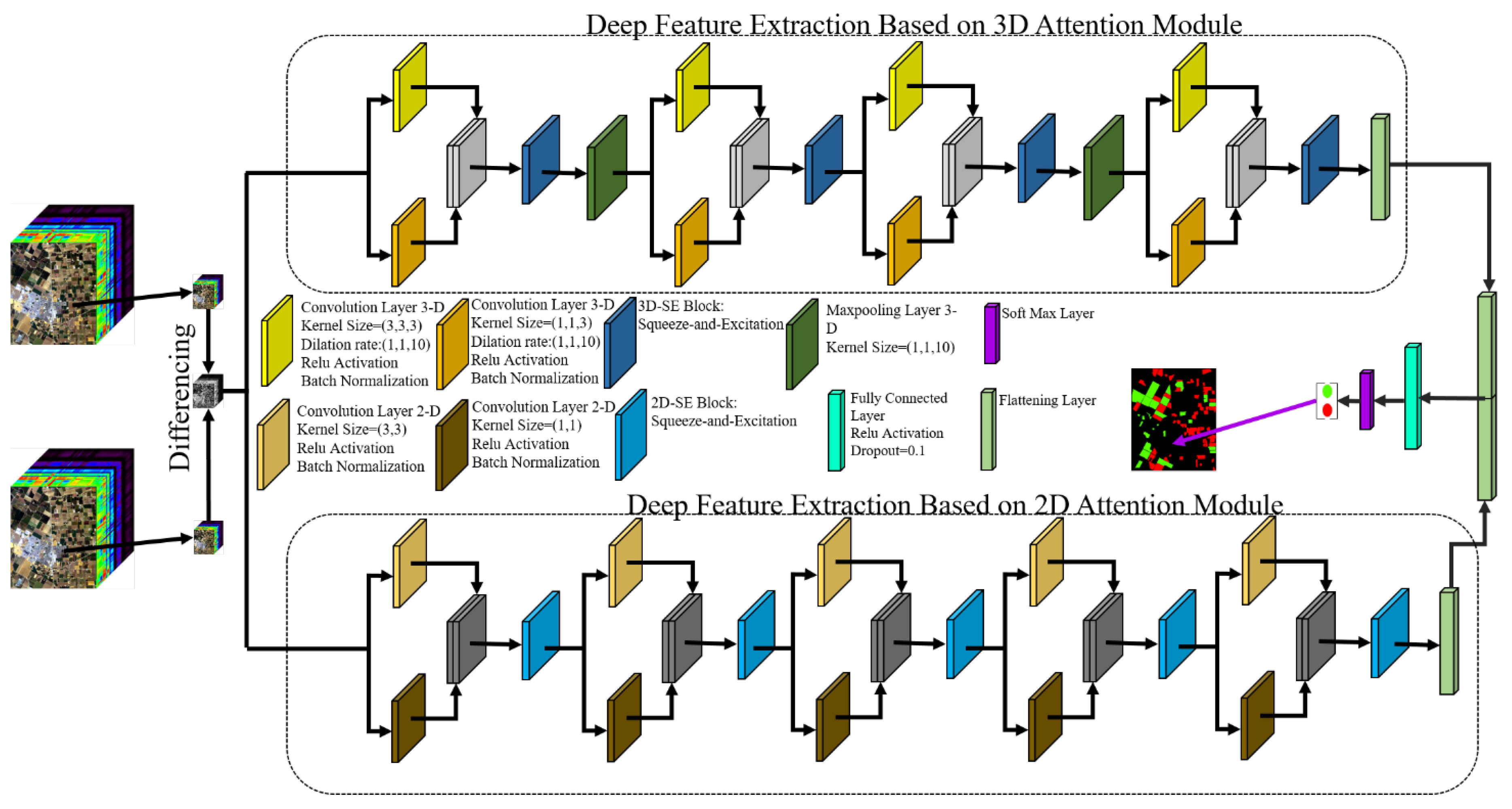
Deep Learning (DL) methods can automatically absorb informative proxies of input datasets with a high degree of abstraction [36]. Among all DL frameworks, including CNNs, deep belief networks (DBNs), generative adversarial networks (GANs), recurrent NN (RNN), and auto-encoder (AE), CNN is the most common method [37]. CNN is one of the most popular DL-based frameworks and has applications in various fields. It uses stacked convolutional kernels to learn the spectral and texture information in the spatial domain [38]. It can classify inputs based on the interrelationships between the input data and target labels. The CNN network has two main components: a feature extractor and a softmax classifier, which is typically implemented as a multi-layer perceptron (MLP) and assigns the class label. The CNN network includes several operational layers, such as convolution layers, pooling layers, nonlinear activation functions, and normalization layers [20]. This research proposes a novel double-stream HCD framework using a CNN network. Figure 2 illustrates the architecture of the proposed dual-stream CNN framework for HCD. Firstly, the two input patch datasets are combined into a single patch dataset through image differencing to reduce computation time and processing. However, many DL-based frameworks stack the input patch data. The result of this differencing is fed into a double-stream channel to extract deep, high-level features. The first channel utilizes multi-scale 3D convolution blocks, pooling layers, and 3D-SE blocks. The second stream focuses on the extraction of 2D deep features using 2D convolution layers and 2D-SE blocks. It is deeper than the first stream and contains more multiscale coevolution blocks, but it does not utilize pooling layers. Initially, the input dataset is fed into a multiscale 2D convolution block, followed by the 2D-SE attention block to extract informative features. This channel comprises five multiscale convolution blocks and five 2D-SE blocks. The final layer is a flattening layer, which reshapes the deep features into a 1-D vector map. The deep features extracted by the two streams are concatenated by the concatenating layer and fed into the classification layers. The fully connected layer is employed in the classification part to create a connection between the CNN and MLP layers. After the fully connected layers, the soft-max layer is used to decide on the input feature data.
The HCD-Net has several differences compared to the HCD frameworks, including
(1)
Taking advantage of SE-bock in extracting informative deep features.
(2)
Utilizing the advantages of spectral information in the hyperspectral dataset through 3D convolution layers.
(3)
Combining 3D and 2D convolutions to explore high-level spectral and spatial information.
(4)
Utilizing a multiscale convolution block to increase the robustness of the network against different object sizes.
(5)
Employing a differencing algorithm to reduce computational and time costs instead of concatenating deep features in the first layers.
The multidimensional kernel convolution used in this study encompasses 3-D, 2-D, and 1-D kernel convolution. The distinction between these kernel convolutions is illustrated in Figure 3.

2.3. Squeeze and Excitation (SE) Blocks

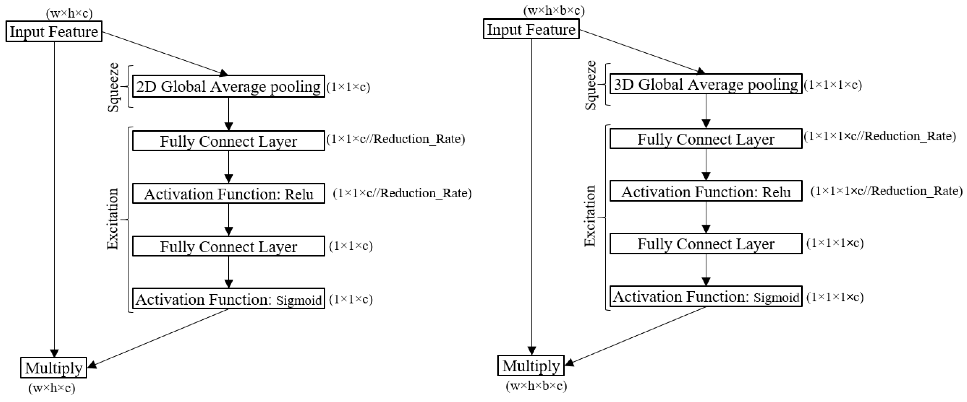
The proposed SE block adjusts channel-wise feature responses adaptively to explicitly model the interconnections between channels, thus improving channel interdependencies with minimal computational cost. The block consists of three components: (1) Squeeze, (2) Excitation, and (3) Rescale. The Squeeze module uses global average pooling (GAP) to reduce the spatial dimensions of the input feature data to a singular value. The Excitation module then investigates the output of the Squeeze module, learning adaptive scaling weights for the feature through two MLP layers with Relu (neurons in the first layer) and Sigmoid (neurons in the second layer) activation functions, respectively. Finally, the Rescale component uses element-wise multiplication to return the features to their original size. In this research, 3D/2D SE blocks are used in the proposed architecture for HCD. Figure 3 illustrates the differences between 2D/3D SE blocks. The main difference between the two blocks is noted in the Squeeze module, where the 3D Squeeze module uses a 3D GAP, and the 2D Squeeze module uses a 2D GAP.

2.4. Convolution Layers

The convolution layers form the central core of CNN network frameworks and are capable of exploiting deep and high-level features. They can be categorized into three types based on their filter size: (1) 3D kernel convolution, (2) 2D kernel convolution, and (3) 1-D kernel convolution. The proposed architecture leverages the benefits of both 3D and 2D convolution layers to extract deep features. Additionally, this research incorporates multiscale convolution blocks to enhance the network’s resilience against variations in object size.
The strength of 3D convolution layers lies in consideration of both spatial and spectral features. In other words, the 3D convolution layers consider the relation between the central pixel with its neighborhood and the relation between spectral bands. The feature map (H) for the 3D-convolution layer at position (alpha, beta, gamma) on the y t h feature of the x t h layer is given by Eq. (1).
H ( x , y ) ( α , β , γ ) = F b ( x , y ) + τ = 1 m ( l 1 ) i = r r j = s s k = t t W ( x , y , τ ) ( r , s , t ) H ( x 1 , i ) ( α + r , β + s , γ + t )
where F is the activation function, b(x,y) is the bias parameter, m is the number of feature maps in the ( l 1 ) t h layer; 2r+1,2s+1, and 2t+1 are the width, height, and depth of kernel along a spectral dimension, respectively. In the 2D convolution layer, the feature map value at position ( α , β ) can be enumerated using the below equation:
H ( x , y ) ( α , β ) = F b ( x , y ) + τ = 1 m ( l 1 ) i = r r j = s s W ( x , y , τ ) ( r , s ) H ( x 1 , i ) ( α + r , β + s )
The activation function is a rectified linear unit (Relu) according to the following equation:
f ( x ) = max { 0 , x }
Furthermore, the Sigmoid activation function can be formulated by equation 4.
f ( x ) = e x 1 + e x

2.5. Model Parameters Optimization

The HCD-Net has parameters that are estimated using a back-propagation method to find the optimal values. The model parameters are iteratively tuned by an optimizer based on the loss value. To achieve this, the model is trained using the training sample data, with the initial parameters initialized by the He-Normal method. The network error is then calculated using a loss function on the validation dataset. The optimizer updates the network parameters based on the feedback from the loss value. The Adam optimization algorithm is utilized to tune the parameters of the model. Furthermore, the cost function used is binary cross-entropy, as follows:
H p ( q ) = 1 2 [ y 1 log ( p ( y 1 ) ) + y 2 log ( p ( y 2 ) ) + ( 1 y 1 ) log ( 1 p ( y 1 ) ) + ( 1 y 2 ) log ( 1 p ( y 2 ) ) ]
where y is a label (true value) and p(y) is the predicted probability observation.

2.6. Accuracy Assessment and Comparison with Other Methods

The primary purpose of this step is to evaluate the results obtained by comparing them with the reference dataset. To achieve this, several comparison indices, including Overall Accuracy (OA), Kappa Coefficient (KC), F1-Score, Recall, Precision, and Balance Accuracy (BA), were used for accuracy assessment. The results were also compared with three state-of-the-art methods: the 2D Siamese Network, the 3D Siamese Network, and General End-to-end Two-dimensional CNN Framework (GETNET) [40]. The 2D Siamese Network has two deep feature extraction channels, with the first channel analyzing the first-time hyperspectral dataset and the second channel focusing on the after-change hyperspectral dataset. Similarly, the 3D Siamese Network has a similar architecture but utilizes 3D convolution layers.

3. Case Study

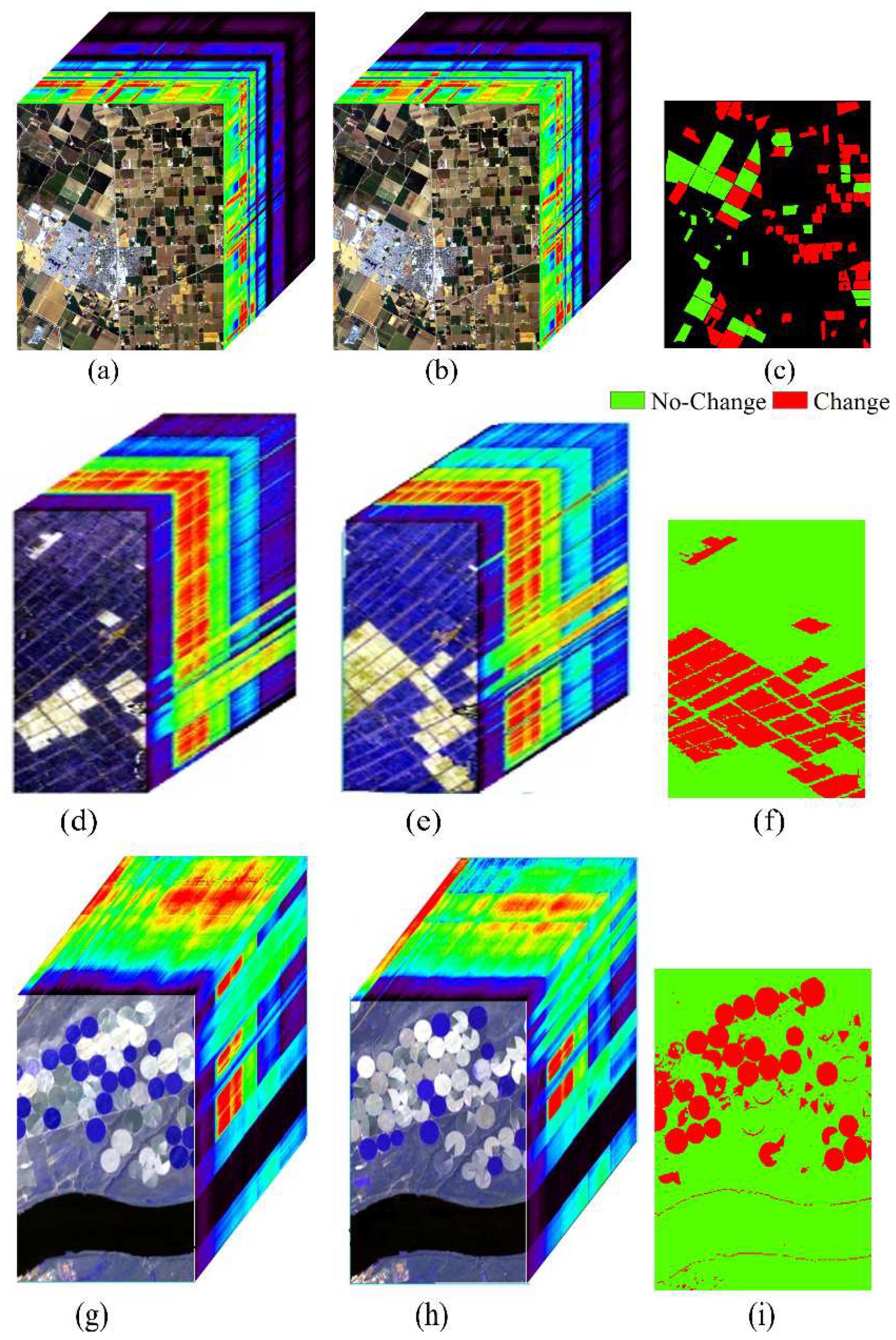
The HCD-Net is evaluated using two HISs for the purpose of evaluating various types of HCD methods. The quality of the ground truth data is a critical factor in these evaluations; hence the selection of these datasets is primarily due to their access to control datasets, which are widely utilized in various HCD studies such as, [39,40]. In these studies, the ground control datasets were created through visual inspection. The first dataset was acquired near Yuncheng Jiangsu province in China on May 3, 2006, and April 23, 2007. Soil, river, tree, building, roads, and agricultural fields are the main characteristics of this location. The second dataset was collected from irrigated agricultural fields in Hermiston, a city in Umatilla County, Oregon, USA, on May 1, 2004, and May 8, 2007. The datasets from China and the USA belong to the Hyperion sensor (Figure 4). The third dataset is the product of the AVIRIS sensor taken in 2013 and 2015 from the Bay Area surrounding the city of Patterson, California. The land cover includes soil, irrigation fields, rivers, human constructions, cultivated lands, and grassland. In all datasets, changes are affiliated with the land cover type and water body areas.
The details of the used dataset and the sample dataset for three case study areas are shown in Table 1 and are illustrated in Figure 4. For a fair comparison, 5% of the samples from the USA and China datasets and 1% of the samples from the Bay Area ground reference data were used for training the network. The sample data is divided into three parts: (1) training data (72%), (2) validation data (18%), and (3) test data (10%).

4. Experiment and Results

4.1. Results of HCD for the Bay Area Dataset

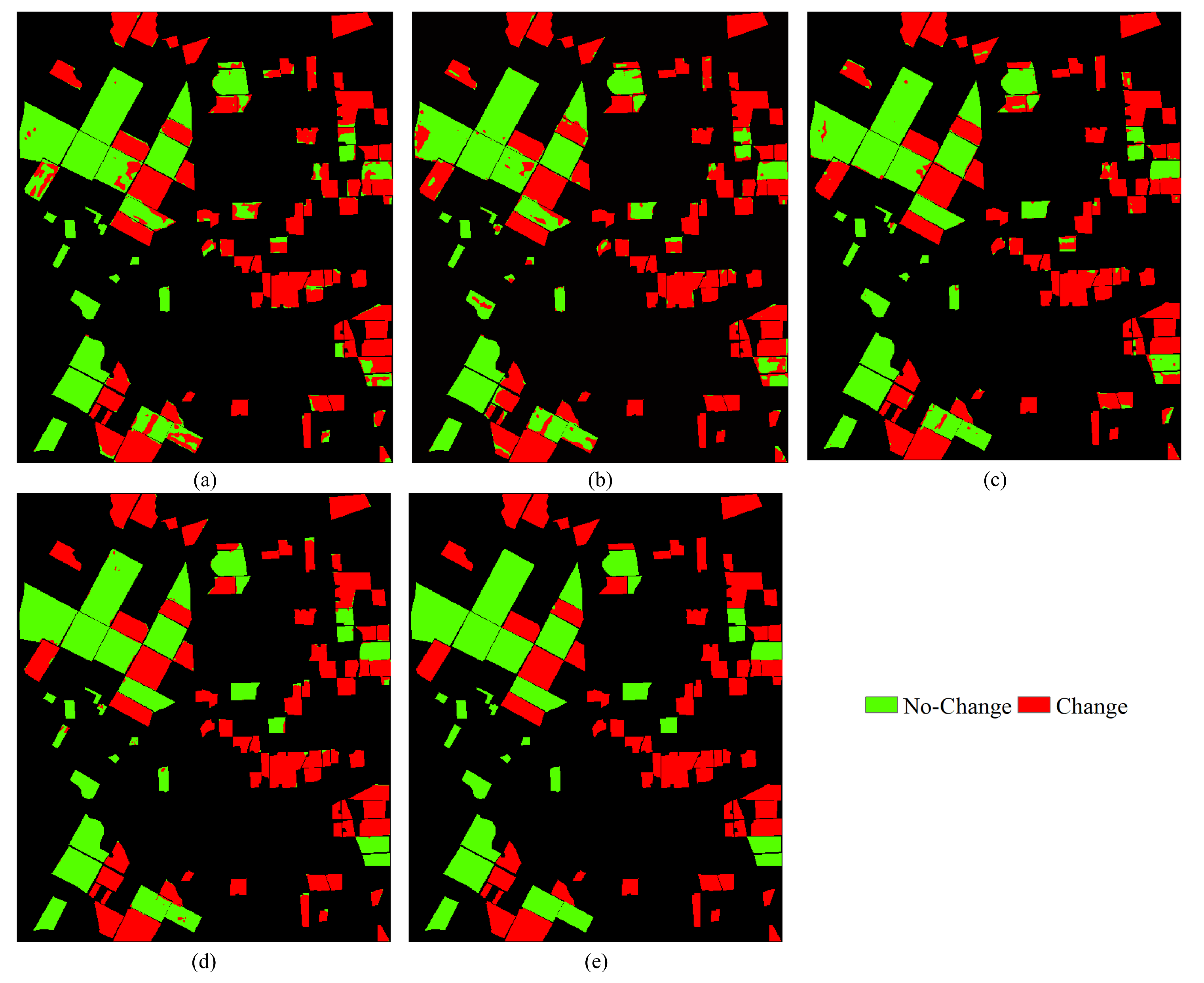
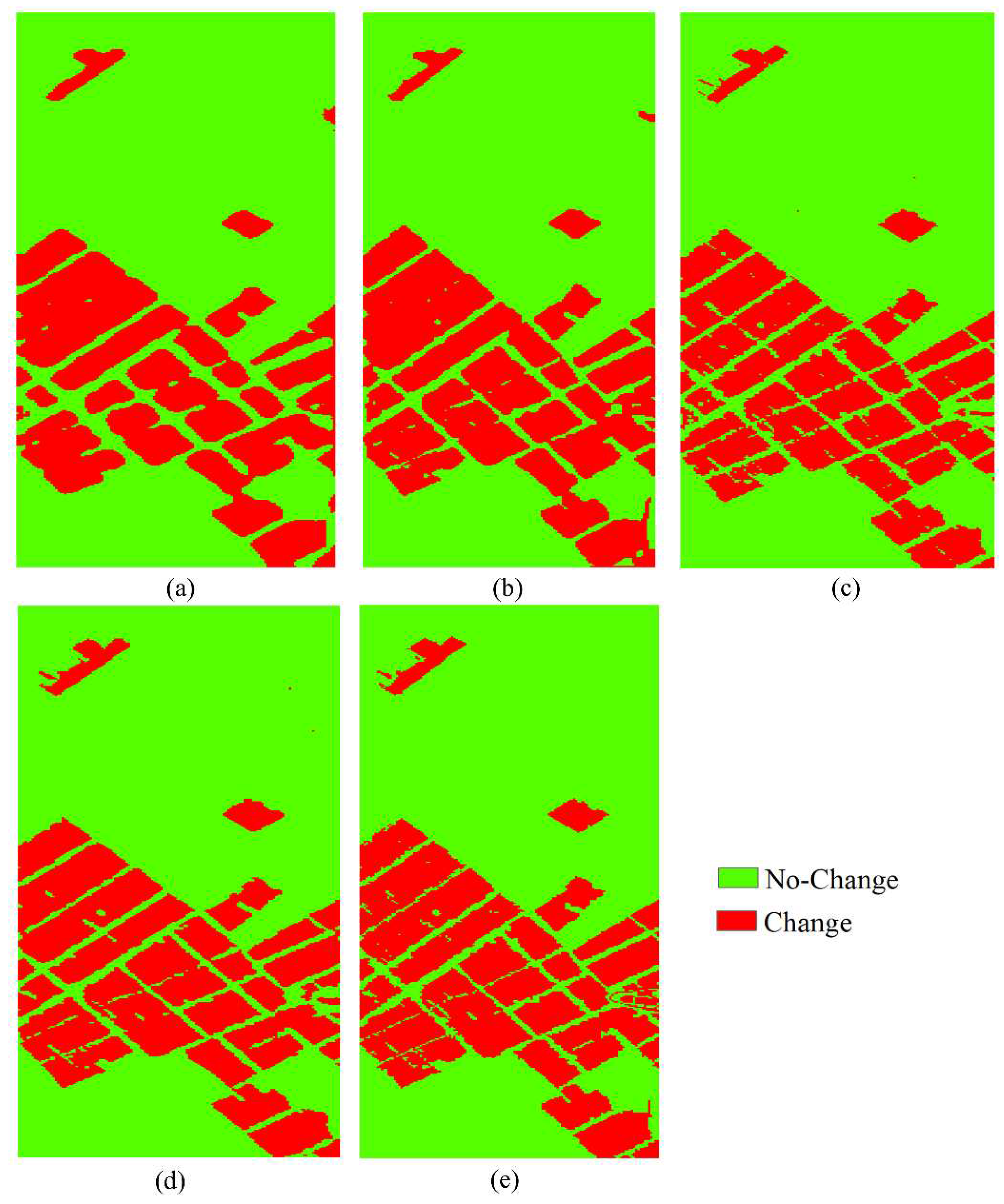
Figure 5 depicts the results of the HCD of the Bay Area dataset using four different CD methods. Most methods demonstrated high performance, although they vary in finer details. Several methods exhibit numerous false pixels in their results, while the HCD-Net precisely identified both the change and non-change pixels.
The numerical results of the HCD for the Bay Area dataset are presented in Table 2. Based on this table, most methods demonstrated an OA of over 91%. The HCD-Net improved the results of HCD by more than 2.42% in terms of OA, 2.94% in Precision, 1.51% in Recall, 2.33% in F1-Score, 2.48% in BA index, and 0.049 in KC index, compared to other methods.

4.2. Results of HCD for the China Dataset

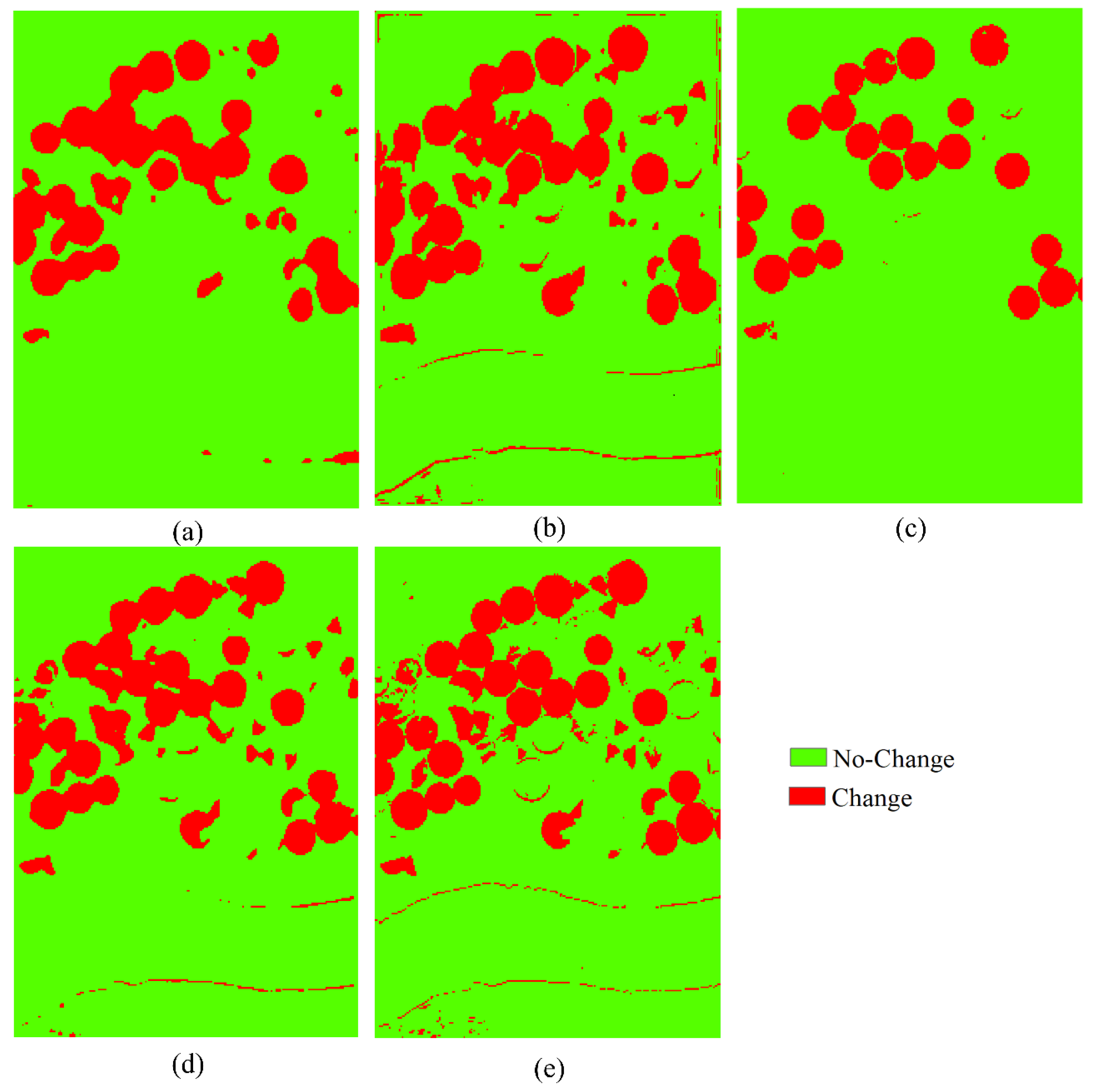
The results of the HCD methods applied to the China dataset are depicted in Figure 6. Most methods effectively identified both the change and no-change areas. Notably, HCD-Net better detected both classes (as indicated in Figure 6-d). On the other hand, there are numerous false pixels present in the results obtained from 2D-Siamese (Figure 6-a) and 3D-Siamese (Figure 6-b). Additionally, GETNET performed better in detecting no-change areas than change areas, but many change areas remain undetected (see Figure 6-c).
Table 3 presents the accuracies of the HCD methods for the China dataset. Based on numerical results, most methods provided OAs of more than 94% and KCs of more than 0.869. The higher performance of HCD-Net is clear when judged by the KC and BA indices, indicating that it has made significant improvement when compared to other methods. Although GETNET provided slightly better accuracy than HCD-Net based on Precision, it had lower performance according to other indices, especially KC, BA, Recall, and F1-Score.

4.3. Results of HCD for the USA Dataset

The results of the HCD methods applied to the China dataset are depicted in Figure 7. The numerical results of HCD are presented in Table 4 for the USA dataset. According to this Table, the majority of the methods had OAs of less than 93%, while the HCD-Net had an OA of more than 96%. The robustness of the HCD-Net is visible in most measurement indices. For instance, the improvement of the HCD-Net by the Recall and F1-Score is more than 5% compared to other models. Furthermore, the KC of the HCD-Net is 0.9, while other methods had values lower than 0.81. The GETNET provided a high accuracy by the Precision index, but has performed poorly in comparison with the HCD-Net using other indices.

5. Discussion

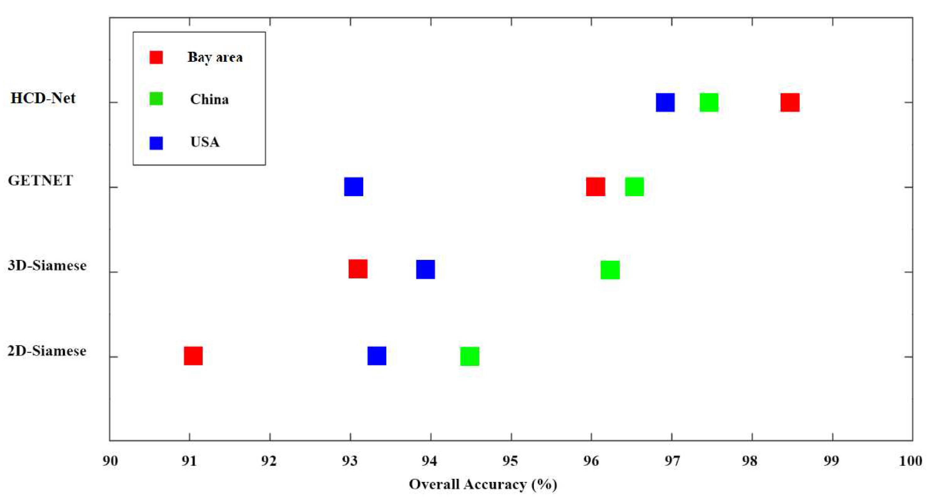
The results indicated that HIS has a high potential for CD purposes. For example, it was observed that the OAs for HCD of all methods were more than 90%. According to visual and statistical inspections, as shown in Figure 6 and Figure 7 and Table 2, Table 3 and Table 4, various methods provided different results for the study areas. However, the HCD-Net provided robust results in three case study areas. Compared to other methods, the variation in the values of KC is low in the HCD-Net. The mean KC value of the USA dataset is lower than the mean KCs of the other datasets. Thus, the complexity of the classes may affect the HCD results. Although this issue can be neglected in the HCD-Net results, other methods are highly dependent on the complexity of the dataset. Figure 8 illustrates the results of the OAs in the HCD for three study areas for all methods. The HCD-Net demonstrated promising results (more than 97%) for the three study areas, whereas the performance of other HCD methods was not satisfactory across all study areas.
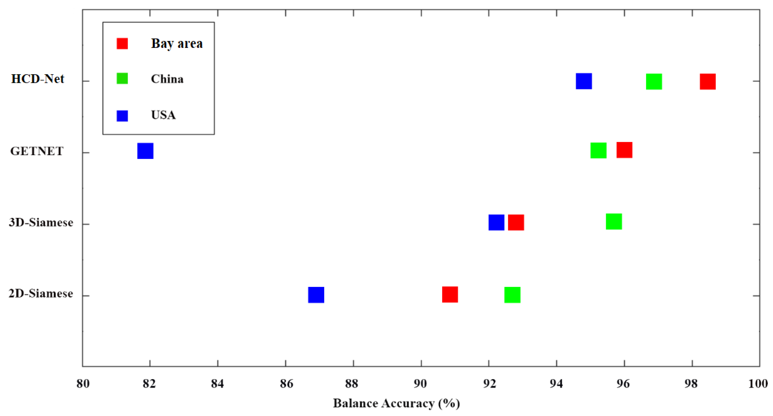
The performance of HCD methods by the BA index is presented in Figure 9. The BA index evaluates the performance of CD in both change and no-change classes. Due to the imbalanced datasets, most HCD algorithms focused on change or no-change areas while losing performance in both classes. Based on Figure 9, the HCD-Net had the highest performance, confirming the robustness of HCD-Net in HCD.
There is a trade-off between detecting change and no-change pixels in HCD. An accurate HCD method should provide robust and high performance in the detection of both classes. The HCD-Net could detect change and no-change pixels with a high level of accuracy, whereas other methods had lower performance in detecting both classes.
Many HCD methods ignore spatial features and focus mostly on spectral features. Moreover, although some methods incorporate spatial features, they do not use optimized features. Optimizing features can be challenging and time-consuming, which can cause a miss of HCD by traditional and other state-of-the-art methods. The HCD-Net automatically extracts deep features, involving both spatial and spectral features. As a result, when HCD is conducted using the HCD-Net, the results are highly accurate and reliable, particularly in large-scale areas where there is no ground truth to be examined. Additionally, the HCD-Net uses a multi-dimensional convolution layer, which improves the performance of HCD. The HCD-Net uses both 3D and 2D convolution, while many other HCD methods focus on 2D or 3D convolution layers. Furthermore, utilizing 3D/2D SE blocks helps extract informative deep features.
Several HCD methods for hyperspectral CD, such as GETNET, require additional processing, such as dimensional reduction and spectral unmixing. Due to the high dimensionality of the hyperspectral dataset, pre-processing the dataset is a big challenge. The HCD-Net does not require additional processing for HCD, while the GETNET algorithm uses spectral unmixing before CD.

6. Conclusions

A novel DL-based double-stream framework for HCD is proposed in this study. The proposed CD framework is based on multiscale 3D/2D convolution layers and attention mechanisms. Three bi-temporal HIS were used to evaluate the accuracy of HCD-Net. The HCD-Net was also compared to three other state-of-the-art methods. The results showed that the HCD-Net had several advantages compared to other state-of-the-art methods: (1) it provided higher accuracy (more than 96%), (2) it was robust and provided high accuracies at different study areas and using both airborne and spaceborne data, and (3) it did not require any additional processing before CD.

Author Contributions

Conceptualization, S.T.S., Z.N.; methodology, S.T.S., M.B., F.N.; validation, M.B., S.M.M.; writing—original draft preparation, S.T.S., M.B., F.N.; writing—review and editing, S.M.M., Z.N., M.A.; visualization, S.T.S., Z.N.; supervision, M.A.; project administration, M.A. All authors have read and agreed to the published version of the manuscript.

Funding

This research received no external funding.

Conflicts of Interest

The authors declare no conflict of interest.

Abbreviations

The following abbreviations are used in this manuscript:
AE Auto-Encoder
AVIRIS Airborne Visible InfraRed Imaging Spectrometer
BA Balance Accuracy
CD Change Detection
CNN Convolutional Neural Network
CVA Change Vector Analysis
DBN Deep Belief Network
DL Deep Learning
GAN Generative Adversarial Network
GAP Global Average Pooling
GETNET General End-to-end Two-dimensional CNN Framework
HCD-Net Hyperspectral Change Detection
HIS Hyperspectral RS Imagery
KC Kappa Coefficient
MPL Multi-Layer Perceptron
OA Overall Accuracy
PRISMA Recursore IperSpettrale della Missione Applicativa
RNN Recurrent Neural Network
RS Remote Sensing
SAM Spectral Angle Mapper
SVDD Support Vector Domain Description
SVM Support Vector Machine

References

  1. Zhan, T.; Gong, M.; Jiang, X.; Zhang, M. Unsupervised scale-driven change detection with deep spatial–spectral features for VHR images. IEEE Transactions on Geoscience and Remote Sensing 2020, 58, 5653–5665. [Google Scholar] [CrossRef]
  2. Renza, D.; Martinez, E.; Molina, I.; others. Unsupervised change detection in a particular vegetation land cover type using spectral angle mapper. Advances in Space Research 2017, 59, 2019–2031. [Google Scholar] [CrossRef]
  3. Marinelli, D.; Bovolo, F.; Bruzzone, L. A novel change detection method for multitemporal hyperspectral images based on binary hyperspectral change vectors. IEEE transactions on geoscience and remote sensing 2019, 57, 4913–4928. [Google Scholar] [CrossRef]
  4. Hussain, M.; Chen, D.; Cheng, A.; Wei, H.; Stanley, D. Change detection from remotely sensed images: From pixel-based to object-based approaches. ISPRS Journal of photogrammetry and remote sensing 2013, 80, 91–106. [Google Scholar] [CrossRef]
  5. Seydi, S.T.; Hasanlou, M. A new land-cover match-based change detection for hyperspectral imagery. European Journal of Remote Sensing 2017, 50, 517–533. [Google Scholar] [CrossRef]
  6. Semmens, K.A.; Ramage, J. Investigating correlations between snowmelt and forest fires in a high latitude snowmelt dominated drainage basin. Hydrological Processes 2012, 26, 2608–2617. [Google Scholar] [CrossRef]
  7. Jolly, W.M.; Freeborn, P.H.; Page, W.G.; Butler, B.W. Severe fire danger index: A forecastable metric to inform firefighter and community wildfire risk management. Fire 2019, 2, 47. [Google Scholar] [CrossRef]
  8. Yang, J.; Gong, P.; Fu, R.; Zhang, M.; Chen, J.; Liang, S.; Xu, B.; Shi, J.; Dickinson, R. The role of satellite remote sensing in climate change studies. Nature climate change 2013, 3, 875–883. [Google Scholar] [CrossRef]
  9. Boueshagh, M.; Hasanlou, M. Estimating water level in the Urmia Lake using satellite data: a machine learning approach. The International Archives of Photogrammetry, Remote Sensing and Spatial Information Sciences 2019, 42, 219–226. [Google Scholar] [CrossRef]
  10. Jalali, J.; Ahmadi, A.; Abbaspour, K. Runoff responses to human activities and climate change in an arid watershed of central Iran. Hydrological Sciences Journal 2021, 66, 2280–2297. [Google Scholar] [CrossRef]
  11. Ahmadi, A.; Jalali, J.; Mohammadpour, A. Future runoff assessment under climate change and land-cover alteration scenarios: a case study of the Zayandeh-Roud dam upstream watershed. Hydrology Research 2022, 53, 1372–1392. [Google Scholar] [CrossRef]
  12. Shafique, A.; Seydi, S.T.; Alipour-Fard, T.; Cao, G.; Yang, D. SSViT-HCD: A Spatial Spectral Convolutional Vision Transformer for Hyperspectral Change Detection. IEEE Journal of Selected Topics in Applied Earth Observations and Remote Sensing 2023. [Google Scholar] [CrossRef]
  13. Tavakol Sadrabadi, M.; Innocente, M.S. Vegetation Cover Type Classification Using Cartographic Data for Prediction of Wildfire Behaviour. Fire 2023, 6, 76. [Google Scholar] [CrossRef]
  14. Brivio, P.; Colombo, R.; Maggi, M.; Tomasoni, R. Integration of remote sensing data and GIS for accurate mapping of flooded areas. International Journal of Remote Sensing 2002, 23, 429–441. [Google Scholar] [CrossRef]
  15. Munawar, H.S.; Hammad, A.W.; Waller, S.T. Remote sensing methods for flood prediction: A review. Sensors 2022, 22, 960. [Google Scholar] [CrossRef] [PubMed]
  16. Maymandi, N.; Hummel, M.A.; Zhang, Y. Compound coastal, fluvial, and pluvial flooding during historical hurricane events in the Sabine-Neches Estuary, Texas. Water Resources Research 2022, e2022WR033144. [Google Scholar] [CrossRef]
  17. Naseri, K.; Hummel, M.A. A Bayesian copula-based nonstationary framework for compound flood risk assessment along US coastlines. Journal of Hydrology 2022, 610, 128005. [Google Scholar] [CrossRef]
  18. Hasanlou, M.; Seydi, S.T. Hyperspectral change detection: An experimental comparative study. International journal of remote sensing 2018, 39, 7029–7083. [Google Scholar] [CrossRef]
  19. Dong, W.; Xiao, S.; Liang, J.; Qu, J. Fusion of hyperspectral and panchromatic images using structure tensor and matting model. Neurocomputing 2020, 399, 237–246. [Google Scholar] [CrossRef]
  20. Fang, B.; Li, Y.; Zhang, H.; Chan, J.C.W. Collaborative learning of lightweight convolutional neural network and deep clustering for hyperspectral image semi-supervised classification with limited training samples. ISPRS Journal of Photogrammetry and Remote Sensing 2020, 161, 164–178. [Google Scholar] [CrossRef]
  21. Fathollahi, F.; Zhang, Y. Adaptive band selection for pan-sharpening of hyperspectral images. International Journal of Remote Sensing 2020, 41, 3924–3947. [Google Scholar] [CrossRef]
  22. Imani, M.; Ghassemian, H. An overview on spectral and spatial information fusion for hyperspectral image classification: Current trends and challenges. Information fusion 2020, 59, 59–83. [Google Scholar] [CrossRef]
  23. Takahashi Miyoshi, G.; Imai, N.N.; Garcia Tommaselli, A.M.; Antunes de Moraes, M.V.; Honkavaara, E. Evaluation of hyperspectral multitemporal information to improve tree species identification in the highly diverse atlantic forest. Remote Sensing 2020, 12, 244. [Google Scholar] [CrossRef]
  24. Seydi, S.T.; Hasanlou, M. A new structure for binary and multiple hyperspectral change detection based on spectral unmixing and convolutional neural network. Measurement 2021, 186, 110137. [Google Scholar] [CrossRef]
  25. Hong, D.; Wu, X.; Ghamisi, P.; Chanussot, J.; Yokoya, N.; Zhu, X.X. Invariant attribute profiles: A spatial-frequency joint feature extractor for hyperspectral image classification. IEEE Transactions on Geoscience and Remote Sensing 2020, 58, 3791–3808. [Google Scholar] [CrossRef]
  26. López-Fandiño, J.B.; Heras, D.; Argüello, F.; Dalla Mura, M. GPU framework for change detection in multitemporal hyperspectral images. International Journal of Parallel Programming 2019, 47, 272–292. [Google Scholar] [CrossRef]
  27. Ou, X.; Liu, L.; Tan, S.; Zhang, G.; Li, W.; Tu, B. A Hyperspectral Image Change Detection Framework With Self-Supervised Contrastive Learning Pretrained Model. IEEE Journal of Selected Topics in Applied Earth Observations and Remote Sensing 2022, 15, 7724–7740. [Google Scholar] [CrossRef]
  28. Bruzzone, L.; Liu, S.; Bovolo, F.; Du, P. Change detection in multitemporal hyperspectral images. Multitemporal Remote Sensing: Methods and Applications 2016, 63–88. [Google Scholar]
  29. Ertürk, A.; Iordache, M.D.; Plaza, A. Sparse unmixing-based change detection for multitemporal hyperspectral images. IEEE Journal of Selected Topics in Applied Earth Observations and Remote Sensing 2015, 9, 708–719. [Google Scholar] [CrossRef]
  30. Ertürk, S. Fuzzy fusion of change vector analysis and spectral angle mapper for hyperspectral change detection. IGARSS 2018-2018 IEEE International Geoscience and Remote Sensing Symposium. IEEE, 2018, pp. 5045–5048.
  31. Ghasemian, N.; Shah-Hosseini, R. Hyperspectral multiple-change detection framework based on sparse representation and support vector data description algorithms. Journal of Applied Remote Sensing 2020, 14, 014523–014523. [Google Scholar] [CrossRef]
  32. Saha, S.; Kondmann, L.; Zhu, X.X. Deep no learning approach for unsupervised change detection in hyperspectral images. ISPRS Annals of the Photogrammetry, Remote Sensing and Spatial Information Sciences 2021, 3, 311–316. [Google Scholar] [CrossRef]
  33. Tong, X.; Pan, H.; Liu, S.; Li, B.; Luo, X.; Xie, H.; Xu, X. A novel approach for hyperspectral change detection based on uncertain area analysis and improved transfer learning. IEEE Journal of Selected Topics in Applied Earth Observations and Remote Sensing 2020, 13, 2056–2069. [Google Scholar] [CrossRef]
  34. Seydi, S.; Hasanlou, M. Binary hyperspectral change detection based on 3D convolution deep learning. The International Archives of Photogrammetry, Remote Sensing and Spatial Information Sciences 2020, 43, 1629–1633. [Google Scholar] [CrossRef]
  35. Borsoi, R.A.; Imbiriba, T.; Bermudez, J.C.M.; Richard, C. Fast unmixing and change detection in multitemporal hyperspectral data. IEEE Transactions on Computational Imaging 2021, 7, 975–988. [Google Scholar] [CrossRef]
  36. Alom, M.Z.; Taha, T.M.; Yakopcic, C.; Westberg, S.; Sidike, P.; Nasrin, M.S.; Hasan, M.; Van Essen, B.C.; Awwal, A.A.; Asari, V.K. A state-of-the-art survey on deep learning theory and architectures. electronics 2019, 8, 292. [Google Scholar] [CrossRef]
  37. Ball, J.E.; Anderson, D.T.; Chan, C.S. Comprehensive survey of deep learning in remote sensing: theories, tools, and challenges for the community. Journal of applied remote sensing 2017, 11, 042609–042609. [Google Scholar] [CrossRef]
  38. Wang, L.; Zhang, J.; Liu, P.; Choo, K.K.R.; Huang, F. Spectral–spatial multi-feature-based deep learning for hyperspectral remote sensing image classification. Soft Computing 2017, 21, 213–221. [Google Scholar] [CrossRef]
  39. Jafarzadeh, H.; Hasanlou, M. An unsupervised binary and multiple change detection approach for hyperspectral imagery based on spectral unmixing. IEEE Journal of Selected Topics in Applied Earth Observations and Remote Sensing 2019, 12, 4888–4906. [Google Scholar] [CrossRef]
  40. Liu, S. Advanced techniques for automatic change detection in multitemporal hyperspectral images. PhD thesis, University of Trento, 2015.
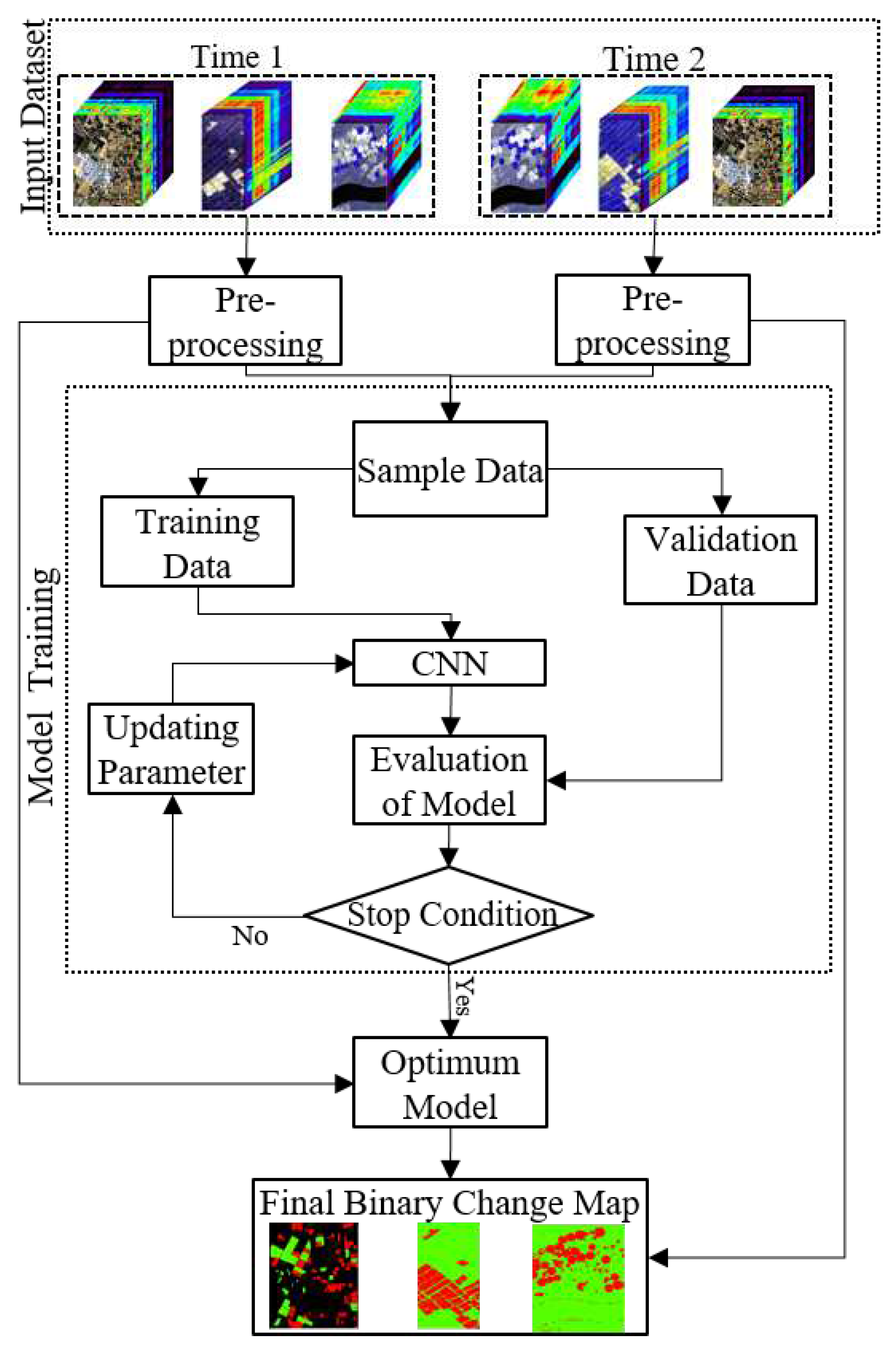
Figure 1. Flowchart of the proposed HCD-Net.
Preprints 96084 g001
Figure 2. The architecture of the proposed CNN framework for HCD.
Preprints 96084 g002
Figure 3. The main difference between 2D/3D Squeeze and Excitation (SE) blocks.
Preprints 96084 g003
Figure 4. (a) and (b) show composite images of the original HIS collected from the China dataset in 2006 and 2007, respectively, and (c) presents a ground truth image in binary format for these datasets. (d) and (e) show false-color composites of the original hyperspectral images from the USA dataset, acquired in 2004 and 2007, respectively, and (f) is the ground control data in binary format. (g) and (h) display hyperspectral images captured from the Bay Area dataset in 2013 and 2015, respectively, and (i) presents the ground truth data.
Preprints 96084 g004
Figure 5. The output of the binary HCD for the Bay Area dataset. (a) 2D-Siamese, (b) 3D-Siamese, (c) GETNET, (d) HCD-Net, and (e) Binary Ground Control.
Preprints 96084 g005
Figure 6. The result of the binary HCD for the China dataset. (a) 2D-Siamese, (b) 3D-Siamese, (c) GETNET, (d) HCD-Net, and (e) Binary Ground Truth.
Preprints 96084 g006
Figure 7. The result of the binary HCD for the USA dataset. (a) 2D-Siamese, (b) 3D-Siamese, (c) GETNET, (d) HCD-Net, and (e) Binary Ground Truth.
Preprints 96084 g007
Figure 8. OAs of different methods for HCD.
Preprints 96084 g008
Figure 9. BAs of different methods for HCD.
Preprints 96084 g009
Table 1. Details of the sample dataset incorporated for HCD in three study areas.
Dataset Size Data No-Change Change
Bay Area 600×500 73,404 34,211 39,270
China 420×140 58,800 40,417 18,383
USA 307×241 74,987 59,688 14,299
Table 2. Accuracy assessment of the HCD methods for the Bay Area dataset.
Index 2D-Siamese 3D-Siamese GETNET HCD-Net
OA (%) 91.05 93.10 96.05 98.47
Precision (%) 90.57 91.19 95.64 98.58
Recall (%) 92.92 96.40 97.04 98.55
F1-Score (%) 91.73 93.73 96.33 98.56
BA (%) 90.91 92.86 95.98 98.46
KC 0.820 0.861 0.920 0.969
Table 3. Accuracy assessment of different HCD methods for the China dataset.
Index 2D-Siamese 3D-Siamese GETNET HCD-Net
OA (%) 94.49 96.25 96.53 97.46
Precision (%) 94.43 93.63 97.28 96.69
Recall (%) 87.53 94.44 91.46 95.15
F1-Score (%) 90.85 94.03 94.28 95.92
BA (%) 92.59 95.76 95.15 96.83
KC 0.869 0.913 0.892 0.941
Table 4. Accuracy assessment of different HCD methods for the USA dataset.
Index 2D-Siamese 3D-Siamese GETNET HCD-Net
OA (%) 93.33 93.92 93.03 96.92
Precision (%) 87.13 81.18 100 92.53
Recall (%) 76.69 89.27 63.93 91.46
F1-Score (%) 81.58 85.03 78.00 91.99
BA (%) 86.98 92.15 81.96 94.85
KC 0.775 0.812 0.740 0.900
Disclaimer/Publisher’s Note: The statements, opinions and data contained in all publications are solely those of the individual author(s) and contributor(s) and not of MDPI and/or the editor(s). MDPI and/or the editor(s) disclaim responsibility for any injury to people or property resulting from any ideas, methods, instructions or products referred to in the content.
Copyright: This open access article is published under a Creative Commons CC BY 4.0 license, which permit the free download, distribution, and reuse, provided that the author and preprint are cited in any reuse.
Prerpints.org logo

Preprints.org is a free preprint server supported by MDPI in Basel, Switzerland.

Subscribe

© 2024 MDPI (Basel, Switzerland) unless otherwise stated