Preprint
Article
Advancing Global Pose Refinement: A Linear, Parameter-Free Model for Closed Circuits via Quaternion Interpolation
Altmetrics
Downloads
171
Views
53
Comments
0
A peer-reviewed article of this preprint also exists.
This version is not peer-reviewed
Submitted:
10 January 2024
Posted:
11 January 2024
You are already at the latest version
Alerts
Abstract
Global pose refinement is a significant challenge within Simultaneous Localization and Mapping (SLAM) frameworks. For LIDAR-based SLAM systems, pose refinement is integral to correcting drift caused by the successive registration of 3D point clouds collected by the sensor. A divergence between the actual and calculated platform path characterizes this error. In response to this challenge, we propose a linear, parameter-free model, which uses a closed circuit for global trajectory corrections. Our model maps rotations to quaternions and uses Spherical Linear Interpolation (SLERP) for transitions between them. The intervals are established from the constraint set by the Least Squares (LS) method on rotation closure and are proportional to the circuit's size. Translations are globally adjusted in a distinct linear phase. Additionally, we suggest a coarse-to-fine pairwise registration method, integrating Fast Global Registration and Generalized ICP with multiscale sampling and filtering. The proposed approach is tested on three varied datasets of point clouds, including Mobile Laser Scanners and Terrestrial Laser Scanners. These diverse datasets affirm the model's effectiveness in 3D pose estimation with substantial pose differences and efficient pose optimization in larger circuits.
Keywords:
Subject: Computer Science and Mathematics - Computer Vision and Graphics
1. Introduction
Inhabiting a three-dimensional world inherently challenges our ability to fully map an object's surface without adjusting the object's position or the sensor's viewpoint during the process. This difficulty gives rise to the Simultaneous Localization and Mapping (SLAM) problem, which aims to pinpoint the sensor's location at each mapping instance while simultaneously generating a comprehensive global map of the observed scenes. The crux of the SLAM challenge lies in the interdependence between accurate positioning and accurate map creation; precise localization on a map requires a correct map, while creating an accurate map depends on precise positioning information.
In practice, SLAM amalgamates a series of computer vision techniques enabling a sensor, like a camera, to self-localize in space while concurrently mapping the environment. By leveraging trajectories of objects that have traversed two spatially separated maps, SLAM facilitates the three-dimensional model creation of environments using sensor data.
Typically, SLAM algorithms comprise two primary components: the front end and the back end. The front end processes sensor data to construct a map, while the back end manages trajectory estimation and localization [1]. A feature descriptor algorithm, often incorporated in the front end, is crucial for accurate displacement calculations [2]. This algorithm should yield discriminative features that remain invariant under rigid 3D transformations, such as translations or rotations. The back-end of SLAM optimizes trajectories using estimated transformations from front-end maps, thereby improving correspondence matching between the maps. Various optimization models, including g2o [3], are utilized in the back-end. It combines Graph Theory with the Levenberg-Marquardt method, an iterative technique encompassing aspects of the Gauss-Newton method and Descending Gradient [4]. Notably, while the front end operates based on the data captured by the sensor, the back end operates solely on poses, making it invariant to the specific data or sensor type used.
This paper presents two novel contributions to the field of LIDAR-SLAM. The first focuses on the LIDAR-SLAM front end, proposing a fully automatic method for registering multiple 3D point clouds using enhanced off-the-shelf methods. This approach facilitates the reconstruction of two Terrestrial Laser Scanner (TLS) datasets from [5] and LiDAR odometry using the Mobile Laser Scanner (MLS) dataset from [6], streamlining the registration process. This negates manual intervention and ensures robust, accurate alignment of point clouds.
The second contribution targets the SLAM back-end, introducing a unique global trajectory optimization technique. This method refines all absolute poses of a sensor, generating a closed linear form without the need for inversions or matrix decompositions. By leveraging this optimization approach, the accuracy and consistency of the sensor's trajectory estimation are significantly improved, yielding enhanced mapping and localization performance.
2. Related work
Usually, the registration task consists of two modules: the pairwise and the global registration.
2.1. Pairwise registration
Within the field of computer vision, LIDAR technology plays a crucial role in generating precise 3D point clouds, which presents various challenges in terms of mathematical modeling. One such challenge is 3D point cloud registration, which involves aligning two or more point clouds with each other. The goal of registration is to combine multiple sensor readings into a single, coherent, and accurate representation. However, registering point clouds is a complex task due to the inherent ambiguity involved in associating points between different point clouds. As a result, numerous strategies have been proposed to tackle this problem, including global and local methods.
The Iterative Closest Point (ICP) algorithm is a local method that iteratively approximates a pair of point clouds by decomposing their covariance matrix into singular values. The algorithm searches for the closest points between the clouds at each iteration and uses them as pseudo-correspondences to solve the 3D rigid body equations. The ICP algorithm typically employs two stopping criteria: the maximum number of iterations and a threshold for the minimum Root Mean Square Error (RMSE) variation, often set close to zero.
ICP has undergone several improvements since its original idea [6]. For example, the one in [7] changes the minimization function to one that considers the approximation between points and planes, which speeds up convergence. However, convergence to the closest local minima is common in all ICP variations. Geometrically, local methods are incapable of aligning two clouds with significant variations from the correct position. There are several proposed ICP variations to improve this situation; the most current ones are the Trimmed ICP [7], the Generalized ICP [8], and the Global ICP [9]. Given the many variations of the algorithm, there are also several reviews in the literature we recommend [10].
Another 3D point cloud registration approach is the global/coarse method, which estimates an approximate transformation for the cloud pair, regardless of the initial orientation. When integrated with ICP variants, these models define the coarse-to-fine registration structure, where a coarse method, which uses little information from the cloud, is used to initialize a refinement method, like ICP variants. Refinement methods use more points, although subject to local minima. The advantage of this combination is that the gains of one method outweigh the disadvantages of the other, i.e., coarse methods deliver reliability, while refinement methods deliver accuracy.
One of the most successful global models in the field operates with the descriptor Fast Point Feature Histogram (FPFH), which was introduced by [11], the primary author of the Point Cloud Library (PCL) [12]. The effectiveness of the FPFH descriptor is evident in numerous works in the literature on coarse/global registration methods [2]. For instance, in [13], it was extensively tested against several other descriptors and adopted in their Fast Global Registration (FGR). It is worth mentioning that the authors of FGR are also the main creators of the Open3D library [14], a widely-used Python library for 3D point cloud processing, which we adopt here.
Another common descriptor is the 4-Point Congruent Set (4PCS) [15]. Several works have reviewed the description capability, speed, and robustness of FPFH and 4PCS in different scenarios; [16] compared the descriptors SHOT [17], Spin Image [18], Shape Context [19], and FPFH on actual and multi-source data, FPFH showed the most stable and fastest of all. In [20], another comparison involving FPFH is made against 4PCS, Super-4PCS [21], and [22], which is the Open Computer Vision's registration algorithm. In the authors' words, the conclusion is that "surprisingly, the FPFH algorithm of Rusu et al. outperforms all other approaches, including the most recent ones."
Emerging advancements in the field have presented new algorithms that claim superior performance in terms of accuracy and speed compared to the FPFH descriptor. Notably, TEASER [23] and Binary Shape Context (BSC) descriptor [24] have demonstrated promising results. Furthermore, a novel category of algorithms based on neural networks, specifically leveraging the PointNet [25] architecture, has recently emerged. While originally designed for semantic segmentation of point clouds, it has been recognized that object orientation plays a significant role in 3D recognition. The varying poses of objects introduce distinct features, enabling object pose prediction to aid in class label prediction [26]. Given that point cloud registration inherently aims to predict the pose of the cloud, some studies [27] use PointNet-based neural networks for pairwise registration tasks.
2.2. Global refinement
Global refinement models exist to mitigate the drift that arises after the sequential registration of multiple pairs of 3D point clouds on a dataset. For TLS-based point cloud datasets, this is usually a small problem, as there are usually few clouds. However, this is a fundamental step to make the sensor trajectory consistent and free of drift for MLS and RGB-D datasets.
An ambiguity arises in the 3D point cloud registration literature regarding global registration. Some authors [13] employ this term to denote coarse pairwise registration, where global implies freedom from local minima. However, within the same context, [5] uses global to refer to algorithms that leverage all transformations between point clouds in a given dataset. These algorithms aim to optimize the trajectory utilizing the poses obtained from pairwise registration to address the drift error. We call them the Global Refinement Model (GRM) to avoid confusion with global registration.
Usually, a GRM represents poses using graphs , where each vertex corresponds to a sensor station, and each edge connecting two vertices represents a relative pose. However, optimizing these graphs presents a highly nonlinear problem [28,29,30] due to the vast parameter space involved in simultaneous pose optimization. Furthermore, the determination of overlapping pairs of point clouds is inherently uncertain. Consequently, specific models, like those introduced by [31] and [5], resort to exhaustively testing all possible pairs within the dataset, which could be inefficient for larger datasets.
When dealing with MLS data, multiple overlaps between nearby point-cloud pairs are expected to be considered. However, the scenario differs substantially for TLS-derived point cloud pairs, as they are typically more spaced apart with fewer stations. In this context, to mitigate the challenges posed by the vast search space in complete graphs, [32] employed global descriptors to detect overlapping point clouds, constructing a hierarchical graph based on cloud similarity. The BSC [24] descriptor performs pairwise registration, and the MRG adopted for drift correction is the one of [33]. In [34], they focused on plane correspondences for registration, employing Singular Value Decomposition (SVD) to optimize rotations and the method proposed by [30] for global fitting of translations.
For RGB-D data, [20] exhaustively registered point cloud pairs using the FPFH [11], and the GRM for drift correction is the g2o framework of [3] applied in a complete graph. Working with MLS data, [35] performed pairwise registration using the 4PCS [15] and achieved drift correction through an MRG based on Spherical Linear Interpolation (SLERP) of rotations mapped in quaternions [36]. Optimizing rotations also has the benefit of improving the translations of the poses from the trajectory. In the following sections, we will describe how our method integrates several well-established models to achieve a fast and reliable reconstruction of 3D point cloud datasets without needing a complete graph.
3. Method
To address the first objective of registering multiple pairs of 3D point clouds, we propose a coarse-to-fine approach that combines the FGR [13] and Generalized Iterative Closest Point (GICP) [8] in a multiscale manner, as shown in Figure 1.
3.1. Pairwise registration
Figure 1 illustrates the two-step process of our proposed point cloud registration approach: the coarse registration step (a) and the refinement phase via our proposed Multiscale- Generalized Iterative Closest Point (M-GICP) (b). For a given point cloud pair consisting of reference and target clouds, the process begins with voxelization for downsampling, followed by Statistical Outlier Removal (SOR) filtering, and then estimating the normals of the points. These preliminary steps are vital in enhancing the registration function's performance, accounting for cloud density differences (via voxelization), reducing local minima (through filtering), and preparing the data for the Fast Point Feature Histogram (FPFH) descriptor estimation in the Fast Global Registration (FGR) step, which requires point normals from both clouds.
As displayed in Figure 1(b), our method enhances the robustness of the Generalized Iterative Closest Point (GICP) algorithm by implementing it in a multiscale framework, which employs decreasing voxel sizes to progressively downsample the point cloud pair. Additionally, we introduce a robust weight function to the correspondences determined by the M-GICP using L1 metric penalization. This weight function, which requires no parameters, has demonstrated commendable performance across various datasets, as supported by [37].
The M-GICP approach represents a multiscale variant of the GICP algorithm, where the output of the FGR method initializes the registration at the coarsest scale. It functions by iteratively registering the point cloud pair at increasingly refined scales, initiating from a relatively larger voxel size that considerably downsamples the point clouds. Utilizing larger voxels at coarser scales enables efficient convergence, particularly for voluminous point clouds, and helps smooth out local minima in the registration function. The subsequent finer scales employ smaller voxel sizes, initializing the GICP using the registration result obtained from the preceding scale. This multiscale strategy promotes accelerated convergence by leveraging a reduced point set at coarser scales, all while preserving high accuracy at finer scales. In turn, it balances efficiency and precision, simultaneously boosting the GICP's robustness against initial orientation variations in the point cloud pair.
FGR and multiscale GICP use several parameters to register a point cloud pair. After their presentation in Table 1, we discuss each in the following sections.
3.1.1. Voxel Sizes
In 3D processing literature, voxels or Volume Elements are subdivisions of 3D space into octants. Like pixels, voxels can encompass various features, including the centroid of points within the voxel for 3D point clouds. Replacing original points with voxel centroids can significantly reduce point cloud size while retaining geometric information. Additionally, it allows for a more uniform distribution of points, benefiting subsequent steps such as filtering, normal estimation, and registration.
The optimal voxel size is a critical variable influenced by the intended use of the point cloud and the specific data acquisition sensor. Prior studies [5,32] have suggested a voxel size of 0.1 m for TLS-derived point clouds, reducing the point cloud size by two orders of magnitude while maintaining necessary geometric information. However, MLS-derived point clouds typically feature lower point density and overall point count. Despite this, many collected clouds necessitate downsampling for algorithm performance maintenance. As per the specifications in Table 2, we implement voxel sizes of 0.1 m for the FGR model in the coarse registration stage and a sequence of four progressively decreasing voxel sizes for the GICP iterations. This multiscale approach defines four unique scales for the point clouds, enhancing the speed and robustness of the Generalized Iterative Closest Point (GICP) registration process.
3.1.2. Maximum Correspondence Distances
The matching distance parameter determines the maximum allowable distance for establishing correspondences between source and target cloud points. Influenced by the sampling voxel size and the data's characteristics, larger matching distances are necessary for TLS-derived point clouds due to abrupt pose changes between stations. In contrast, smaller values below 0.5 meters are typically adequate for sequentially collected MLS-acquired point clouds. The matching distance should ideally be two to four times the sampling voxel size. Larger values increase the points considered in the registration loop but with a higher false-positive rate. Conversely, smaller values restrict points in the registration process, reducing the false-positive rate but increasing the risk of misregistration for substantial pose differences. Given our multiscale approach, a single multiplier is used for all voxel sizes within the GICP algorithm. It should be noted that the Fast Global Registration (FGR) stage only uses this distance parameter to calculate the Root Mean Square Error (RMSE) registration metric as it does not rely on neighboring search to establish point correspondences.
3.1.3. Neighborhood of the Multiscale SOR Filter
At each sampling scale, the cloud pair undergoes successive filtering using the Statistical Outlier Removal (SOR) filter [38]. This filter analyzes each point in the cloud, identifying its k nearest neighbors (knn). Points with a mean distance to neighbors outside the range defined by [-ασ, ασ] are considered outliers and removed, with σ representing the standard deviation. The SOR filter depends on two key parameters: the knn number and a scalar (α) that scales the standard deviation. Initially, a more aggressive filter configuration with a small α and a high knn is employed to capture the point cloud's macrostructures. As the registration progresses to finer scales, the focus shifts towards leveraging point cloud microstructures, leading to less aggressive and faster filtering with lower knn values and higher α values. This strategy facilitates efficient filtering across scales, considering the exponential increase in points when halving the knn parameter at each scale.
3.1.4. Neighborhood for Normal and Covariance Estimation
Though important, this neighborhood parameter is less critical to the registration process. Our approach uses the Fast Library for Approximate Nearest Neighbors [39] (FLANN) to estimate normals via a hybrid search method. This method incorporates a radius and a maximum number of neighbors as criteria. When the number of points within the specified radius exceeds the maximum K-nearest neighbors (KNN) value, the estimation is limited to the maximum KNN value. Normal estimation is performed using the Singular Value Decomposition (SVD) method, with the smallest eigenvalue's eigenvector from the decomposition representing the desired normal vector. We set a maximum KNN value of 20 and utilize twice the voxel size of the current scale for normal and covariance matrix estimation. Alterations to these parameter values have minimal impact on the registration results and overall accuracy.
3.2. Proposed Global Refinement Model
The proposed GRM operates in a closed loop, consisting of two separate stages: the refinement of global rotations and global translations. Both optimizations are independent and do not require any iteration, matrix inversion, or decomposition. That is, both are linear and deduced in a closed form.
We will now deduce our method for correcting the rotations of the pose circuit. To derive a global origin from a closed loop of relative poses in the sensor pose graph, the pose rotation matrices are first transformed into unit quaternions, denoted as , and then combined through the following sequence of multiplications:
the rotation of the pose relative to the pose is represented by the quaternion called . This applies to all poses from to (global rotations); represents the rotation of the pose relative to the pose (relative rotations). If there were no errors in the rotation estimates, the quaternion would be the identity quaternion (). However, in practice, it is an approximation close to that. By composing the rotations of the poses , , …, in the opposite direction of the sensor's trajectory, we can obtain the rotations of these poses relative to the origin in another way:
the multiplication properties of quaternions allow us to rewrite as:
to achieve an optimal rotation based on the quaternions and , which represent the same rotation of the pose referenced in the pose , with i = 1, 2, …, n, it is recommended to interpolate and using the SLERP technique in the following manner:
herein is the interpolated quaternion between and representing the rotation of vertex referenced to vertex , with i = 1, 2, …, n. Substituting eq. 3 in 4, we have:
to optimize SLERP intervals , one takes advantage of the constraint that the inverse of , when multiplied by the composition , must approximate as much as possible to the identity quaternion, as follows:
performing the appropriate algebra of quaternions and replacing eq. 1 in eq. 6, the above equations are rewritten as:
through the property of multiplying powers of quaternions, , which applies to equal quaternions, we can deduce that:
to ensure that every quaternion raised to 0 equals the identity, we need to minimize each power of equation 8 to get the best intervals . We do this by minimizing the following linear system:
for this task we use the Least Squares (LS) method. It is worth noting that n global poses define n-1 equations in eq. 9. Therefore, the solution that minimizes this system is provided by:
where is the Jacobian matrix of eq. 9 concerning the variables , , …, ; and is the vector of observations. The solution, is the desired vector of interpolation intervals. As the result of eq. 10 is a function of the number of stations for a closed circuit of n vertices, is previously known since the matrix and the vector follow a simple pattern:
for example, in a circuit with n = 5 vertex, the vector equals:
i.e., we can find SLERP intervals using:
LS solution reveals that the interval [0,1] is divided into linear parts. To put it simply, the SLERP interpolation is the optimal estimate between and . Since and accumulate different amounts of rotations, the interpolation intervals are linearly proportional to this value. It's worth noting that in a circuit with an even number of poses, one of the pairs of quaternions will be interpolated exactly by ½ since going in the reverse or forward direction accumulates the same number of rotations, therefore the same amount of error. A homogeneous error distribution along the circuit is assumed, which is not strictly true but tends to be as the number of poses in the circuit grows. In a sense, a linearly increasing distribution of the rotation error in the poses is considered.
Once the rotations have been refined, we turn our focus to the refinement of translations, employing the linear model of Lu and Milios (let’s call this model LUM) [30]. The configuration of the Jacobian hypermatrix is shaped by the alignment of poses within the graph, encapsulating a simple closed-loop topology. If we continue with our prior example involving a loop comprising five poses, we will observe the following structure for the hypermatrix :
the vector of observations is organized as follows:
is the rotation matrix obtained from the interpolated quaternion , and are the relative translations obtained by registration of point cloud pairs. The LS solution is given as:
where is the vector of refined translations and is the weight matrix associated with the translation of each pair of point clouds. We define as the normalized RMSE returned in the pairwise registration. That is, the weight of a pair is the RMSE of the registration process calculated in the overlap area.
4. Experiments and discussion
We evaluate the performance of our proposed model using three datasets encompassing different sensing modalities. Specifically, we utilize two datasets captured with TLS named Facade and Courtyard, alongside one dataset obtained from an MLS acquired with a Velodyne® sensor. The TLS datasets were originally collected by [5] in an outdoor environment. Each dataset comprises a varying number of point clouds, specifically seven clouds for the Facade and eight clouds for the Courtyard. The point clouds obtained from TLS exhibit high point density, with each point cloud containing over 20 million points. Notably, the point cloud density varies due to the angular acquisition mode employed by the TLS. The Facade dataset represents an urban environment characterized by diverse elements such as facades, vegetation, and dynamic objects caused by the movement of vehicles and pedestrians. The average overlap between the point clouds in the Facade dataset is approximately 60%. Conversely, the Courtyard dataset depicts a desert scenario without vertical structures, exhibiting an average overlap of approximately 70%. The primary objective of utilizing these two TLS datasets is to assess the efficacy of our proposed pairwise registration method. The third dataset is a North Campus Long Term (NCLT) dataset [6] sample. It is a 645-meter closed circuit with 901 point clouds obtained by MLS. The average overlap between clouds is 70% and can vary to less than 30% in curves. Each cloud has about 30,000 points and comprises streets with vegetation, cars, buildings, and moving artifacts. Figure 2 presents the described datasets: Facade, Courtyard, and NCLT circuit.
The primary purpose of this dataset is to test our MRG's ability to distribute the drift in the circuit through loop closure correction. Scripts written in Python using the Open3D library are available in a repository on GitHub to manipulate all clouds. The authors' hardware consists of an Intel i3-9400KF CPU (4.6 GHz) with four cores and 16 GB of memory, without GPU.
We assess the success rate of our proposed coarse-to-fine registration methodology, FGR+M-GICP, utilizing all potential combinations within the Facade and Courtyard datasets, totaling 49 point cloud pairs. Regarding the NCLT dataset, we limit our evaluation to the global trajectory correction model, given that registering point cloud pairs derived from MLS is relatively easy. Conversely, our proposed SLERP+LUM model for drift correction undergoes assessment solely on the NCLT circuit. This selective evaluation is due to difficulty detecting drift within smaller circuits such as those produced by TLS clouds.
For the SLERP+LUM evaluation, we measure the translation error of all poses relative to the groundtruth poses of the dataset. The translation error is given by . The superscript refers to the groundtruth pose of the respective pair, and ranges from to the absolute pose. While the SLERP technique directly improves the rotations of the poses, we choose not to measure the error in the rotation because it directly influences the translations of the absolute poses. If we were to do the opposite, comparing our model against the LUM model, for instance, would be unfeasible. This is because translation modifications do not impact rotations, whereas the reverse does have an effect.
4.1. Pairwise registration of the dataset Courtyard
We establish a set error threshold for translation and rotation to ascertain the accuracy of the pair registration. The registration is deemed successful if the derived error concerning the groundtruth pose remains within these thresholds. The FGR+M-GIC correctly registered all pairs of the Courtyard dataset. The visual results for each pair are shown in Figure 3, and the RMSE in Figure 4.
As depicted in Figure 3, all point cloud pairs in the Courtyard dataset have been successfully registered. This dataset illustrates a complete graph of 28 transformations, given that all point cloud pairs overlap. The poses were notably close to the ground truth, and the Root Mean Square Error (RMSE) for all inlier correspondences within the overlapping regions of all pairs remained low, fluctuating between 4 and 7 centimeters. This result is quite consistent, especially when compared to the 10-centimeter downsampling voxel utilized in the final scale of M-GCIP registration.
4.2. Pairwise registration of the dataset Facade
Now, we proceed to the analysis of the second dataset, Facade, which has seven point clouds and 21 possible pairs, as all point clouds overlap with each other. The visual results for each pair are shown in Figure 5, and the RMSE is shown in Figure 6.
Figure 5 demonstrates the successful registration of all point cloud pairs using our proposed FGR+M-GICP algorithm. The effectiveness of this method primarily stems from the FGR, which is especially adept at globally registering distant pairs, such as those obtained by TLS. Figure 6 shows that the RMSE is acceptable within the degree of cloud sampling; this RMSE is calculated only in the overlap area and using a maximum correspondence distance of twice the size of the downsampling voxel, which was 10 cm. Figure 7A shows how M-GICP offers an additional correction capability, effectively handling even significant translation errors. We compare the Vanilla GICP and M-GICP in Figure 7A,C. Figure 7B illustrates the multiscale voxel downsampling, while Figure 7C plots the RMSE against iterations over five scales.
The significant reductions in RMSE, as illustrated in Figure 7C, are attributed to the multiscaling technique. This approach enables a substantial initial search distance for matching points between clouds at the beginning scales, where the clouds are more sparsely distributed. We initialized both algorithms with identical parameters, including the maximum number of iterations and the minimum RMSE variation. However, achieving a correct configuration with the Vanilla version is not feasible due to its fixed, low search distance. The graph in Figure 7C demonstrates that a lower RMSE does not always correlate with successful registration. This is because GICP Vanilla operates on the dense cloud pair and calculates RMSE within the overlap area. In summary, our multiscale approach outperforms the vanilla version in accuracy and speed. The initial scales, being sparse, facilitate faster processing and large movements, while the subsequent denser scales ensure greater accuracy.
4.3. Global Refinement Model SLERP+LUM
We will now examine the performance of our SLERP+LUM model using the NCLT dataset, comprising 901 sequentially obtained cloud pairs with variable overlaps ranging from 90% to 30% between pairs. The pairs featuring minimal overlap occur in curves and narrower areas. Due to practicality, we do not visually inspect each pair. Instead, we analyze the differences between the ground-truth poses and those refined by the models. Our primary focus is to assess the impact of global correction, which is shown mainly in the reduction of drift along the circuit. Therefore, we compare the circuit after each GRM. Showcasing the effects of global optimization, Figure 8 displays the circuit reconstructed using LUM in Figure 8A, SLERP in Figure 8B, g2o in Figure 8C and SLERP+LUM in Figure 8D.
In Figure 8A, depicting the LUM model, a notable outward bulging characterizes the circuit's side view trajectory. Conversely, the SLERP model, as shown in Figure 8B, markedly reduces this bulging. However, it introduces a significant gap between the trajectory's start and end, clearly observable by the abrupt color shift from green to blue on the right-hand side. In the case of the g2o model presented in Figure 8C, the trajectory stabilizes in the lower section for approximately one-third of the circuit's total length. Nevertheless, the circuit twists significantly in the upper section, which is evident in the side view. In contrast, our SLERP+LUM model, illustrated in Figure 8D, successfully closes the circuit and exhibits the smallest degree of bulging in the side view. It aligns the start and end of the trajectory, resulting in a more level and consistent route. Our model could not correct all the drift in the NCLT dataset. Still, it's superior to the others. In Figure 9, we show the error of each model relative to the groundtruth.
Figure 9 shows a considerable rise in pose error as the distance from the origin increases, primarily due to errors between point cloud pairs. To achieve better results, adding more clouds to the dataset is necessary. However, it's crucial to remember that our objective isn't to create a consistent, error-free circuit, but rather to compare models under challenging conditions. In practice, spanning 640 meters with 901 point clouds leads to significant distances between pairs, a deliberate design to highlight drift. The error increase does not follow a specific pattern but often peaks around the circuit's midpoint, especially at pose number 450. All models, except for g2o, show a decreasing error trend towards the end of the circuit, indicative of their circuit-closing optimizations. The initial poses of both the SLERP and SLERP+LUM models exhibit similar error patterns, with their graphs overlapping up to about pose 375, where they markedly diverge. At this juncture, the SLERP+LUM model undergoes a sharp error reduction. This divergence arises near pose 375, where the platform capturing the point clouds enters a narrow corridor, losing most geometric information and thus recording point cloud pairs unreliably. Implementing a correction at this pose allows the SLERP+LUM model to adjust the subsequent trajectory, as all absolute poses are influenced by the error in this section with minimal overlap. In Figure 10, we show all the trajectories compared to the groundtruth.
Figure 10 highlights the geometric disparities between the circuits and explains the significant drop introduced by the SLERP+LUM model. After traversing the area with minimal overlap, there's a noticeable level change in the trajectory of this model compared to others. The trajectories of the SLERP+LUM and SLERP models align identically up to pose number 375, at which point the blue trajectory representing the SLERP+LUM model becomes distinct, as also seen in the graph in Figure 9. When comparing the LUM and SLERP models, the latter shows a slight edge, particularly towards the circuit's end. Initially, the g2o model stays closest to the ground truth trajectory. However, it starts deviating from the actual path after moving through the bottom left corner, an area characterized by low overlap. In Figure 11 in show the time analyze of each GRM.
The graph in Figure 11 illustrates that, although the differences in execution time are modest, they remain crucial, particularly since MLS point cloud circuits encompass thousands of cloud pairs, necessitating rapid processing for SLAM operations on various platforms. Temporal analysis reveals that the SLERP model is the quickest, succeeded by the LUM, SLERP+LUM, and then the g2o model. The SLERP model's speed primarily comes from its reliance on quick quaternion interpolations. Conversely, the g2o model employs the Levenberg-Marquardt method, involving complex processes such as matrix inversions, handling information matrices, iterations, and parameter settings. The g2o model holds an advantage over our Global Refinement Model (GRM) as it can navigate graphs with more intricate topologies, including multiple connections between non-adjacent clouds. On the other hand, our GRM is limited to closed circuits, making its adaptation to multi-edge graphs a complex challenge. Similarly, the LUM model functions linearly in a closed loop but, akin to g2o, it can extend to graphs with multiple edges. When this expansion occurs, the model abandons its linear nature and demands intricate matrix inversions that involve adjacent matrices. It is also critical to note that the g2o model incorporates various optimization techniques, such as efficient variable parameterization and advanced matrix decomposition methods. In contrast, our SLERP+LUM model implementation is more rudimentary and operates in Python. While it's conceivable to develop a combined GRM integrating g2o, SLERP, and LUM algorithms, such an approach would negate our GRM's primary advantage: its linear, parameter-free, and iteration-free nature.
5. Conclusions
In this work, we introduce two significant contributions to the field of 3D point cloud registration. Our first contribution, a refinement of existing methodologies, consists of a coarse-to-fine registration method combining FGR and multiscale-implemented GICP models. This approach particularly enhances the handling of point clouds acquired through TLS. The second and more substantial contribution is the development of a fully linear Global Refinement Model (GRM). This model stands out as it is free of parameters and iterations and effectively corrects drift in pose circuits. We successfully tested the first model on two TLS-derived point cloud datasets, registering 49 cloud pairs with precision. Moreover, this model adeptly reconstructed a complex circuit from the NCLT dataset, consisting of point clouds obtained via MLS. Our second model, SLERP+LUM, underwent comparative testing with other models on this dataset. It demonstrated superior performance in terms of execution time and drift correction efficiency in closed circuits. Our research further concludes that: the multiscale GICP implementation notably enhances registration accuracy, particularly in datasets with varied point cloud densities, proving crucial for diverse real-world applications.
The GRM model's lack of parameters and iterations not only simplifies its usage but also increases its adaptability across different datasets without extensive pre-configuration.
The superior execution time of the SLERP+LUM model opens possibilities for real-time SLAM applications, marking a significant advancement in practical implementations in dynamic settings.
Supplementary Materials
We provide two videos, one containing the animation of our proposed pairwise registration model (M-GICP) and another of the circuit reconstructed and corrected by SLERP. Video S1: "https://www.youtube.com/watch?v=08CoufK_Kqs". Video S2: "https://www.youtube.com/shorts/XAiHnahhgpg". Title of S1: Multiscale Generalized Iterative Closest Point (M-GICP). Title of S2: Circuit reconstruction and drift correction using FGR, Multiscale GICP, g2o, SLERP, and LUM models.
Author Contributions
Conceptualization, Rubens Benevides, Daniel Dos Santos and Nadisson Pavan; Data curation, Rubens Benevides; Formal analysis, Rubens Benevides; Funding acquisition, Daniel Dos Santos; Investigation, Rubens Benevides; Methodology, Rubens Benevides; Project administration, Rubens Benevides and Daniel Dos Santos; Resources, Rubens Benevides and Daniel Dos Santos; Software, Rubens Benevides; Supervision, Rubens Benevides and Daniel Dos Santos; Validation, Rubens Benevides; Visualization, Rubens Benevides; Writing – original draft, Rubens Benevides; Writing – review & editing, Rubens Benevides.. All authors have read and agreed to the published version of the manuscript.
Funding
This research was funded by Coordenação de Aperfeiçoamento de Pessoal de Nível Superior (Coordination for the Improvement of Higher Education Personnel – CAPES).
Institutional Review Board Statement
Not applicable.
Data Availability Statement
TLS datasets can be downloaded at: “https://prs.igp.ethz.ch/research/completed_projects/automatic_registration_of_point_clouds.html”. The NCLT dataset can be downloaded at: “https://robots.engin.umich.edu/nclt.” All the code to reproduce results can be downloaded from the Github author account: “https://github.com/RubensBenevides/Point-Cloud-Registration-with-Global-Refinement.”
Acknowledgments
We thank the Federal University of Paraná (Universidade Federal do Paraná - UFPR) for the infrastructure to carry out the work.
Conflicts of Interest
The authors declare no conflict of interest. The funders had no role in the design of the study; in the collection, analyses, or interpretation of data; in the writing of the manuscript; or in the decision to publish the results.
References
- Cadena, C.; Carlone, L.; Carrillo, H.; Latif, Y.; Scaramuzza, D.; Neira, J.; Reid, I.; Leonard, J.J. Past, present, and future of simultaneous localization and mapping: Toward the robust-perception age. IEEE Trans. Robot. 2016, 32, 1309–1332. [Google Scholar] [CrossRef]
- Díez, Y.; Roure, F.; Lladó, X.; Salvi, J. A qualitative review on 3D coarse registration methods. ACM Comput. Surv. 2015, 47, 1–36. [Google Scholar] [CrossRef]
- Kümmerle, R.; Grisetti, G.; Strasdat, H.; Konolige, K.; Burgard, W. g 2 o: A general framework for graph optimization. In Proceedings of the 2011 IEEE International Conference on Robotics and Automation; IEEE, 2011; pp. 3607–3613. [Google Scholar]
- Gavin, H.P. The Levenberg-Marquardt Algorithm for Nonlinear Least Squares Curve-Fitting Problems; Department of Civil and Environmental Engineering, Duke University: 2019; Volume 19.
- Theiler, P.W.; Wegner, J.D.; Schindler, K. Globally consistent registration of terrestrial laser scans via graph optimization. ISPRS J. Photogramm. Remote. Sens. 2015, 109, 126–138. [Google Scholar] [CrossRef]
- Carlevaris-Bianco, N.; Ushani, A.K.; Eustice, R.M. University of Michigan North Campus long-term vision and lidar dataset. Int. J. Robot. Res. 2016, 35, 1023–1035. [Google Scholar] [CrossRef]
- Chetverikov, D.; Svirko, D.; Stepanov, D.; Krsek, P. The trimmed iterative closest point algorithm. In Proceedings of the 2002 International Conference on Pattern Recognition; IEEE, 2002; pp. 545–548. [Google Scholar]
- Segal, A.; Haehnel, D.; Thrun, S. Generalized-icp. In Robotics: Science and Systems; Seattle, WA, USA, 2009; p. 435.
- Yang, J.; Li, H.; Campbell, D.; Jia, Y. Go-ICP: A Globally Optimal Solution to 3D ICP Point-Set Registration. IEEE Trans. Pattern Anal. Mach. Intell. 2015, 38, 2241–2254. [Google Scholar] [CrossRef] [PubMed]
- Pomerleau, F.; Colas, F.; Siegwart, R. A review of point cloud registration algorithms for mobile robotics. Found. Trends Robot. 2015, 4, 1–104. [Google Scholar] [CrossRef]
- Rusu, R.B.; Blodow, N.; Beetz, M. Fast point feature histograms (FPFH) for 3D registration. In Proceedings of the 2009 IEEE international conference on robotics and automation; IEEE, 2009; pp. 3212–3217. [Google Scholar]
- Rusu, R.B.; Cousins, S. 3d is here: Point cloud library (pcl). In Proceedings of the 2011 IEEE international conference on robotics and automation; IEEE, 2011; pp. 1–4. [Google Scholar]
- Zhou, Q.-Y.; Park, J.; Koltun, V. Fast global registration. In Proceedings of the European conference on computer vision; Springer, 2016; pp. 766–782. [Google Scholar]
- Zhou, Q.-Y.; Park, J.; Koltun, V. Open3D: A modern library for 3D data processing. arXiv Prepr. arXiv1801.09847. 2018. [Google Scholar] [CrossRef]
- Aiger, D.; Mitra, N.J.; Cohen-Or, D. 4-points congruent sets for robust pairwise surface registration. ACM Trans. Graph. 2008, 27, 1–10. [Google Scholar] [CrossRef]
- Kim, H.; Hilton, A. Evaluation of 3D feature descriptors for multi-modal data registration. In Proceedings of the 2013 International Conference on 3D Vision-3DV 2013, Seattle, WA, USA, 29 June–1 July 2013; IEEE: Piscataway, NJ, USA, 2013; pp. 119–126. [Google Scholar]
- Tombari, F.; Salti, S.; Stefano, L.D. Unique signatures of histograms for local surface description. In Proceedings of the European Conference on Computer Vision, Heraklion, Crete, Greece, 5–11 September 2010; pp. 356–369. [Google Scholar] [CrossRef]
- Johnson, A.; Hebert, M. Using spin images for efficient object recognition in cluttered 3D scenes. IEEE Trans. Pattern Anal. Mach. Intell. 1999, 21, 433–449. [Google Scholar] [CrossRef]
- Körtgen, M.; Park, G.-J.; Novotni, M.; Klein, R. 3D shape matching with 3D shape contexts. In Proceedings of the 7th central European seminar on computer graphics; Citeseer, 2003; pp. 5–17. [Google Scholar]
- Choi, S.; Zhou, Q.-Y.; Koltun, V. Robust reconstruction of indoor scenes. In Proceedings of the IEEE Conference on Computer Vision and Pattern Recognition; 2015; pp. 5556–5565. [Google Scholar]
- Mellado, N.; Aiger, D.; Mitra, N.J. Super 4pcs fast global pointcloud registration via smart indexing. Comput. Graph. Forum 2014, 33, 205–215. [Google Scholar] [CrossRef]
- Drost, B.; Ulrich, M.; Navab, N.; Ilic, S. Model globally, match locally: Efficient and robust 3D object recognition. In Proceedings of the 2010 IEEE computer society conference on computer vision and pattern recognition; IEEE, 2010; pp. 998–1005. [Google Scholar]
- Yang, H.; Shi, J.; Carlone, L. Teaser: Fast and certifiable point cloud registration. IEEE Trans. Robot. 2021, 37, 314–333. [Google Scholar] [CrossRef]
- Dong, Z.; Yang, B.; Liu, Y.; Liang, F.; Li, B.; Zang, Y. A novel binary shape context for 3D local surface description. ISPRS J. Photogramm. Remote. Sens. 2017, 130, 431–452. [Google Scholar] [CrossRef]
- Qi, C.R.; Su, H.; Mo, K.; Guibas, L.J. Pointnet: Deep learning on point sets for 3d classification and segmentation. In Proceedings of the IEEE conference on computer vision and pattern recognition; 2017; pp. 652–660. [Google Scholar]
- Sedaghat, N.; Zolfaghari, M.; Amiri, E.; Brox, T. Orientation-boosted voxel nets for 3D object recognition. arXiv Prepr. arXiv1604.03351 2016. [Google Scholar] [CrossRef]
- Deng, H.; Birdal, T.; Ilic, S. Ppfnet: Global context aware local features for robust 3d point matching. In Proceedings of the IEEE conference on computer vision and pattern recognition; 2018; pp. 195–205. [Google Scholar]
- Neugebauer, P.J. Reconstruction of real-world objects via simultaneous registration and robust combination of multiple range images. Int. J. Shape Model. 1997, 3, 71–90. [Google Scholar] [CrossRef]
- Williams, J.; Bennamoun, M. Simultaneous registration of multiple corresponding point sets. Comput. Vis. Image Underst. 2001, 81, 117–142. [Google Scholar] [CrossRef]
- Lu, F.; Milios, E. Globally consistent range scan alignment for environment mapping. Auton. Robot. 1997, 4, 333–349. [Google Scholar] [CrossRef]
- Huber, D.F.; Hebert, M. Fully automatic registration of multiple 3D data sets. Image Vis. Comput. 2003, 21, 637–650. [Google Scholar] [CrossRef]
- Dong, Z.; Yang, B.; Liang, F.; Huang, R.; Scherer, S. Hierarchical registration of unordered TLS point clouds based on binary shape context descriptor. ISPRS J. Photogramm. Remote. Sens. 2018, 144, 61–79. [Google Scholar] [CrossRef]
- Williams, J.; Bennamoun, M. Multiple view 3D registration using statistical error models. In Vision modeling and visualization; 1999.
- Pavan, N.L.; Santos, D.R.D. A global closed-form refinement for consistent TLS data registration. IEEE Geosci. Remote Sens. Lett. 2017, 14, 1131–1135. [Google Scholar] [CrossRef]
- Vlaminck, M.; Luong, H.; Philips, W. Have I seen this place before? A fast and robust loop detection and correction method for 3D lidar SLAM. Sensors 2019, 19, 23. [Google Scholar] [CrossRef]
- Shoemake, K. Animating rotation with quaternion curves. In Proceedings of the 12th annual conference on Computer graphics and interactive techniques; 1985; pp. 245–254.
- Babin, P.; Giguere, P.; Pomerleau, F. Analysis of robust functions for registration algorithms. In Proceedings of the 2019 International Conference on Robotics and Automation (ICRA); IEEE, 2019; pp. 1451–1457. [Google Scholar]
- Rusu, R.B.; Marton, Z.C.; Blodow, N.; Dolha, M.; Beetz, M. Towards 3D Point cloud based object maps for household environments. Robot. Auton. Syst. 2008, 56, 927–941. [Google Scholar] [CrossRef]
- Muja, M.; Lowe, D.G. Fast approximate nearest neighbors with automatic algorithm configuration. VISAPP 2009, 2, 2. [Google Scholar]
Figure 1.
(a) Coarse registration steps using FGR. (b) Fine registration steps using Multiscale GICP. Downsampling, filtering, and normal estimation are standard pre-process steps in all point cloud pairs before registration; in FGR, it is necessary for the FPFH descriptor, and in GICP, it is necessary for the covariance estimation. Multiscale GICP also uses a weight function based on the L1 metric to penalize incorrect matches.
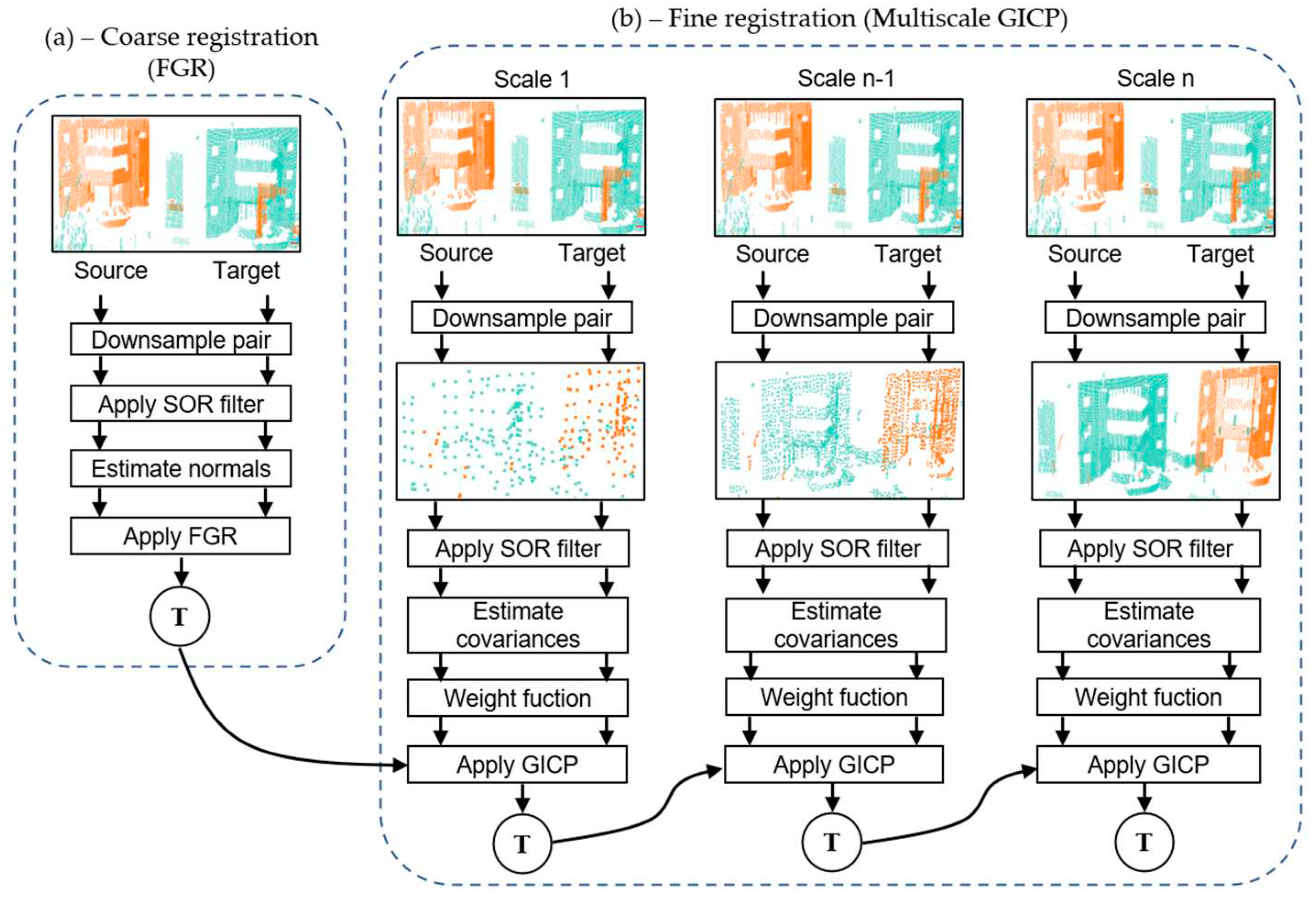
Figure 2.
(a) View of the Courtyard dataset. (b) View of the Façade dataset. (c) View of the NCLT dataset.
Figure 2.
(a) View of the Courtyard dataset. (b) View of the Façade dataset. (c) View of the NCLT dataset.

Figure 3.
Visual inspection of the registration of all pairs in the Courtyard dataset by the proposed model FGR+M-GICP.
Figure 3.
Visual inspection of the registration of all pairs in the Courtyard dataset by the proposed model FGR+M-GICP.
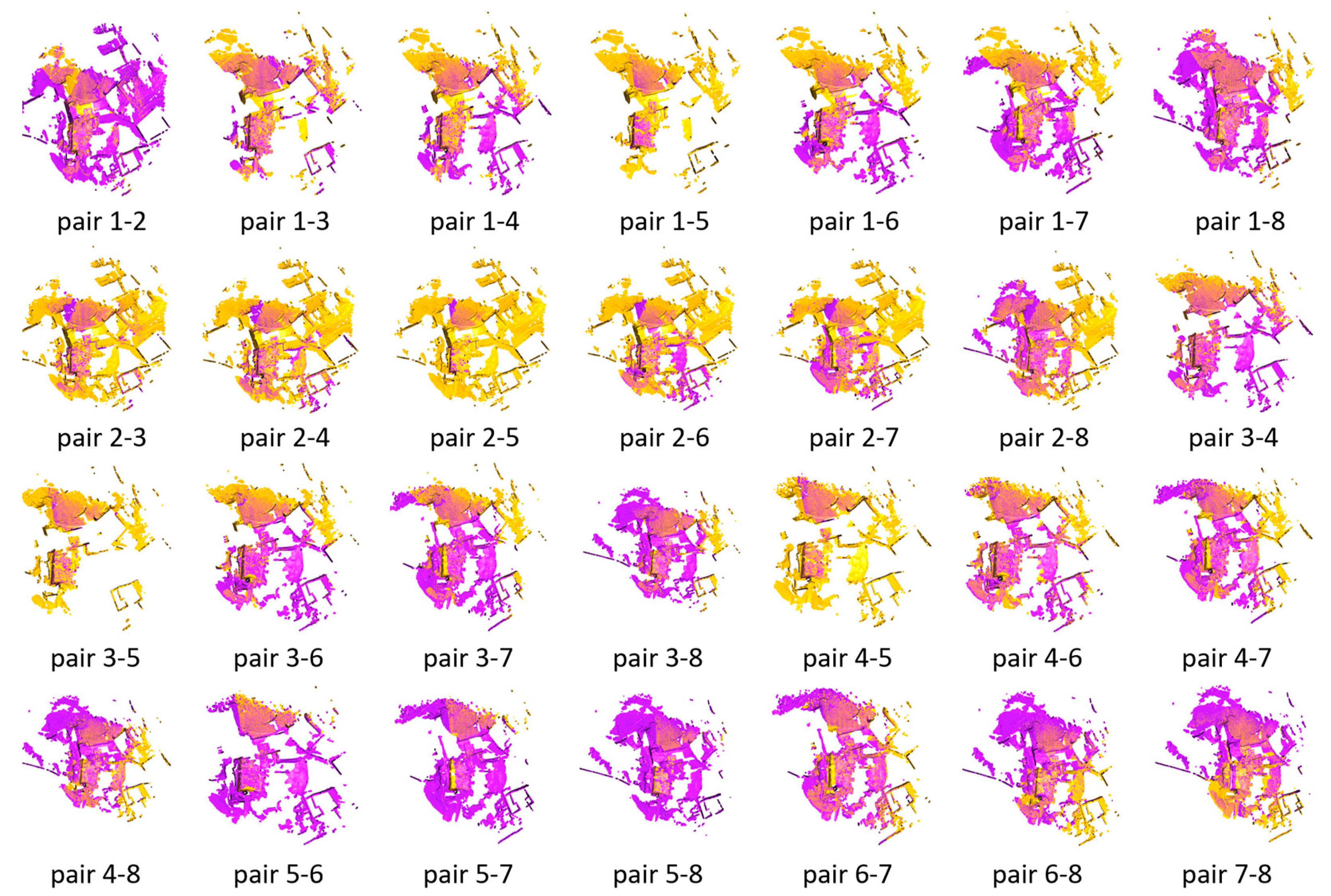
Figure 4.
RMSE of all the correspondences in the overlap area of each point cloud pair from the dataset Courtyard.
Figure 4.
RMSE of all the correspondences in the overlap area of each point cloud pair from the dataset Courtyard.
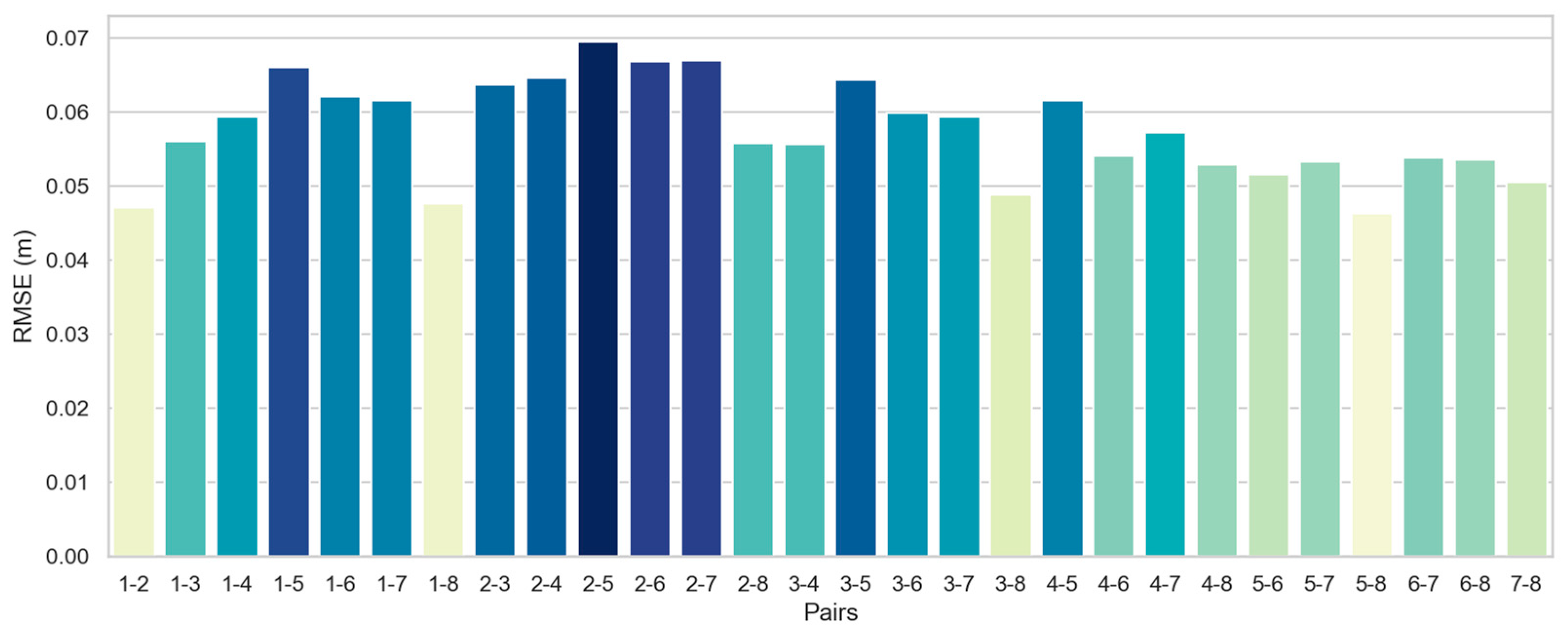
Figure 5.
Visual inspection of the registration of all pairs in the Facade dataset by the proposed model FGR+M-GICP.
Figure 5.
Visual inspection of the registration of all pairs in the Facade dataset by the proposed model FGR+M-GICP.
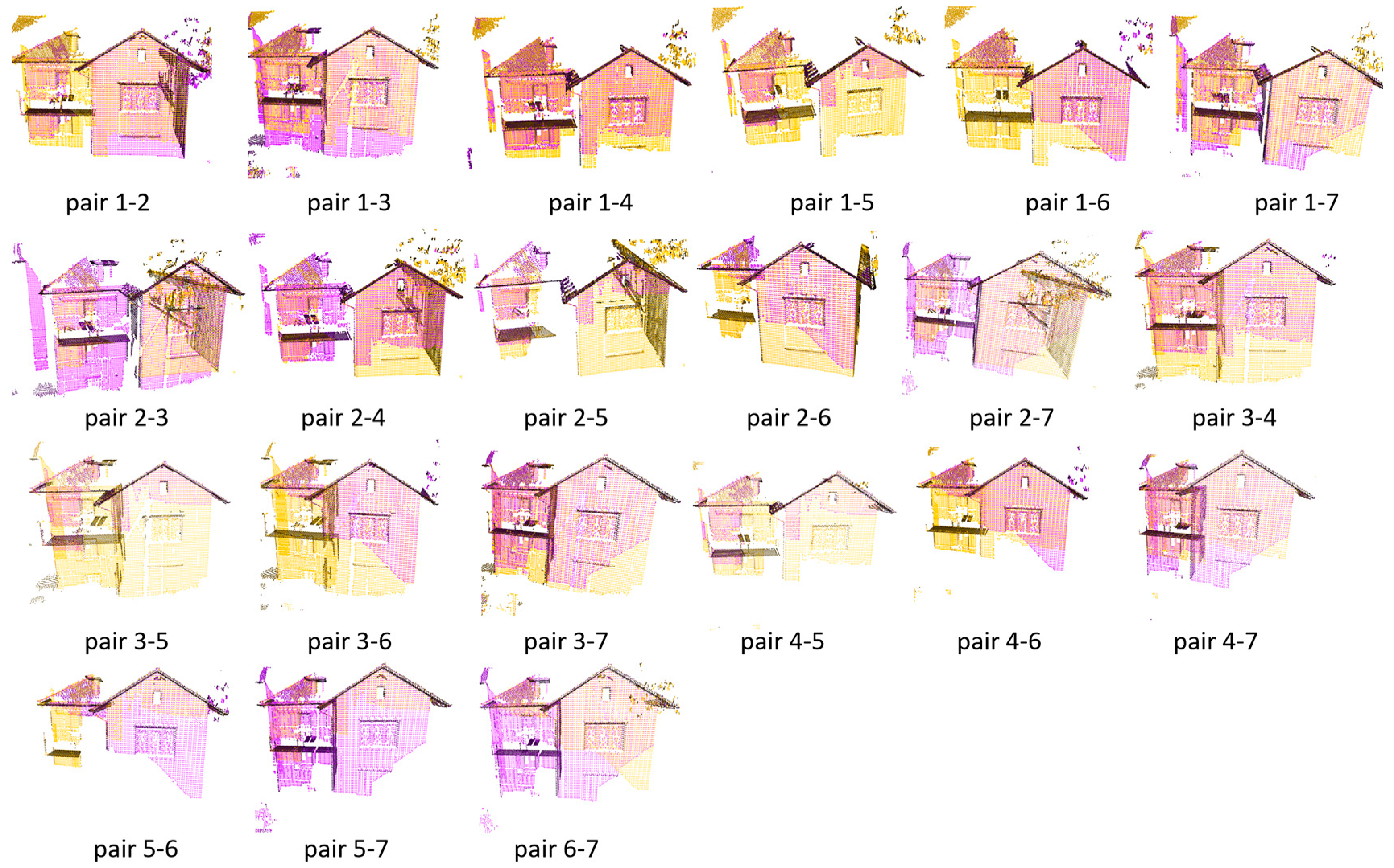
Figure 6.
RMSE of all the correspondences in the overlap area of each point cloud pair from the Facade dataset.
Figure 6.
RMSE of all the correspondences in the overlap area of each point cloud pair from the Facade dataset.
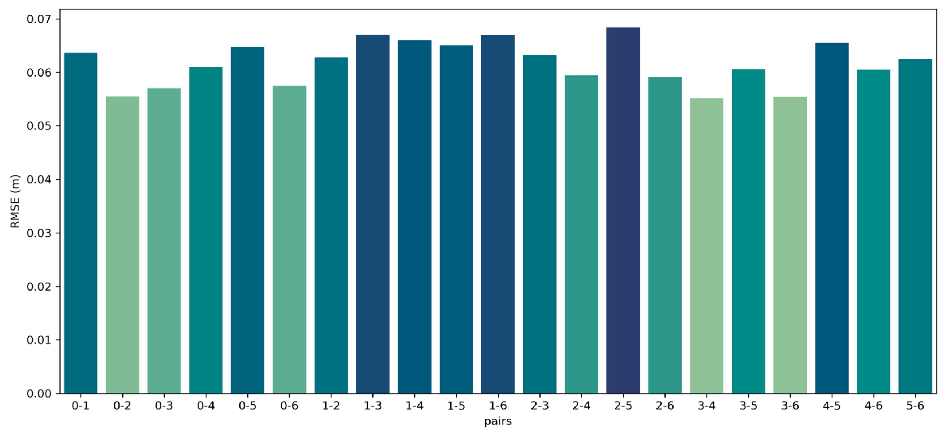
Figure 7.
A. Pair of point clouds 1-2 from the Facade dataset after registration with GICP Vanilla and M-GICP. Figure 7B. Multiscale downsampling voxels used in M-GICP. Figure 7C. RMSE over 250 iterations with 50 iterations per scale.
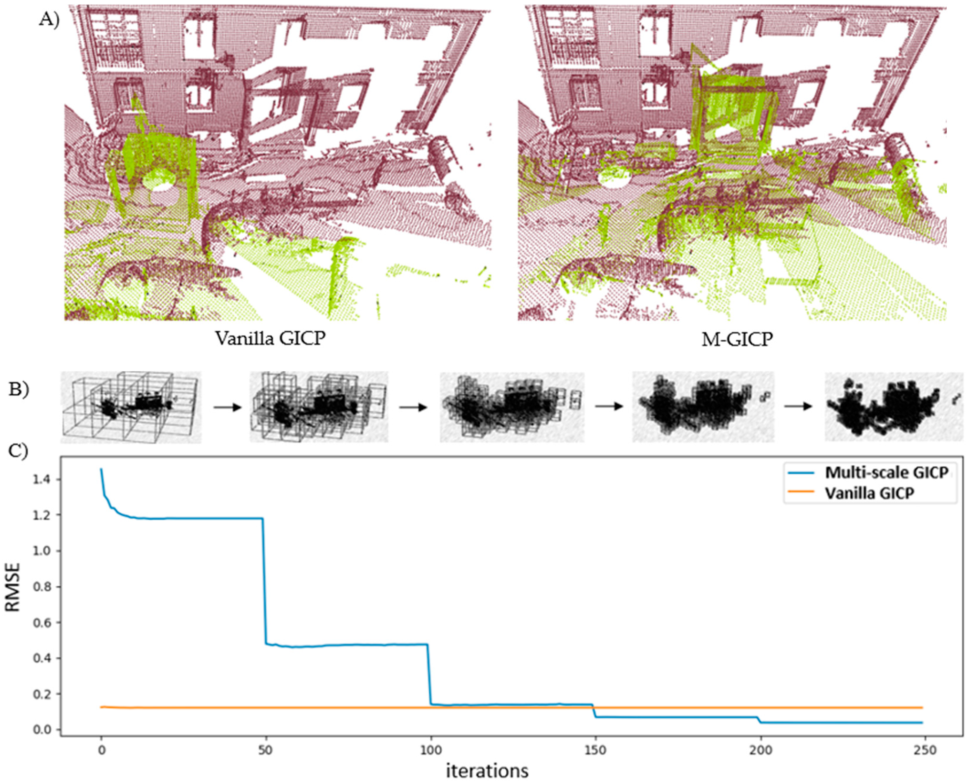
Figure 8.
A. LUM. Figure 8B. SLERP. Figure 8C. g2o. Figure 8D. SLERP+LUM (ours). Drift correction in the NCLT dataset.
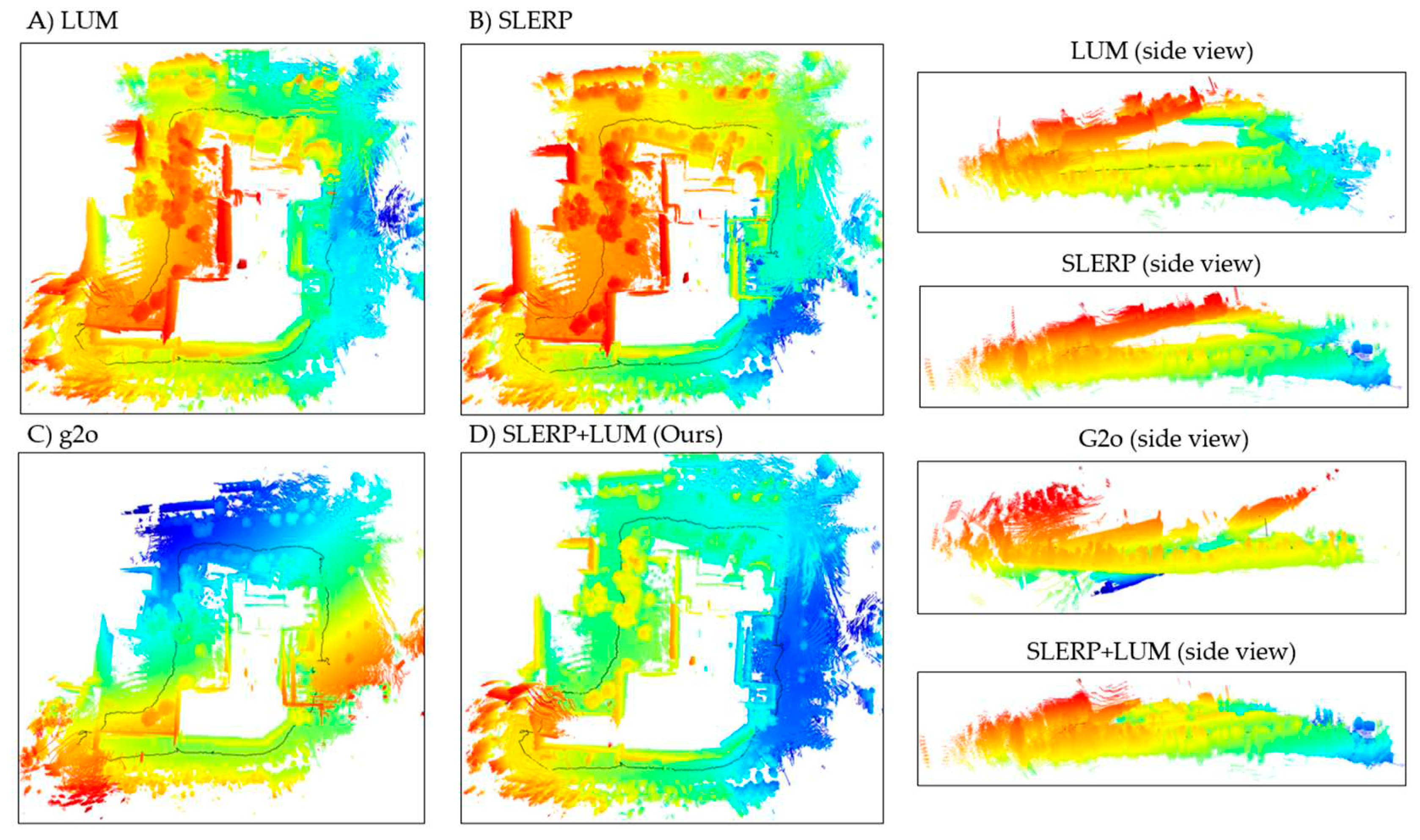
Figure 9.
Pose error of GRM models.

Figure 10.
Estimated trajectories with each of the MRGs and groundtruth. Figure 10A. Top view. Figure 10B. Side View.
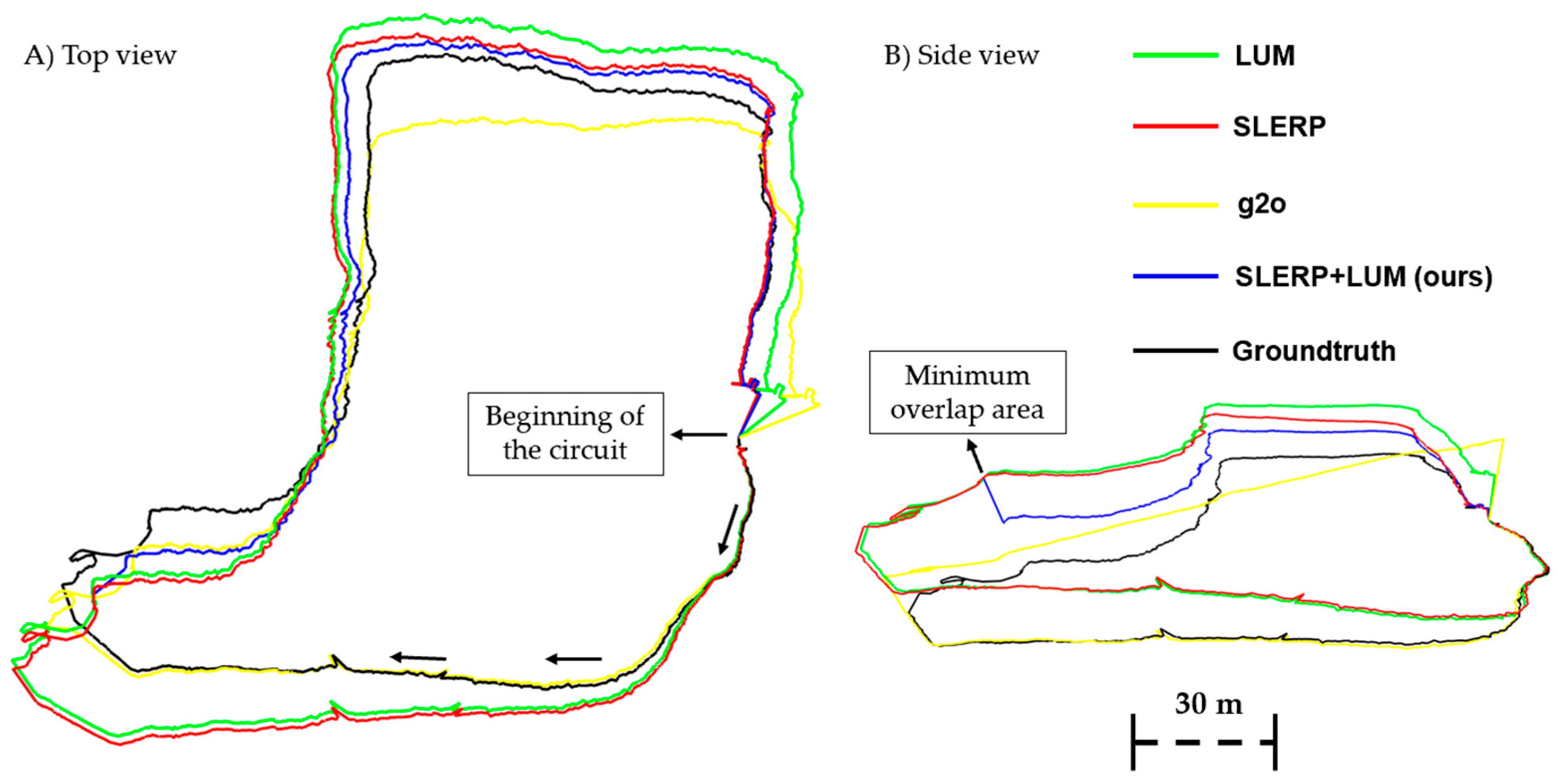
Figure 11.
Estimated time of execution of each GRM. Mean time of 100 executions.
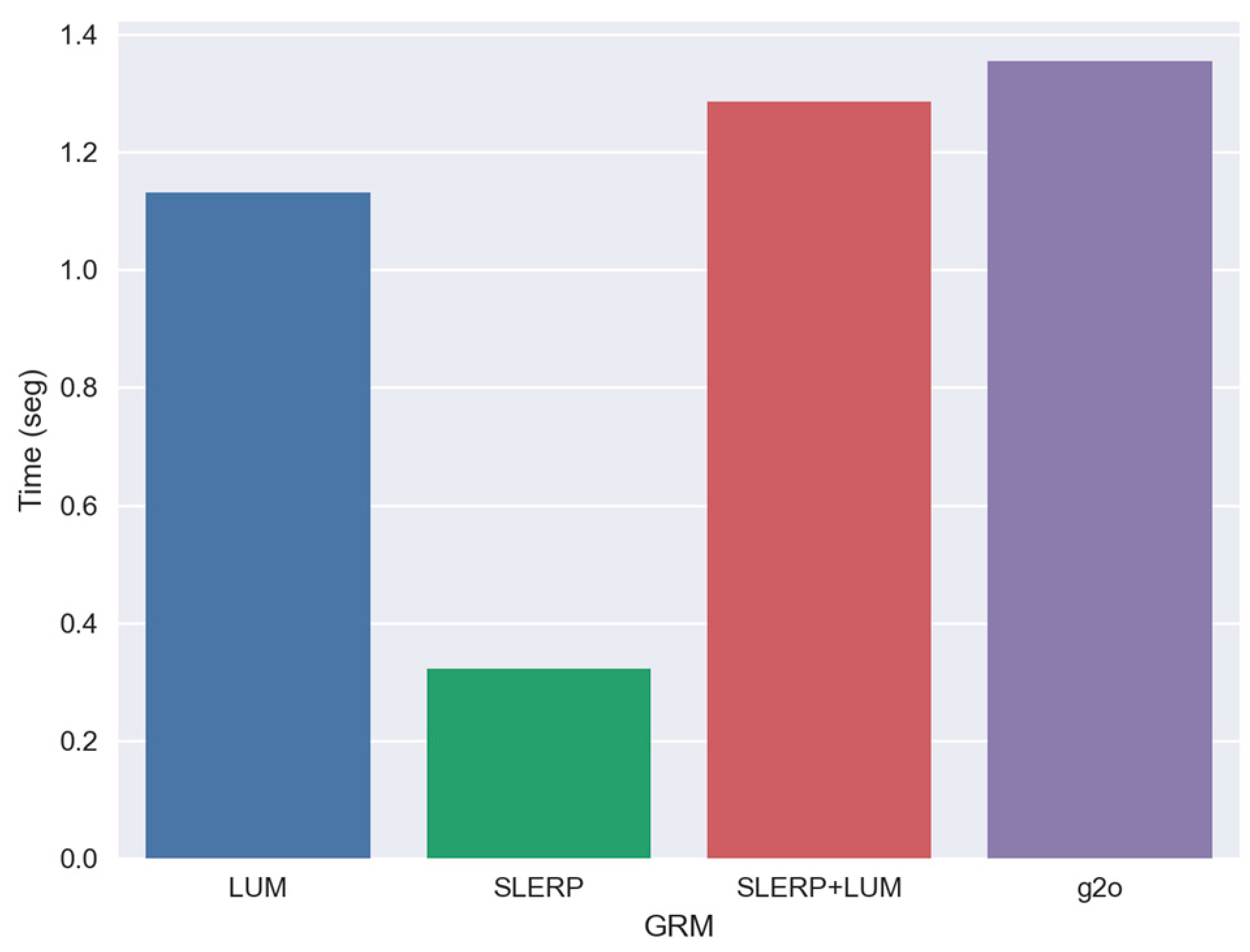
Table 1.
Parameters of FGR and Multiscale-GICP. knn = k-nearest-neighbors.
| Parameter | Value | Description |
|---|---|---|
| Voxel size | 0.1 for FGR [0.5; 0.4, 0.3, 0.2, 0.1] for M-GICP |
Used to reduce the number of points and uniformize the density along the point cloud pair |
| Maximum correspondence distance | 2 × voxel_size for FGR [3, 2.5, 2.0, 1.5, 1.0] × voxel_size for M-GICP |
Maximum distance to search for correspondences between source and target point cloud |
| Standard Deviation of SOR filter |
1.0 for FGR and 1.0 for all scales of M-GICP |
Used to filter the point cloud pair given a neighborhood |
| Neighborhood of the SOR filter | 30 knn for FGR 30 knn for all scales of M-GICP |
Number of neighbors used by the SOR filter |
| Neighborhood for normal estimation | 20 knn or 2 × voxel_size for FGR 20 knn or 2 × voxel_size for all scales of M-GICP |
Neighborhood used for normal estimation |
| Neighborhood for FPFH estimation | 200 knn or 10 × voxel_size | Neighborhood of the FPFH descriptor, we use a hybrid approach that can leverage a maximum radius or a value of knn. |
Disclaimer/Publisher’s Note: The statements, opinions and data contained in all publications are solely those of the individual author(s) and contributor(s) and not of MDPI and/or the editor(s). MDPI and/or the editor(s) disclaim responsibility for any injury to people or property resulting from any ideas, methods, instructions or products referred to in the content. |
© 2024 by the authors. Licensee MDPI, Basel, Switzerland. This article is an open access article distributed under the terms and conditions of the Creative Commons Attribution (CC BY) license (http://creativecommons.org/licenses/by/4.0/).
Copyright: This open access article is published under a Creative Commons CC BY 4.0 license, which permit the free download, distribution, and reuse, provided that the author and preprint are cited in any reuse.
MDPI Initiatives
Important Links
© 2024 MDPI (Basel, Switzerland) unless otherwise stated


