Submitted:
30 December 2023
Posted:
15 January 2024
You are already at the latest version
Abstract
Based on acoustic fluid elements, dynamic analysis was performed on liquid sloshing modes and liquid-filled containers considering the fluid-structure interaction (FSI) effect. The liquid sloshing modes in two-dimensional (2D) and three-dimensional (3D) containers were analyzed, and the results were compared with liquid sloshing modes measured in tests and theoretically calculated modes. This thus verifies correctness of the simulation method based on acoustic fluid elements. Cylindrical liquid-filled containers with different water levels were subjected to modal analysis and dynamic and time-historical analysis. Results show that the finite element analysis (FEA) based on acoustic fluid elements can accurately simulate liquid sloshing modes in liquid-filled containers and vibration characteristics of these containers with different liquid levels. The vibration frequency of liquid-filled containers declines obviously with rising liquid level. The liquid level significantly affects distributions of the maximum displacement, maximum acceleration, and maximum von Mises stress on the sidewall of liquid-filled containers. Numerical simulations based on acoustic fluid elements provides an effective and reliable method for dynamic analysis of liquid-filled containers considering the FSI effect.
Keywords:
fluid-structure interaction
; acoustic fluid elements
; liquid sloshing modes
; liquid-filled containers
; dynamic analysis
1. Introduction
The fluid-structure interaction (FSI) effect between solid structures and liquids is prevalent in practical engineering. For example, liquid-filled containers under seismic action or other vibration loads belong to one of structures with the typical FSI effect [1]. Analysis of the FSI effect of liquid-filled containers, on the one hand, focuses on liquid sloshing therein and on the other hand, considers the influence of liquid sloshing on these containers.
For liquid sloshing problems, Dodge et al. [2,3,4,5] systematically expounded the theoretical and engineering applications of liquid sloshing modes. However, these methods pay more attention to theoretical analytical methods and are only applicable to solving cases with regular shapes and simple external excitations while fail to solve vibration problems of liquid-filled structures of complex shapes [6,7]. Bao et al. [8,9] analyzed liquid modes based on potential-based fluid elements. When using the method, the liquid sloshing frequency is far lower than the structural vibration frequency and the obtained first hundreds of modes are all liquid sloshing modes rather than modes of solid structures [10]. Therefore, it is difficult to apply the mode-superposition response spectrum method and time history analysis to dynamic analysis of liquid-filled structures, and these methods are not applicable to analysis of dynamic responses of liquid-filled containers.
Structural engineers generally pay more attention to how liquid motion affects structural responses under seismic action, while they are not interested in the motion of liquids themselves. To consider the influence of liquid sloshing on dynamic responses of liquid-filled containers and avoid complex liquid sloshing computation, the simplified equivalent mechanical model of fluid sloshing is generally used. On the basis of the potential flow theory, Graham [11] took the lead to propose an equivalent mechanical model of fluid sloshing in a rectangular container, which has been widely applied in the engineering field. Housner [12] deduced the simplified calculation formula of equivalent model of fluids based on physical intuition analysis. Housner model is a good approximation for the exact solution to the model proposed by Graham and has found extensive applications to civil and hydraulic engineering. However, Housner model is not built based on physical intuition and therefore is not an exact physical model, so its results are not safe in some cases. Li [13] improved Housner model on the basis of the linear potential flow theory and provided the fitting solution to the equivalent model using a semi-analytical and semi-numerical method. Whereas, the improved Housner model has so complex parameters that it is only suitable for regular two-dimensional (2D) models while not to complex 2D and three-dimensional (3D) models. Apart from proposing the equivalent methods based on the potential flow theory, Wstergaard [14] and Chopra [15] also came up with the added mass method. Rajasankar et al. [16] applied the added mass method to the finite element method (FEM) and performed FSI analysis. Bao et al. [17] put forward the improved added mass model based on the added mass method and conducted dynamic analysis on an annular tank, providing reference for the design and application of annular tanks. However, the distributed mass coefficient is difficult to determine in the above added mass method and improved added mass methods, so when using these methods to analyze structures of liquid-filled containers, the results are generally less safe.
The conventional analytical methods are only applicable to cases with regular geometric shapes and simple external excitations, and FEM based on potential-based fluid elements is not applicable to analysis of dynamic responses of liquid-filled structures. Moreover, equivalent mechanical models based on fluid sloshing and the added mass methods also have drawbacks. Considering this, it is necessary to use a method that is not only suitable for analyzing liquid sloshing modes but also applicable to analyzing influences of liquid sloshing on dynamic responses of liquid-filled containers, so as to provide reference for engineering design and application of these containers. Therefore, the current research conducted finite element analysis (FEA) on liquid sloshing modes at first and compared the analysis results with theoretical solutions and liquid sloshing frequencies and modes measured in existing tests, thus verifying correctness of the FEM. Whereas, the theoretical solutions and test models are only applicable to 2D models, while practical models are all 3D ones, so 3D models of liquid sloshing were also analyzed. Then, dynamic analysis was performed on liquid-filled containers with different liquid levels, and influences of the FSI effect and the intrinsic frequency and dynamic response of liquid-filled containers were also considered. The FEM based on acoustic fluid elements used in the research provides an effective and reliable method for the dynamic analysis of liquid-filled containers considering the FSI effect.
2. FEA theory based on acoustic fluid elements
A liquid-filled container and a liquid constitute an FSI system, in which the liquid and structure (liquid-filled container) are simulated using FEM. The FEM simulation methods of structures have been introduced in detail in many monographs [18]. For FEA considering the FSI effect, one is to use the fluid displacement as an unknown quantity [19] and harness the similarity between the fluid motion equation and equation of motion of structural elastomers, which can obtain the finite element calculation model of fluid consistent with the finite element scheme; the other is to take the fluid pressure as an unknown quantity [20] and coordinate the displacement and pressure on the structure-fluid interface, from which the obtained mass and stiffness matrices are asymmetric matrices. When analyzing liquid sloshing problems using the pressure scheme based on acoustic fluid elements [21], the theory is described as follows:
For the structure:
where separately represent the mass, damping, and stiffness matrices of the structure; separately denote the acceleration, speed, and displacement vectors at nodes of structural elements; is the coupling matrix at the structure-fluid interface; is the nodal pressure vector of fluid elements; is the load vector of the structure.
For the fluid:
where separately represent the mass, damping, and stiffness matrices of the fluid; are the first-order and second-order derivatives of nodal pressure of fluid elements; is the fluid density; is the load vector of the fluid.
The following is obtained by combining Eqns. (8) and (9):
By solving Eq. (3), the liquid sloshing modes in the FSI system and the FSI dynamic responses can be obtained.
3. Analysis of liquid sloshing modes
3.1. Theoretical solutions to 2D liquid sloshing modes
Following the potential flow theory of ideal fluids, the fluid is assumed to be a non-viscous, irrotational, and incompressible ideal fluid, for which influence of the free surface tension of the liquid is not considered. For general practical engineering problems, the above assumption is feasible. By establishing the free sloshing equation for the liquid using the theoretical method, the corresponding eigenvalue equation is obtained. The liquid sloshing frequency and mode are attained by solving the eigenvalues.
1) 2D rectangular container
For a regular rectangular container (Figure 1a), the j-th sloshing frequency of the liquid is [2,3]:
where g is the gravitational acceleration; a is the half width of the rectangular container; h is the liquid level. According to Eq. (1), the sloshing of the free liquid surface is attributed to the gravity. The j-th sloshing mode of the free liquid surface is
where and are constants. Figure 2 illustrates the first six sloshing modes of the free liquid surface. Therein, odd-order frequencies correspond to the first three antisymmetric modes, while even-order frequencies correspond to the first three symmetric modes, respectively.
2) Container with arbitrary cross sections
An container of an arbitrary shape is displayed in Figure 1b, for which it is challenging to solve the theoretical solution due to the irregular boundary. Considering this, the Rize method is adopted to calculate the liquid sloshing frequency of containers in arbitrary shapes [22]:
where g is the gravitational acceleration; ; a is the half width of resting free liquid surface; is the liquid area.
3.2. FEA of 2D liquid sloshing modes
The model adopted is a flat container, through which the 2D liquid sloshing is simulated. The test models are illustrated in Figure 3. The water level and half width of the rectangular container are h = 0.12 m and a = 0.10 m; the water level and radius of the round container are h = 0.16 m and R = 0.125 m; and the radius, water level, and cavity thickness of the U-shaped container are R = 0.10 m, h = 0.115 m, and 20 mm, respectively [23].
In the FEA, the containers are assumed to be rigid bodies. Generally, containers are all elastomers, while the elastic vibration of containers only slightly influences the overall liquid sloshing, so the influence of stiffness of containers on liquid sloshing is ignored when analyzing liquid sloshing modes.
1) Rectangular container
The first four sloshing modes in the rectangular container obtained by FEA are shown in Figure 4; those measured in tests are displayed in Figure 5. It can be seen from Table 1 that the liquid sloshing frequency attained by FEA is consistent with the theoretical calculation results, with the maximum error within 0.5%. The maximum error in the sloshing frequency attained by FEA and that measured in tests is 3.1%. One of the causes for the error in the liquid sloshing frequency obtained using FEA and tests is that the liquid is assumed to be an ideal fluid in FEA, that is, incompressible fluid without viscosity, while the liquid in the tests is viscous. Besides, there is also an error in the test process, while the error is not large on the whole. Comparison of Figure 2 with Figure 4 and Figure 5 shows that the sloshing modes obtained by FEA agree well with the theoretically calculated modes, with a tiny difference only in the fourth order. The fourth sloshing modes obtained by FEA and tests are both even-order symmetric modes (Figure 2), so they are not different theoretically.
2) Round container
The first four liquid sloshing modes in the round container obtained by FEA are illustrated in Figure 6; those obtained in the tests are shown in Figure 7. Comparison shows that the sloshing modes obtained by FEA match well with those in the tests, with a tiny difference only in the second order. Whereas, the second modes are both symmetric modes, so they can be regarded consistent theoretically. Table 1 shows that the sloshing frequencies obtained by FEA are basically consistent with the first four sloshing frequencies attained by theoretical calculation, with the maximum error of 1.4%. The sloshing frequencies acquired by FEA have the maximum error of 5% with those measured in the tests, the source of which can refer to error analysis of the rectangular container.
3) U-shaped 2D container
The first four sloshing modes in the U-shaped 2D container attained by FEA are illustrated in Figure 8; while those measured in the tests are shown in Figure 9. Comparison shows that the sloshing modes attained by FEA are basically consistent with those measured in the tests, with a subtle difference only in the fourth order. Whereas, the fourth modes are both symmetric modes, which are regarded to have no difference theoretically. As displayed in Table 1, the sloshing frequencies acquired by FEA basically agree with the theoretically calculated first four frequencies, with an error smaller than 0.5%. The sloshing frequencies obtained by FEA and those measured in the tests have the maximum error of 2%, which indicates that the FEA results are reliable. The error analysis can refer to that of the rectangular container.
Based on the above analysis results, the liquid sloshing frequencies conform well to the theoretical calculation and test results, despite tiny differences in several modes. This indicates that the FEM based on acoustic fluid elements can well simulate the liquid sloshing modes in containers of different shapes.
3.3. FEA of 3D liquid sloshing modes
To compare with 2D models, the models of 3D containers remain to have the same geometric dimensions with 2D ones. The models are shown in Figure 10. For the cuboid container, the water level is h = 0.12 m, and its length and width are a = b = 0.20 m; the water level and radius of the spherical container are h = 0.16 m and R = 0.125 m; the water level and radius at the bottom of U-shaped 3D container are h = 0.115 m and R = 0.10 m, respectively.
1) Cuboid container
The liquid sloshing modes in the cuboid container obtained by FEA are shown in Figure 11 and Figure 12. Comparison of Figure 4 and Figure 11, combining with Table 1 and Table 2, shows that the first, third, sixth, and nineth liquid sloshing modes in the cuboid container separately correspond to the first, second, second, and fourth liquid sloshing modes in the rectangular container. The difference is that the liquid sloshing modes in the cuboid container are more complex than those in the rectangular container, and the frequencies are higher. It is more difficult to theoretically solve the liquid sloshing modes in the cuboid container than those in the rectangular container. Therefore, the FEM based on acoustic fluid elements can better simulate liquid sloshing modes in the cuboid container.
2) Spherical container
The liquid sloshing modes in the spherical container acquired by FEA are shown in Figure 13 and Figure 14. Comparison of Figure 6 and Figure 13, combining with Table 1 and Table 2, suggests that different from the cuboid and rectangular containers, the liquid sloshing modes in the spherical container do not correspond to those in the round container. This is because the length of the free liquid surface in the cuboid container (a = b = 0.20 m) remains identical to that in the rectangular container (a = 0.20 m), while the free liquid surface in the spherical container is not geometrically comparable to that in the round container.
3) U-shaped 3D container
The liquid sloshing modes in the U-shaped 3D container attained by FEA are shown in Figure 15 and Figure 16. By comparing Figure 8 and Figure 15 and combining with Table 1 and Table 2, it is found that the liquid sloshing modes in the U-shaped 3D container do not correspond to those in the U-shaped 2D container, while they are similar to those in the spherical container. This is because the free liquid surface in the U-shaped 3D container shows geometric similarity to that in the spherical container.
Comparison of liquid sloshing modes in 2D containers with those in 3D containers reveals that liquid sloshing modes in 3D containers are more complex than those in 2D containers, and the modes of the two do not correspond to each other. The FEM based on acoustic fluid elements can well simulate liquid sloshing modes in 2D and 3D containers of different shapes.
4. Modal analysis of cylindrical liquid-filled containers
4.1. Liquid modal analysis
For the cylindrical liquid-filled container in Figure 17, the liquid sloshing modes in elastic and rigid containers were analyzed separately. The model sizes and material parameters are listed in Table 3 [8].
The liquid sloshing frequency in the cylindrical liquid-filled container is [2,3]:
where is the i-th root of the derivative of the family of Bessel functions; g is the gravitational acceleration; R is the radius of the liquid-filled container; h is the liquid level in the liquid-filled container.
The first five liquid sloshing frequencies in the cylindrical liquid-filled container are listed in Table 4. The liquid sloshing modes in the cylindrical liquid-filled container and the vibration modes of this container are shown in Figure 18 and Figure 19, respectively. The FEA numerical solution conforms well to the theoretical solution, which indicates that it is highly reliable to simulate liquid sloshing modes in containers by using acoustic fluid elements. Moreover, the FEA results of liquid sloshing frequencies in rigid and elastic containers are same for this example, suggesting that the influence of structural stiffness on the liquid sloshing modes can be ignored.
4.2. Modal analysis of cylinder containers
In the practical engineering application, vibration frequencies of liquid-filled containers themselves attract more attention, in addition to liquid sloshing modes in liquid-filled containers. Therefore, it is necessary to analyze liquid-filled containers with different liquid levels.
The first five frequencies of liquid-filled containers with different liquid levels are displayed in Table 5. The results show that the liquid exerts great influences on the intrinsic frequency of cylindrical containers. As the liquid level rises in the liquid-filled containers, the vibration frequency of cylindrical containers declines obviously. If the liquid level in the liquid-filled containers is 6 m, the first frequency reduces by 31.24%. Therefore, the influences of the FSI effect on the intrinsic frequency and dynamic response of liquid-filled containers should be considered in the engineering design of these containers.
5. Dynamic and time-historical analysis of cylindrical liquid-filled containers
Cylindrical liquid-filled containers with different liquid levels were taken as examples to perform dynamic and time-historical analysis. The El-Centro (1940), Kobe (1995), and Loma Prieta (1989) waves were selected and applied in the x direction, with the peak acceleration of 0.1g. The acceleration time-history curves and Fourier spectra are shown in Figure 20. Structural analysis generally focuses on the displacement, acceleration, and stress of structures. Hence, the maximum displacement, maximum acceleration, and maximum von Mises stress on the sidewall at different heights of liquid-filled containers at x=D/2 and y=0 were monitored.
The distribution of the maximum displacement on the sidewall of containers with different liquid levels along the height is displayed in Figure 21. As the liquid level ascends, the maximum displacement on the sidewall of cylindrical liquid-filled containers constantly enlarges, while its location changes. When the liquid levels are 0 m (liquid-filled container not containing liquid), 1, and 2 m, the maximum displacement on the sidewall appears on the top of the container; under conditions with liquid levels of 3 and 4 m, the maximum displacement on the sidewall appears at the height of 2.5 m; if the liquid levels are 5 and 6 m, the maximum displacement on the sidewall occurs at the height of 3 m. The maximum displacement on the sidewall shares basically consistent distribution law along the height under conditions of different liquid levels and the three seismic waves, and they always increase on the sidewall of cylindrical liquid-filled container with rising liquid level. Whereas, the values of the maximum displacement are different. Taking the liquid level of 6 m as an example, the maximum displacements on the sidewall are separately 0.052, 0.049, and 0.046 mm under the El-Centro, Kobe, and Loma Prieta waves, and they all appear at the height of 3 m on the sidewall.
The distribution law of the maximum acceleration on the sidewall of containers with different liquid levels along the height is similar to that of the maximum displacement on the sidewall. It can be seen from Figure 21 that as the liquid level rises, the maximum acceleration on the sidewall of cylindrical liquid-filled containers constantly grows, while its location varies. In the case that the liquid levels are 0, 1, and 2 m, the maximum acceleration on the sidewall appears on the top of the liquid-filled container; if the liquid levels are 3 and 4 m, the maximum acceleration on the sidewall is found at the height of 2.5 m; when the liquid levels are 5 and 6 m, the maximum acceleration on the sidewall occurs at the height of 3 m.
Under action of the three seismic waves, the maximum acceleration on the sidewall of containers with different liquid levels basically has the same distribution along the height. The maximum acceleration on the sidewall of cylindrical liquid-filled container always increases with ascending liquid level. Taking the liquid level of 6 m as an example, the maximum accelerations on the sidewall are 0.46, 0.20, and 0.058 m/s2 under the El-Centro, Kobe, and Loma Prieta waves, respectively, and they all appear at the height of 3 m. Under action of different seismic waves, the maximum acceleration on the sidewall of containers with different liquid levels differs greatly in the distribution height. On the one hand, this is because the frequencies of input seismic waves differ greatly from the structural frequency. The main frequencies of the El-Centro, Kobe, and Loma Prieta waves all concentrate within 5 Hz (Figure 20). In the case of different liquid levels, the minimum and maximum first frequencies of the cylindrical container are 13.17 Hz (liquid level of 6 m) and 19.94 Hz (liquid level of 0 m), respectively. This suggests an unobvious acceleration amplification effect. On the other hand, El-Centro wave has more high-frequency spectra (higher than 15 Hz) compared with Kobe and Loma Prieta waves, so the maximum acceleration on the sidewall under the El-Centro wave is greater than those under Kobe and Loma Prieta waves.
The distribution of the maximum von Mises stress on the sidewall of containers with different liquid levels along the height is shown in Figure 23. The maximum von Mises stress is always found at the bottom of the liquid-filled containers. Apart from the bottom, the maximum von Mises stress on the sidewall of cylindrical liquid-filled containers constantly increases as the liquid level ascends. When the liquid levels are 0, 1, and 2 m, the maximum von Mises stress on the sidewall appears at the height of 1.0 m; if the liquid levels are 3 and 4 m, the maximum von Mises stress on the sidewall occurs at the height of 2.0 m; in the case that liquid levels are 5 and 6 m, the maximum von Mises stress on the sidewall occurs at the height of 2.5 m. Under action of the three seismic waves, the maximum von Mises stress on the sidewall shows basically consistent distribution law along the height of containers with different liquid levels. As the liquid level rises, the maximum von Mises stress on the sidewall of cylindrical liquid-filled containers enlarges while the values of the maximum von Mises stress are different. Taking the liquid level of 6 m as an example, under the El-Centro, Kobe, and Loma Prieta waves, the maximum von Mises stresses on the sidewall are separately 0.150, 0.144, and 0.135 MPa, and they are all found at the height of 2.5 m.
6. Conclusions
Dynamic analysis was performed on liquid sloshing modes in liquid-filled containers and the liquid-filled containers using the FEM based on acoustic fluid elements. The following conclusions are obtained:
(1) The liquid sloshing modes in 2D and 3D liquid-filled containers of regular shapes and arbitrary cross sections were analyzed and compared with theoretical solution and test results. The results reveal that the FEM based on acoustic fluid elements is highly applicable and reliable.
(2) The liquid level exerts significant influences on the intrinsic frequency of liquid-filled containers. As the liquid level in liquid-filled containers rises, the vibration frequency of cylindrical containers reduces obviously. When the liquid level in liquid-filled containers is 6 m, the first frequency declines by 31.24%. During engineering design of liquid-filled containers, the influence of the FSI effect on the intrinsic frequency of these containers should not be ignored. This suggests that the FEM based on acoustic fluid elements can well consider the effect.
(3) For the cylindrical liquid-filled container in the research, the liquid level basically does not influence the displacement, acceleration, and stress of liquid-filled containers under horizonal seismic action if the liquid level is low (within 2 m). As the liquid level ascends (3 to 6 m), the displacement, acceleration, and stress of liquid-filled containers enlarge significantly. The acceleration responses of liquid-filled containers are particularly significantly affected by spectral characteristics of seismic waves.
References
- Ju Rongchu, Zeng Xinchuan, Coupled vibration theory of elastic structures and liquids, Seismological Press: Beijing, China, 1983. (In Chinese)
- Dodge F, T. The New Dynamic Behavior of Liquids in Moving Containers [R]. San Antonio, TX: Southwest Research Institute, 2000.
- Abramson H, N. The Dynamic Behavior of Liquids in Moving Containers. NASA SP-106[J]. NASA Special Publication, 1966, 106.
- Ibrahim R, A. Liquid sloshing dynamics: theory and applications [M]. Cambridge: Cambridge University Press, 2005.
- Faltinsen O M, Timokha A N. Sloshing [M]. Cambridge: Cambridge University Press, 2009.
- Wang Jianjun, Li Qihan, Zhu Zigen, A Review of Numerical Methods For Fluid-structure Interaction with Large Free Surface Sloshing, Chinese Quarterly of Mechanics, 2001, (04):447-454. (In Chinese)
- Wen Dechao, Zheng Zhaochang, Sun Huanchun, Development of aseismic research on liquid storage tanks, Advances in Mechanics, 1995, (01):60-76. (In Chinese)
- Bao Xin, Liu Jingbo, Dynamic Finite Element Analysis Methods for Liquid Container Considering Fluid-Structure Interaction, Nuclear Power Engineering, 2017, 38(02):111-114. (In Chinese)
- Tan Xiaojing, Seismic response analysis of fluid-structure interaction of large liquid storage tank, Institute of Engineering Mechanics, China Earthquake Administration, 2008. (In Chinese)
- Xu Gang, Ren Wenmin, Zhang Wei, et al. Dynamic characteristic analysis of liquid-filled tanks as a 3-d fluid-structure coupling system, Chinese Journal of Theoretical and Applied Mechanics, 2004, (03):328-335. (In Chinese)
- Graham E W, Rodriguez A M. The characteristics of fuel motion which affect airplane dynamics [J]. Journal of Applied Mechanics, 1952, 19(3):381-388.
- Yuchun, Li, and, et al. A supplementary, exact solution of an equivalent mechanical model for a sloshing fluid in a rectangular tank [J].Journal of Fluids and Structures, 2012, 31(1):147-151.
- Housner G, W. Earthquake pressures on fluid containers [R]. Pasadena, California: California Institute of Technology, 1954: 1-39.
- H. M. Westergaard, M. ASCE. Water Pressures on Dams during Earthquakes [J]. Transactions of the American Society of Civil Engineers, 1933, Vol. 98(2): 418-432.
- Hall J F, Chopra A K. Hydrodynamic effects in the dynamic response of concrete gravity dams [J]. Earthquake Engineering & Structural Dynamics, 1982, 10(2):333-345.
- Rajasankar J, Iyer N R, Rao T V S R A. A new 3-D finite element model to evaluate added mass for analysis of fluid-structure interaction problems [J]. International Journal for Numerical Methods in Engineering, 1993, 36(6):997-1012.
- Bao Xin, Liu Jingbo, Yang Yue, Comparative study on added mass methods for dynamic analysis of annular water tank in nuclear engineering, Journal of Building Structures, 2018, 39(09):130-139. (In Chinese)
- Wang Xucheng, Finite element method, Tsinghua University Press: Beijing, China, 2003. (In Chinese)
- Chen H C, Taylor R L. Vibration analysis of fluid-solid systems using a finite element displacement formulation [J]. International Journal for Numerical Methods in Engineering, 1990, 29(4):683-698.
- G. C, Everstine. Finite element formulations of structural acoustics problems [J]. Computers & Structures, 1997, 65(3):307-321.
- Acoustic Analysis Guide Release 2023 R2, ANSYS, Inc., 2023.
- Li Y, Wang Z. An Approximate Analytical Solution of Sloshing Frequencies for a Liquid in Various Shape Aqueducts [J]. Shock and Vibration, 2014, (2014-2-13), 2014, 2014(pt.1):118-124.
- Li, YC; Wang, Z. Unstable characteristics of two-dimensional parametric sloshing in various shape tanks: theoretical and experimental analyses [J]. Journal of Vibration and Control, 2016, Vol.22 19): 4025-4046.
- Li Yuchun, Fundamentals of fluid sloshing dynamics, Science Press, 2017.
Figure 1.
Liquid in 2D containers. (a) Rectangular container; (b) Container with an arbitrary cross section.
Figure 1.
Liquid in 2D containers. (a) Rectangular container; (b) Container with an arbitrary cross section.
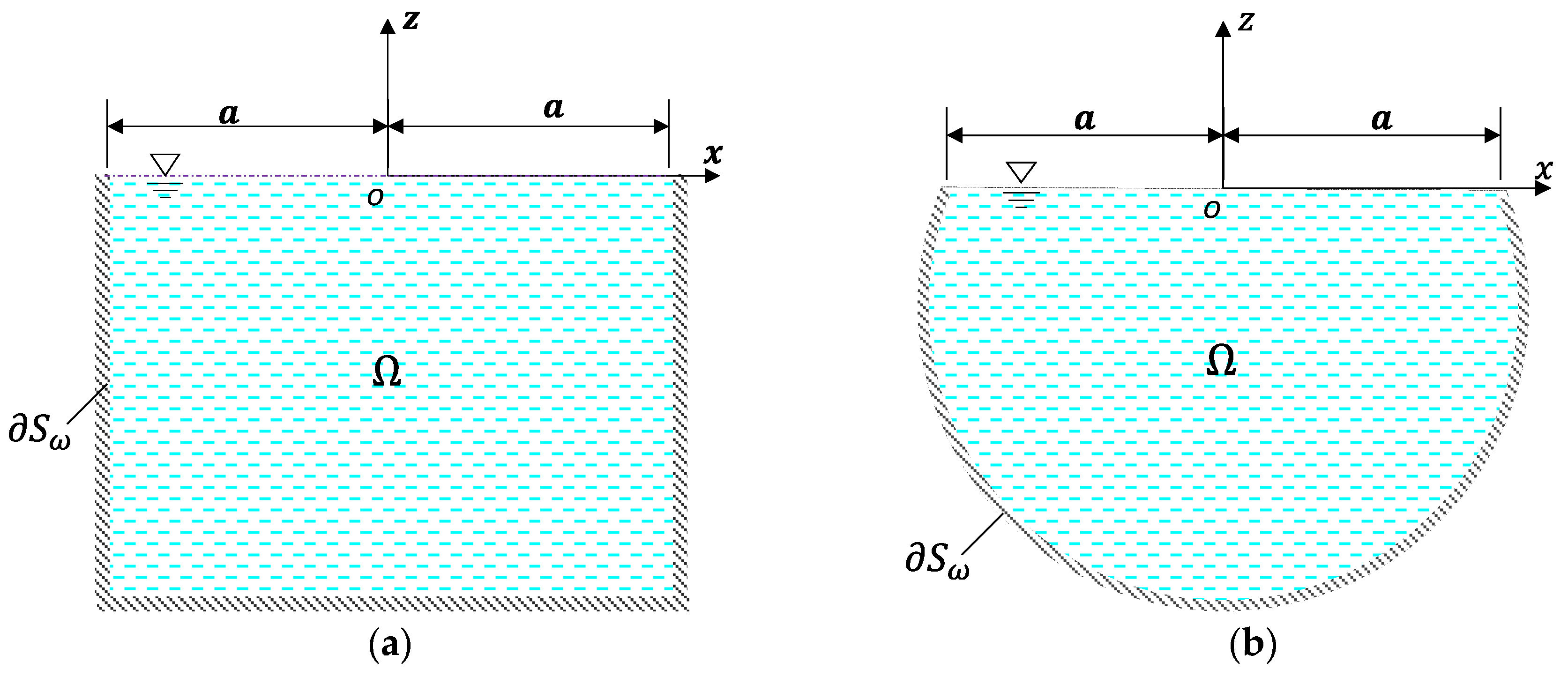
Figure 2.
The first six sloshing modes of the free liquid surface in the rectangular container.
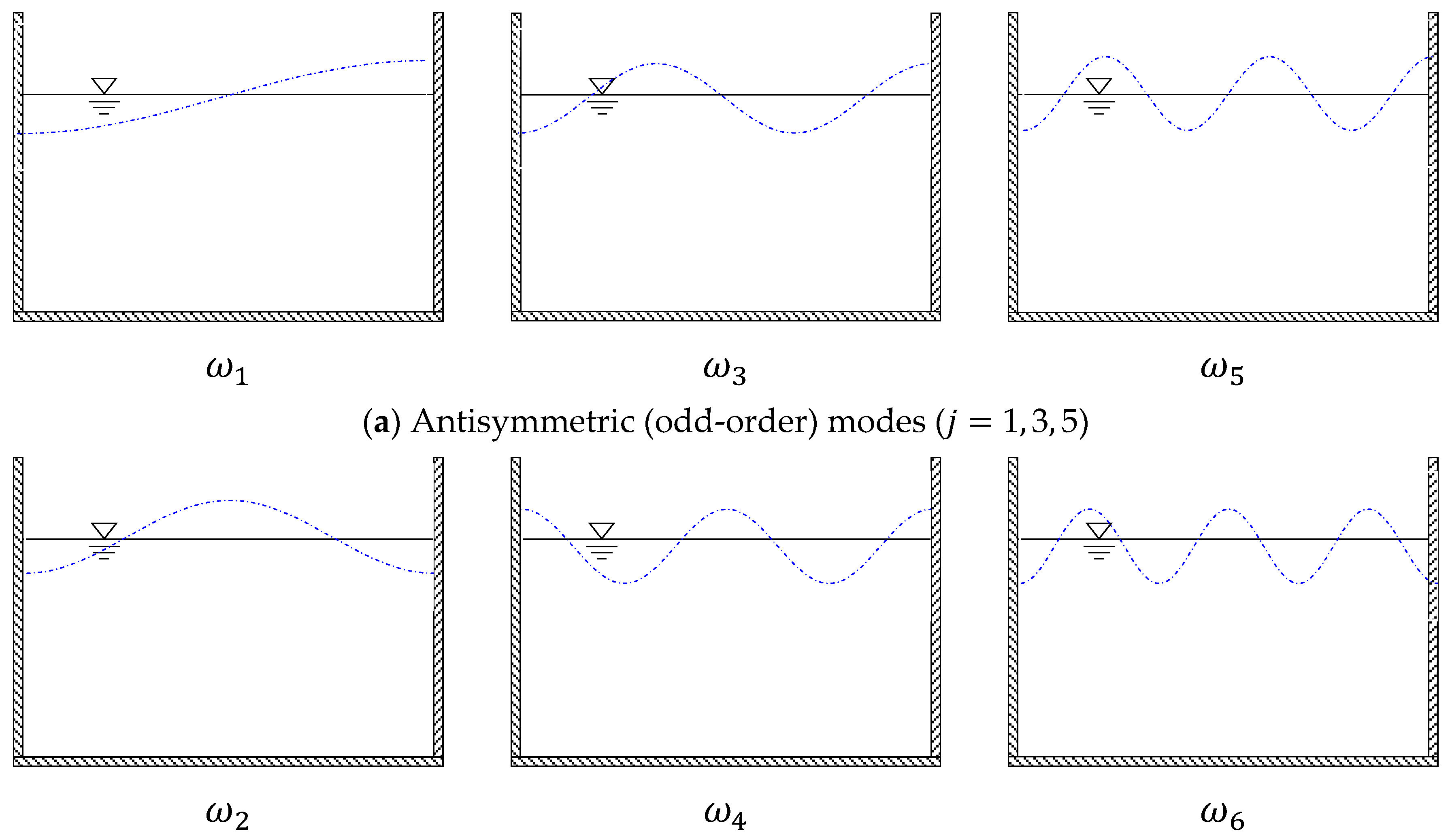
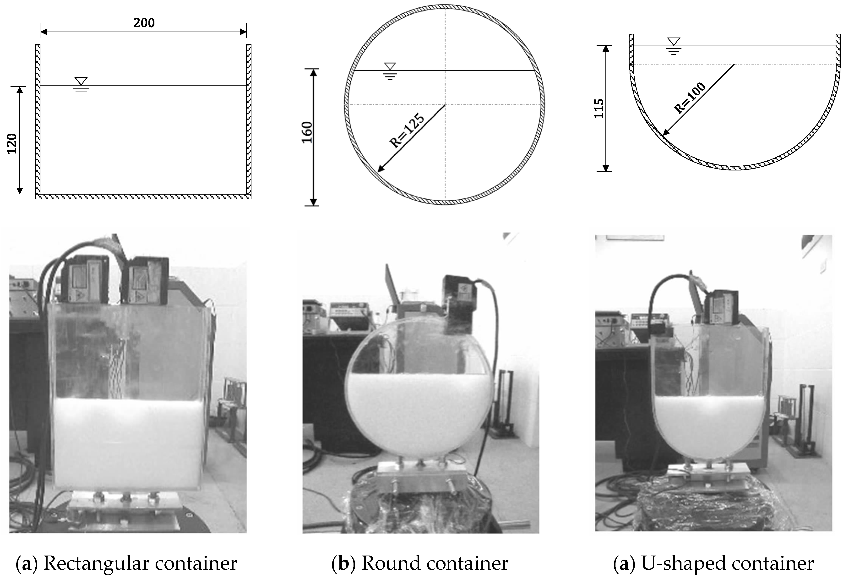
Figure 4.
The first four liquid sloshing modes in the rectangular container obtained by FEA. (a) The first order; (b) The second order; (c) The third order; (d) The fourth order.
Figure 4.
The first four liquid sloshing modes in the rectangular container obtained by FEA. (a) The first order; (b) The second order; (c) The third order; (d) The fourth order.
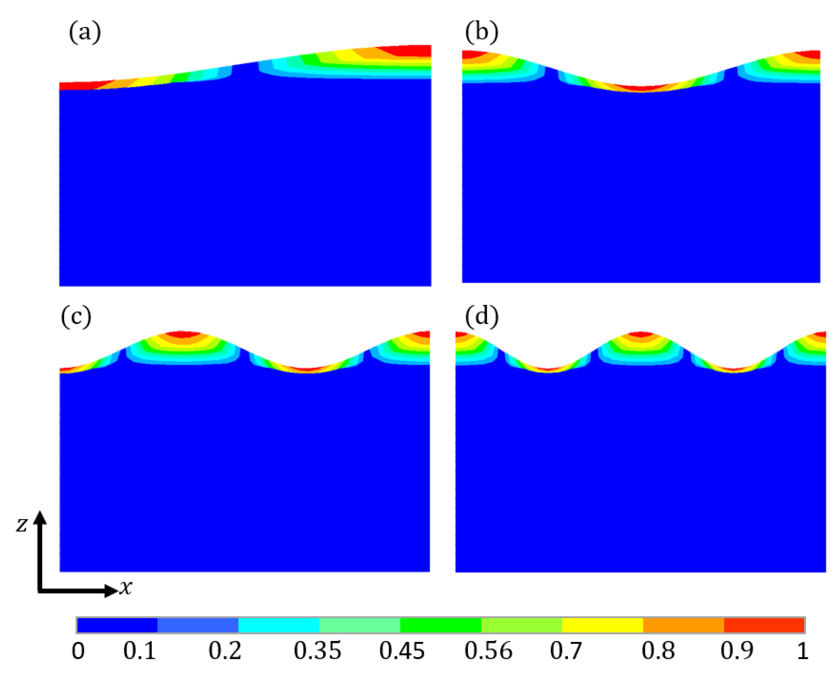
Figure 5.
The first four liquid sloshing modes in the rectangular container measured in the tests [23,24]. (a) The first order; (b) The second order; (c) The third order; (d) The fourth order.

Figure 6.
The first four liquid sloshing modes in the round container obtained by FEA. (a) The first order; (b) The second order; (c) The third order; (d) The fourth order.
Figure 6.
The first four liquid sloshing modes in the round container obtained by FEA. (a) The first order; (b) The second order; (c) The third order; (d) The fourth order.
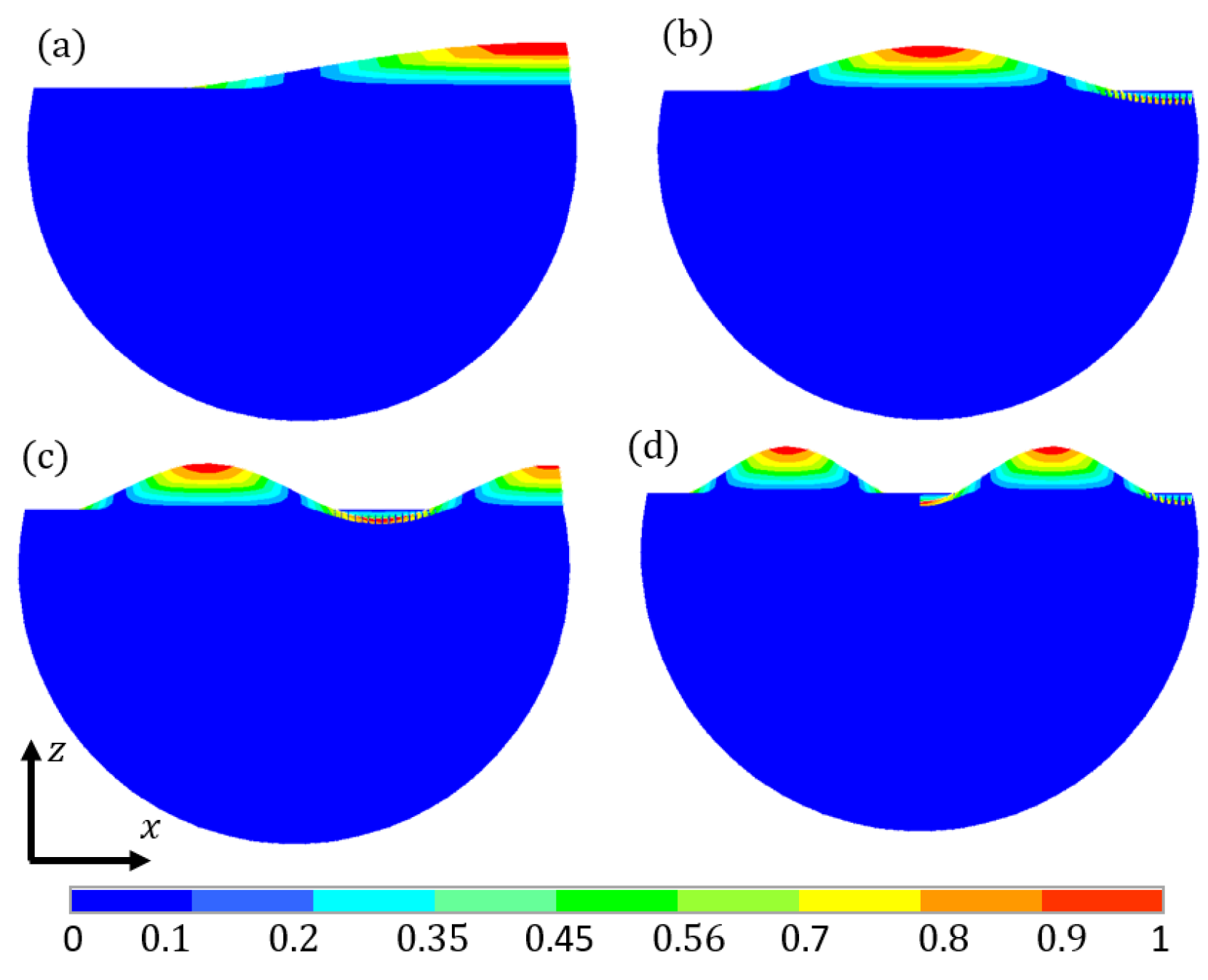
Figure 7.
The first four liquid sloshing modes in the round container measured in the tests [23,24]. (a) The first order; (b) The second order; (c) The third order; (d) The fourth order.
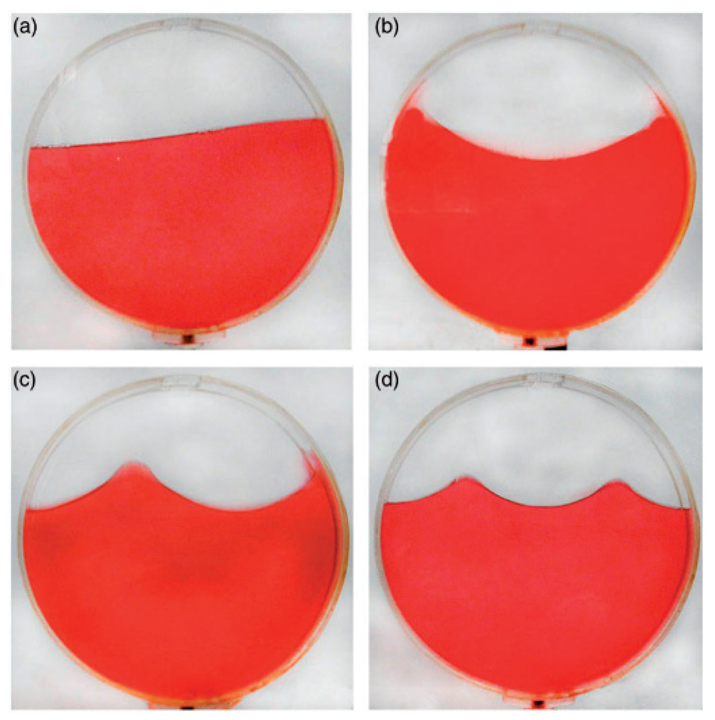
Figure 8.
The first four liquid sloshing modes in the U-shaped 2D container obtained by FEA. (a) The first order; (b) The second order; (c) The third order; (d) The fourth order.
Figure 8.
The first four liquid sloshing modes in the U-shaped 2D container obtained by FEA. (a) The first order; (b) The second order; (c) The third order; (d) The fourth order.
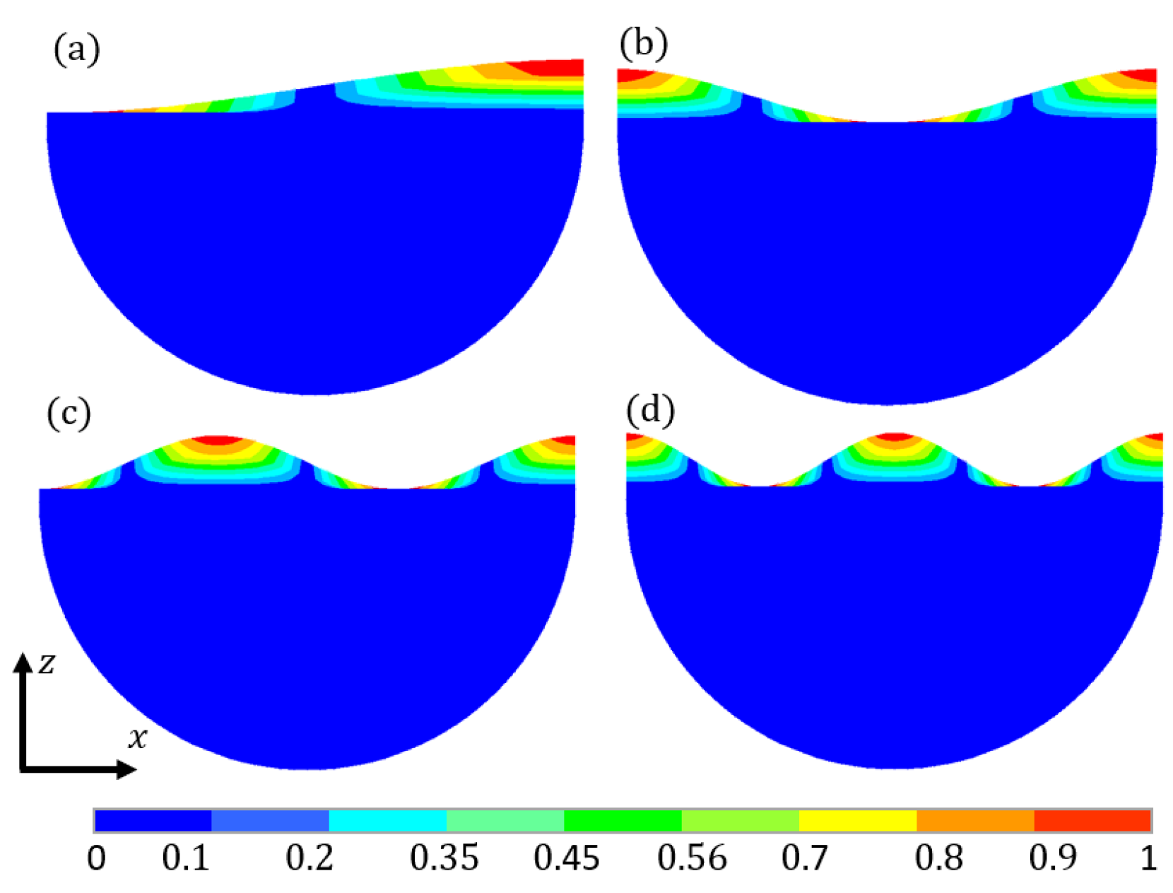
Figure 9.
The first four liquid sloshing modes in the U-shaped 2D container measured in the tests [23,24]. (a) The first order; (b) The second order; (c) The third order; (d) The fourth order.
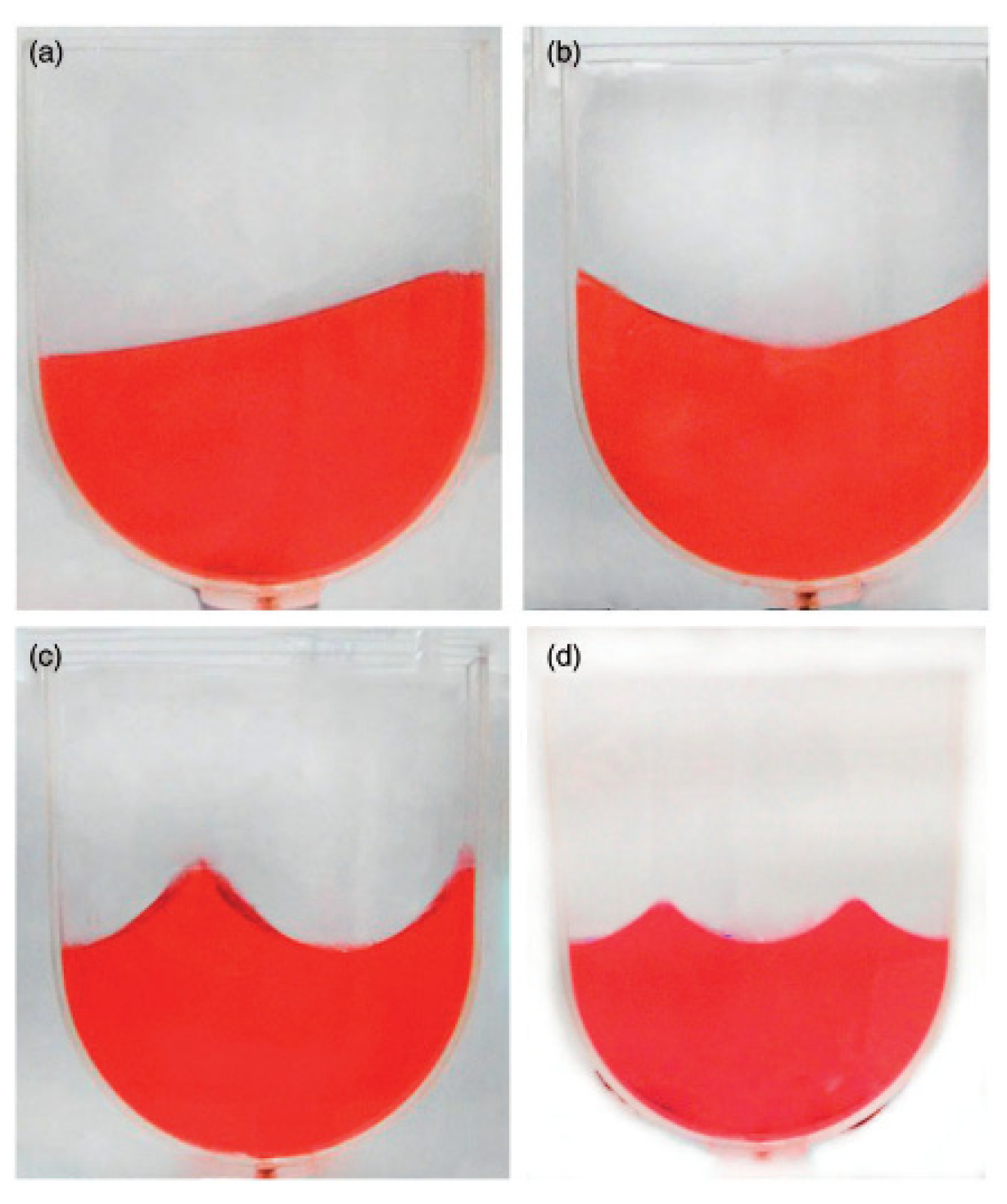
Figure 10.
3D liquid sloshing models.
Figure 11.
2D view of liquid sloshing modes in the cuboid container obtained by FEA. (a) The first order; (b) The third order; (c) The sixth order; (d) The nineth order.
Figure 11.
2D view of liquid sloshing modes in the cuboid container obtained by FEA. (a) The first order; (b) The third order; (c) The sixth order; (d) The nineth order.
Figure 12.
3D view of liquid sloshing modes in the cuboid container obtained by FEA. (a) The first order; (b) The third order; (c) The sixth order; (d) The nineth order.
Figure 12.
3D view of liquid sloshing modes in the cuboid container obtained by FEA. (a) The first order; (b) The third order; (c) The sixth order; (d) The nineth order.
Figure 13.
2D view of liquid sloshing modes in the spherical container obtained by FEA. (a) The first order; (b) The second order; (c) The third order; (d) The fourth order.
Figure 13.
2D view of liquid sloshing modes in the spherical container obtained by FEA. (a) The first order; (b) The second order; (c) The third order; (d) The fourth order.
Figure 14.
3D view of liquid sloshing modes in the spherical container obtained by FEA. (a) The first order; (b) The second order; (c) The third order; (d) The fourth order.
Figure 14.
3D view of liquid sloshing modes in the spherical container obtained by FEA. (a) The first order; (b) The second order; (c) The third order; (d) The fourth order.
Figure 15.
2D view of liquid sloshing modes in the U-shaped 3D container obtained by FEA. (a) The first order; (b) The second order; (c) The third order; (d) The fourth order.
Figure 15.
2D view of liquid sloshing modes in the U-shaped 3D container obtained by FEA. (a) The first order; (b) The second order; (c) The third order; (d) The fourth order.
Figure 16.
3D view of liquid sloshing modes in the U-shaped 3D container obtained by FEA. (a) The first order; (b) The second order; (c) The third order; (d) The fourth order.
Figure 16.
3D view of liquid sloshing modes in the U-shaped 3D container obtained by FEA. (a) The first order; (b) The second order; (c) The third order; (d) The fourth order.
Figure 17.
Cylindrical liquid-filled containers: H-Container height; D-Container diameter; t-Container wall thickness; h-Liquid level.
Figure 17.
Cylindrical liquid-filled containers: H-Container height; D-Container diameter; t-Container wall thickness; h-Liquid level.
Figure 18.
Liquid sloshing modes in the cylindrical liquid-filled container. (a) The first order; (b) The second order; (c) The third order; (d) The fourth order.
Figure 18.
Liquid sloshing modes in the cylindrical liquid-filled container. (a) The first order; (b) The second order; (c) The third order; (d) The fourth order.
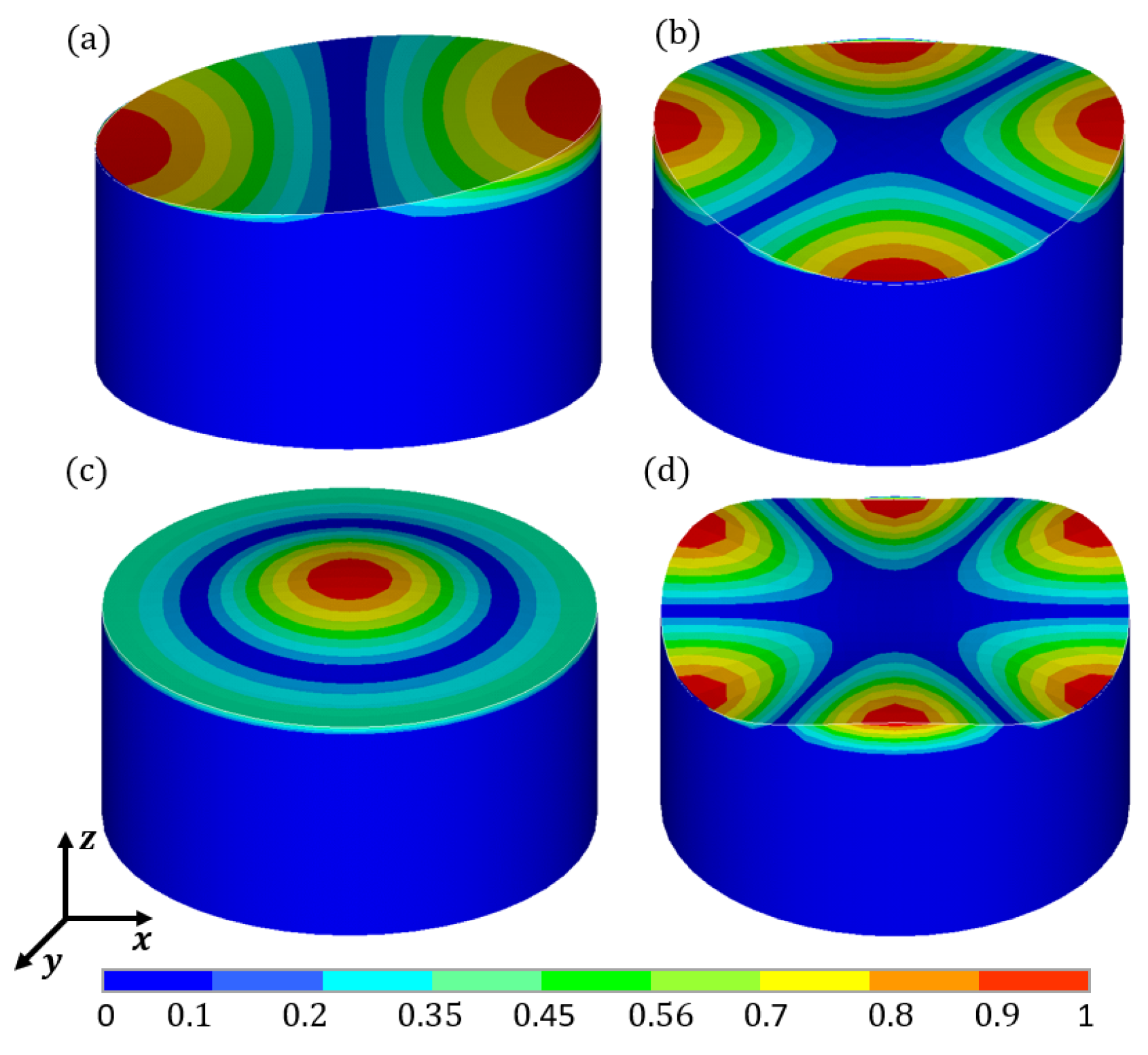
Figure 19.
Vibration modes of the cylindrical liquid-filled container. (a) The first order; (b) The second order; (c) The third order; (d) The fourth order.
Figure 19.
Vibration modes of the cylindrical liquid-filled container. (a) The first order; (b) The second order; (c) The third order; (d) The fourth order.
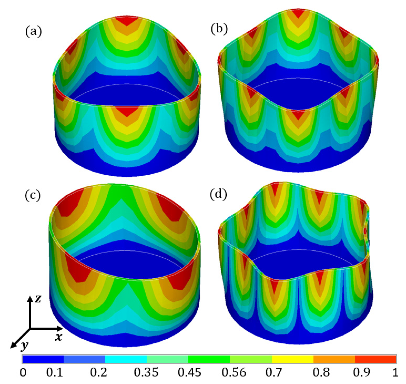
Figure 20.
Acceleration time-history curves and Fourier spectra under seismic waves.

Figure 21.
Distribution of the maximum displacement on the sidewall of containers with different liquid levels along the height.
Figure 21.
Distribution of the maximum displacement on the sidewall of containers with different liquid levels along the height.
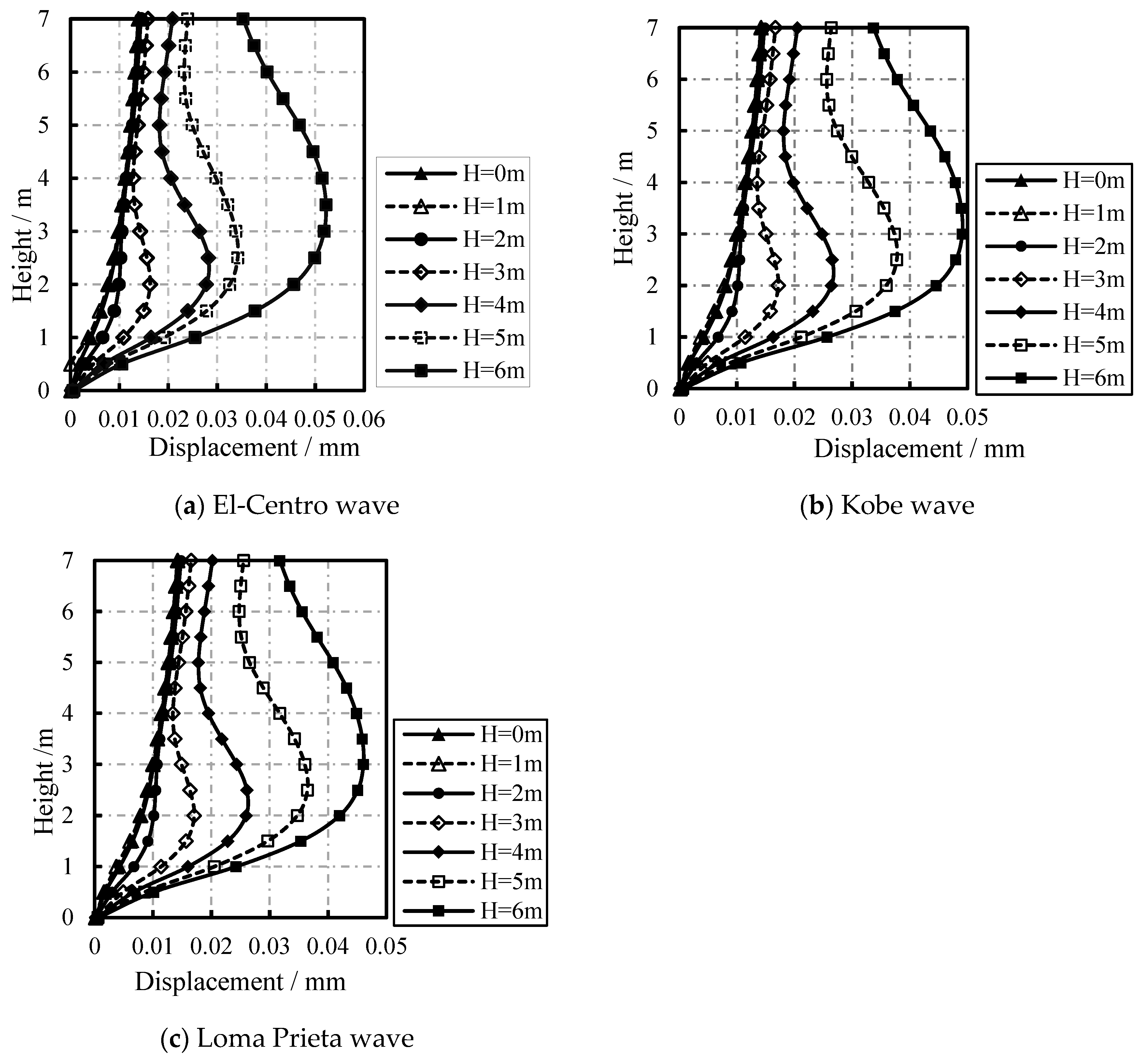
Figure 22.
Distribution of the maximum acceleration on the sidewall of containers with different liquid levels along the height.
Figure 22.
Distribution of the maximum acceleration on the sidewall of containers with different liquid levels along the height.
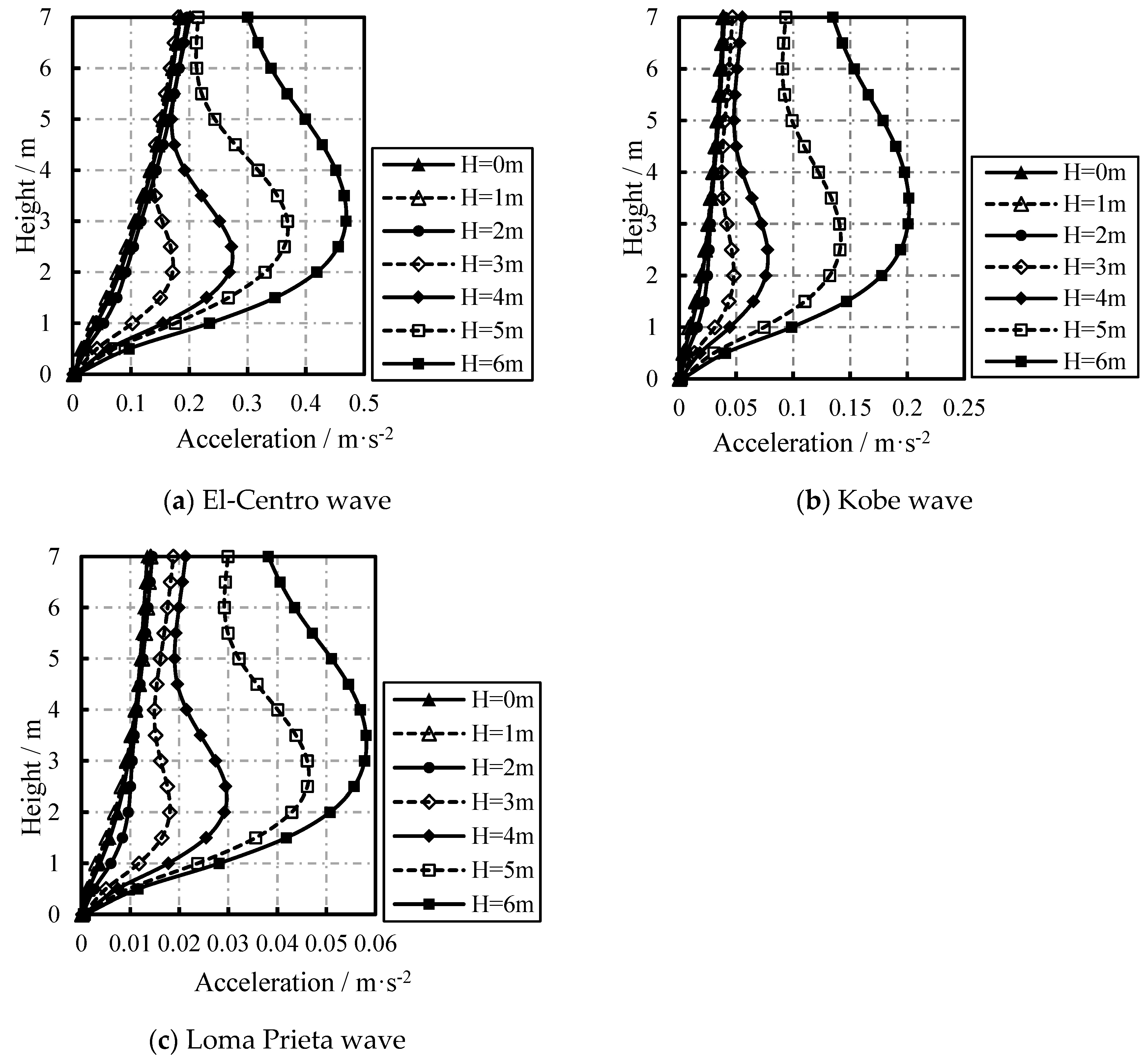
Figure 23.
Distribution of the maximum von Mises stress on the sidewall of containers with different liquid levels along the height.
Figure 23.
Distribution of the maximum von Mises stress on the sidewall of containers with different liquid levels along the height.
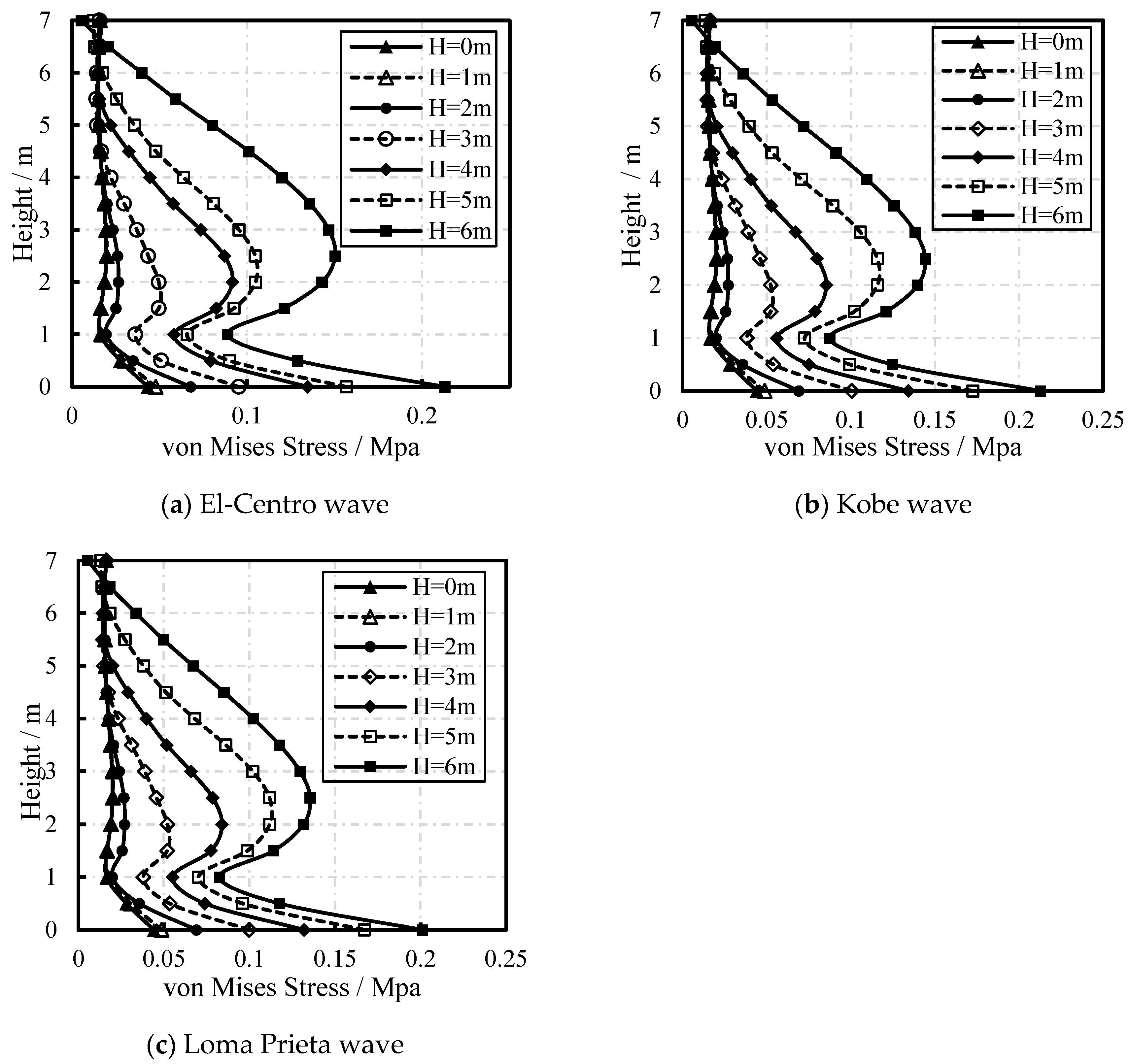

Table 1.
Comparison of the first four order frequency in FEA, theoretical analysis, and tests (Unit: Hz).
Table 1.
Comparison of the first four order frequency in FEA, theoretical analysis, and tests (Unit: Hz).
| Order | Rectangular container Water level h = 0.12 m |
Round container Water level h = 0.16 m |
U-Shaped container Water level h = 0.115 m |
||||||
| Theoretical calculation | Test | FEA | Theoretical calculation | Test | FEA | Theoretical calculation | Test | FEA | |
| 1 | 1.93 | 1.89 | 1.93 | 1.77 | 1.68 | 1.77 | 1.90 | 1.85 | 1.89 |
| 2 | 2.79 | 2.73 | 2.79 | 2.55 | 2.52 | 2.57 | 2.78 | 2.73 | 2.78 |
| 3 | 3.42 | 3.40 | 3.43 | 3.12 | 3.09 | 3.15 | 3.42 | 3.35 | 3.42 |
| 4 | 3.95 | 3.94 | 3.97 | 3.61 | 3.51 | 3.64 | 3.95 | 3.87 | 3.95 |
Table 2.
The first ten liquid sloshing frequencies in different types of liquid-filled containers (Unit: Hz).
Table 2.
The first ten liquid sloshing frequencies in different types of liquid-filled containers (Unit: Hz).
| Container | Order | |||||||||
| 1 | 2 | 3 | 4 | 5 | 6 | 7 | 8 | 9 | 10 | |
| Cuboid container (Water level h = 0.12 m) |
1.93 | 2.34 | 2.80 | 2.97 | 3.34 | 3.45 | 3.55 | 3.79 | 4.01 | 4.08 |
| Spherical container (Water level h = 0.16 m) |
1.95 | 2.57 | 2.85 | 3.04 | 3.37 | 3.44 | 3.79 | 3.80 | 3.88 | 4.12 |
| U-shaped 3D container (Water level h = 0.115 m) |
2.04 | 2.72 | 3.09 | 3.27 | 3.65 | 3.66 | 4.04 | 4.11 | 4.22 | 4.40 |
Table 3.
Model sizes and material parameters.
| Geometric dimensions | Container diameter D / m | 12 | |
| Container height H / m | 7 | ||
| Container wall thickness t / m | 0.2 | ||
| Liquid level h / m | 6 | ||
| Material parameters | Structure | Elastic modulus E / Pa | |
| Density / | 2643 | ||
| Poisson’s ratio | 0.15 | ||
| Liquid | Density / | 1000 | |
| Acoustic velocity c / | 1435 | ||
Table 4.
First five liquid sloshing frequencies in the cylindrical liquid-filled containers (Unit: Hz).
Table 4.
First five liquid sloshing frequencies in the cylindrical liquid-filled containers (Unit: Hz).
| Order | |||||
| 1 | 2 | 3 | 4 | 5 | |
| FEA numerical solution (rigid container) | 0.27 | 0.35 | 0.40 | 0.42 | 0.47 |
| FEA numerical solution (elastic container) | 0.27 | 0.35 | 0.40 | 0.42 | 0.47 |
| Theoretical solution | 0.27 | 0.35 | 0.40 | 0.42 | 0.47 |
Table 5.
The first five frequencies of cylindrical containers with different liquid levels (Unit: Hz).
Table 5.
The first five frequencies of cylindrical containers with different liquid levels (Unit: Hz).
| Order | Liquid level | ||||||
| 0 m | 1 m | 2.0 m | 3.0 m | 4.0 m | 5.0 m | 6.0 m | |
| 1 | 19.94 | 19.94 | 19.88 | 19.45 | 18.05 | 15.93 | 13.71 |
| 2 | 20.11 | 20.11 | 20.02 | 19.48 | 18.23 | 16.30 | 14.20 |
| 3 | 26.81 | 26.81 | 26.72 | 26.13 | 24.39 | 21.46 | 18.37 |
| 4 | 29.29 | 29.28 | 29.09 | 27.85 | 24.93 | 21.88 | 19.41 |
| 5 | 38.30 | 38.30 | 38.16 | 37.10 | 34.10 | 30.44 | 26.34 |
Disclaimer/Publisher’s Note: The statements, opinions and data contained in all publications are solely those of the individual author(s) and contributor(s) and not of MDPI and/or the editor(s). MDPI and/or the editor(s) disclaim responsibility for any injury to people or property resulting from any ideas, methods, instructions or products referred to in the content. |
© 2024 by the authors. Licensee MDPI, Basel, Switzerland. This article is an open access article distributed under the terms and conditions of the Creative Commons Attribution (CC BY) license (http://creativecommons.org/licenses/by/4.0/).
Copyright: This open access article is published under a Creative Commons CC BY 4.0 license, which permit the free download, distribution, and reuse, provided that the author and preprint are cited in any reuse.


