1. Introduction
In linear regression, the least squares estimator (LSE) may not be suitable to estimate regression coefficients if the number of regressors is higher than the sample size (i.e., ). Ridge regression (Hoerl and Kennard 1970; Montgomery et al. 2021) is an effective alternative for the high-dimensional () data, and is widely employed in such data encountered in genetics (Arashi et al. 2021; Vishwakarma et al. 2021), medical studies (Friedrich et al. 2023), electromagnetic signals (Gao et al. 2023), grain yields (Hernandez et al., 2015), and others.
Hoerl and Kennard (1970) originally proposed the ridge estimator to reduce the problem in multicollinearity. Later, the ridge estimator is naturally adopted to the high-dimensional () problem (Golub et al., 1979; Hastie et al., 2009) as a way to avoid overfitting phenomenon.
Ridge regression is a shrinkage estimator that shrinks all regression coefficients uniformly toward zero (Hoerl and Kennard 1970; Hastie et al., 2009). This approach is particularly suitable for modeling microarrays or single nucleotide polymorphism (SNP) data, where many coefficients are close to zero (sparse models). For instance, Cule et al. (2011) applied the ridge estimator to the high-dimensional SNP data and performed significance testing for selecting an informative subset of SNPs. Similar applications of ridge regression to high-dimensional data include Whittaker et al. (2000), Cule and De Lorio (2013), and Yang and Emura (2017).
Unlike the ordinary ridge regression that shrinks all regression coefficients uniformly, the generalized ridge regression allows different degrees of shrinkage under multiple shrinkage parameters. Allen (1974) and Loesgen (1990) demonstrated that the multiple shrinkage parameters in the generalized ridge estimator arise naturally by utilizing prior information about regression coefficients; see also an extensive review paper of Yüzbaşı et al. (2020) for generalized ridge regression methods.
However, multiple shrinkage parameters are difficult to be estimated for high-dimensional cases. To overcome this difficulty, Yang and Emura (2017) suggested reducing the number of shrinkage parameters for the case of in their formulation of a generalized ridge estimator. The idea behind their approach is to assign two different weights (1 or 0.5) for shrinkage parameters by preliminary tests (Saleh and Kibria 1993; 2019; Norouzirad and Arashi 2019; Shih et al., 2021;2023; Taketomi et al. 2023). While this approach is shown to be promising due to its sound statistical performance under sparse and high-dimensional models, none of the software packages were implemented for the generalized ridge estimator.
This paper introduces our R package “g.ridge” (
https://cran.r-project.org/package=g.ridge) that implements both the ridge estimator (Hoerl and Kennard 1970) and generalized ridge estimator (Yang and Emura 2017). The package equips with the generalized cross-validation for automatic estimation of shrinkage parameters. The package also includes a convenient tool for generating a design matrix. By simulations, we test the performance of the R package under the sparse and high-dimensional models, and the normal and skew-normal distributions for error terms. We conclude that the generalized ridge estimator is superior to the benchmark ridge estimator based on “glmnet”, and hence, it can be the most recommended estimator under sparse and high-dimensional models. We illustrate the package via the intracerebral hemorrhage data.
The remainder of the paper is structured as follows.
Section 2 reviews the ridge and generalized ridge estimators.
Section 3 introduces the proposed R package.
Section 4 tests the package via simulations.
Section 5 gives a real data example.
Section 6 concludes the paper.
2. Ridge regression and generalized ridge regression
This section introduces the ridge regression method proposed by Hoerl and Kennard (1970) and the generalized ridge regression proposed by Yang and Emura (2017).
2.1. Linear regression
Consider the linear regression model
, where
is a design matrix,
is the transpose of the vector
,
is a vector of regression coefficients, and
is a vector of errors with
. In some case, we assume
, where
is the identify matrix of dimension
. The assumption of the covariance is necessary to obtain the standard error (SE) of regression coefficients and testing their significance. Assume that
is standardized such that
and
for
, where
is
or
. Also, we assume that
does not include the intercept term (see
Section 3.3 for details). These settings for
are usually imposed in ridge regression (Hastie et al. 2009).
If
is invertible (non-singular), the LSE is defined as
Clearly, the LSE is not available when
is singular, especially when
.
2.2. Ridge regression
Ridge estimator is an alternative to the LSE, which can be computed even when
. Hoerl and Kennard (1970) originally defined the ridge regression estimator as
where
is called shrinkage parameter. A diagonal matrix
added to
makes all the components of
shrunk toward zero. Theorem 4.3 of Hoerl and Kennard (1970) shows that there exists
such that the ridge estimator yields strictly smaller mean squared error (MSE) than that of the LSE.
Golub
et al. (1979) suggested choosing
on the basis of the predicted residual error sum of squares, or Allen’s PRESS (Allen, 1974) statistics. Golub
et al. (1979) proposed the rotation-invariant version of the PRESS statistics, and called it as the generalized cross-validation (GCV) criterion (Golub
et al.,1979). The GCV function defined by Golub
et al. (1979) is
where
is the “hat matrix”. The GCV estimator of
is defined as
Therefore, the resultant ridge estimator is
The GCV theorem (Golub et al. 1979) guarantees the use of the above ridge estimator under the setup. Noted that the GCV criterion is different from the cross-validation criterion that is available in the widely used R function “cv.glmnet(.)” in the R package “glmnet”. There are many other available criteria for choosing (Cule et al. 2013; Wong and Chiu 2015; Kibria and Banik 2016; Assaf et al. 2019; Michimae and Emura 2020), most of which are not applicable for the setup. Therefore, we will adopt the GCV criterion for the following discussions, which works well for both and setups.
2.3. Generalized ridge regression
Yang and Emura (2017) suggests relaxing the uniform shrinkage to the non-uniform shrinkage to yield the generalized ridge regression. For this purpose, Yang and Emura (2017) replaced the identity matrix
with the diagonal matrix
(defined later), and proposed
where
is a shrinkage parameter and
is called the “threshold” parameter. The diagonal components of
were suggested to be larger values (stronger shrinkage) for the components
closer to zero, yielding
, where
where
, and
for
, and
, defined as
, where
is the
-th row of
. Note that
is called “compound covariate estimator” (Chen and Emura 2017).
The optimal value of
is estimated by the modified GCV function defined as
where
. Then the estimators
are defined as
Computation of is not difficult. Given , the function is continuous in , and hence it is easily minimized using any optimization scheme, such as the R function “optim(.)” to get . Under the sparse model (), the histogram of , , is well-approximated by . This implies that falls in the range with nearly 99.73%, and hence, a search range suffices. Since is discontinuous in , a grid search was suggested on the grid .
Finally, the generalized ridge estimator is defined as
Also, the error variance can be estimated by
where
and
.
2.4. Significance test
Ridge and generalized ridge estimators provide methods to test the null hypothesis
for
. One can perform significance testing, allowing one to access
P-values of all the
regressors (Cule
et al. 2011; Cule and De Lorio 2013; Yang and Emura 2017). Since the significance tests are similar between the ridge and generalized ridge estimators, we will explain the significance tests based on the generalized ridge estimator below.
Let
be the
-th component of
. As in Cule
et al. (2011) and Yang and Emura (2017), we define a Z-value
, where
is the square root of the
-th diagonal of
We define the
P-value as
, where
(.) is the cumulative distribution function of
. One can then select a subset of regressors by specifying a significance level.
3. R package: g.ridge
We implemented the methods of
Section 2 in the R package “g.ridge”. This section explains the main R function “g.ridge(.)“, and the other function “X.mat(.)”.
Appendix A explains another function “GCV(.)” that may not be directly used, but is useful for internal computing.
3.1. Generating data
The design matrix
and response vector
are necessary to perform linear regression (
Section 2.1). Therefore, following
Section 5 of Yang and Emura (2017, p.6093), we implemented a convenient R function that generates
having three independent blocks:
where the first block consists of
correlated regressors (correlation = 0.5), and the second block consists of
correlated regressors (correlation = 0.5), and the third block consists of
independent regressors. That is,
The design matrix mimics the “gene pathway” for two blocks of correlated gene expressions often used in simulation studies (Binder et al. 2009; Emura et al. 2012; 2016; 2023). The values
and
give a design matrix with all independent columns.
The marginal distributions of
regressors follow
, which is achieved by
where
and
all independently follow
for
.
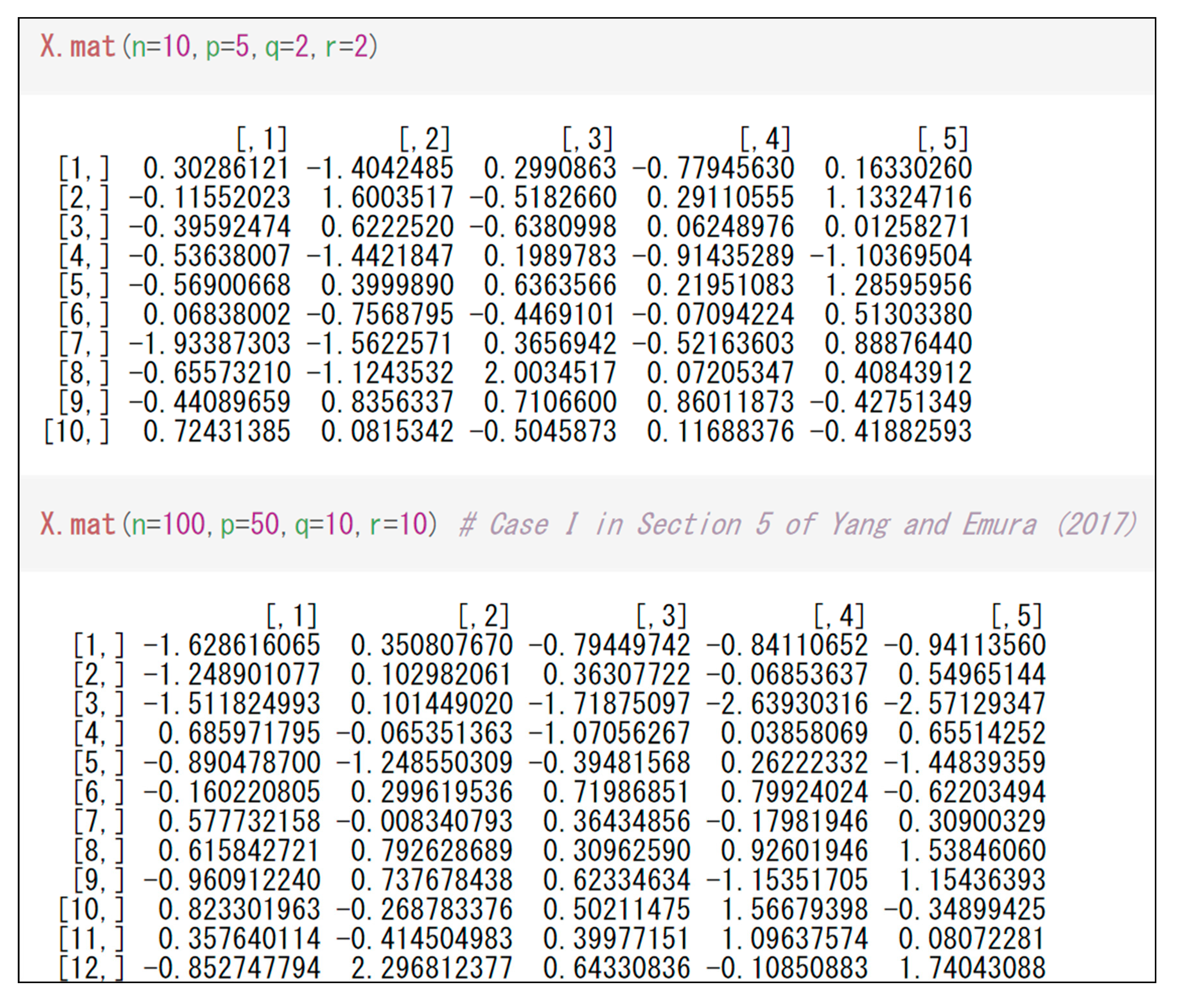
Figure 1 shows an example for generating design matrices using “X.mat(.)”. One can simply input
,
,
, and
into “X.mat(.)” by noting the constraint
.
3.2. Performing regression
The ridge and generalized ridge estimators can be computed by the R function “g.ridge(.)” whose input requires a design matrix and a response vector . Specifically, the command “g.ridge(X, Y, method = "HK", kmax = 500)” can calculate the ridge estimator , where “HK” stands for “Hoerl and Kennard”, and “kmax=500” means the range for estimating . The output of the command includes and . Similarly, the command “g.ridge(X, Y, method = "YE", kmax = 500)” can calculate , where “YE” stands for “Yang and Emura”. The output also displays the plot of against , and its minimizer (the plot of for the generalized ridge).
The R function “g.ridge(.)” can also compute the SE of
, Z-value and
P-value for significance tests (
Section 2.4), and the estimate of the error variance
(
Section 2.3). As in the typical practice of ridge regression, we used the centered responses “Y-mean(Y)” rather than “Y” (will be explained in
Section 3.3). Also, if “X” were not generated by “X.mat”, the scaled design matrix “scale(X)” would be recommended rather than “X” itself.
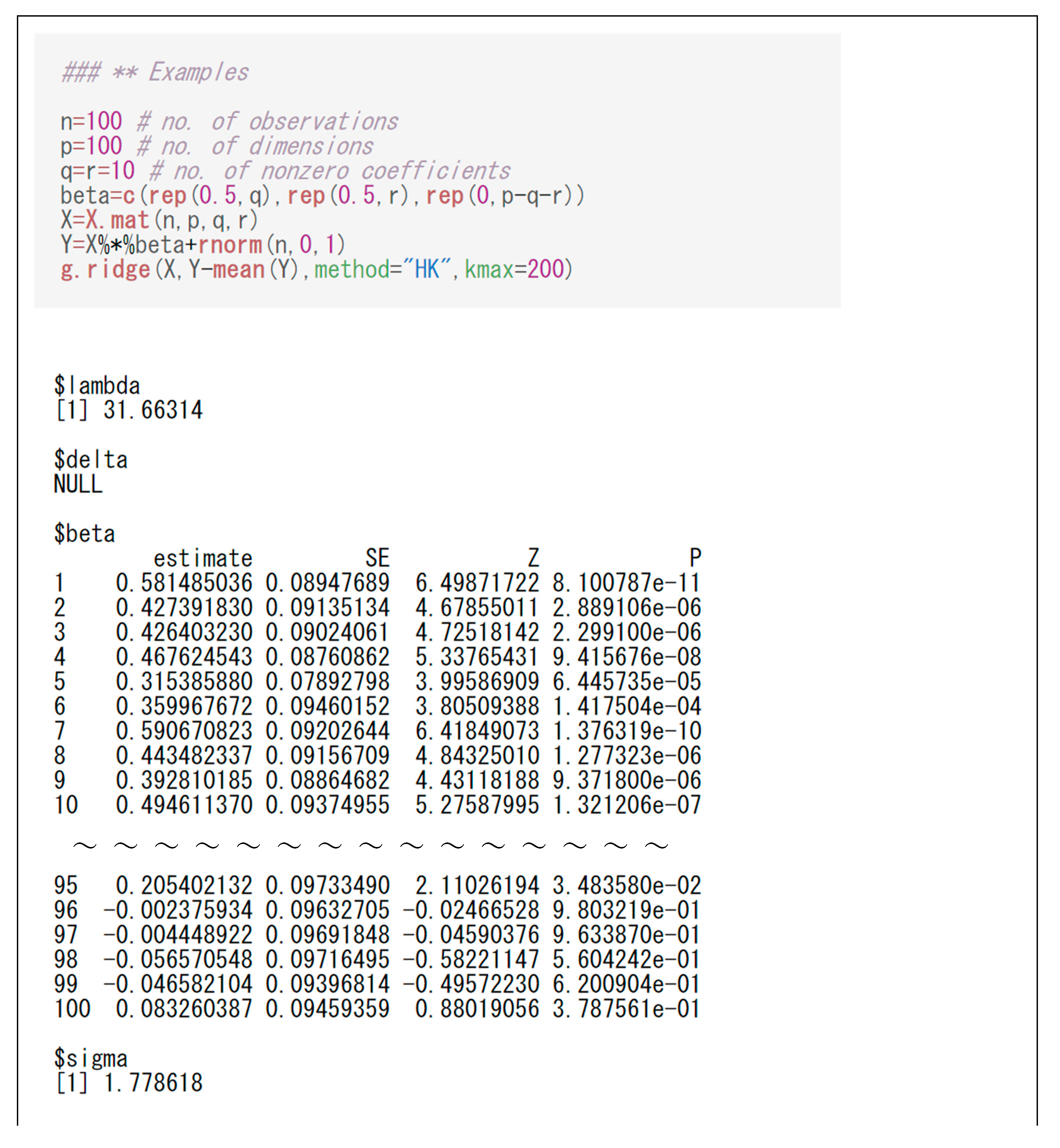
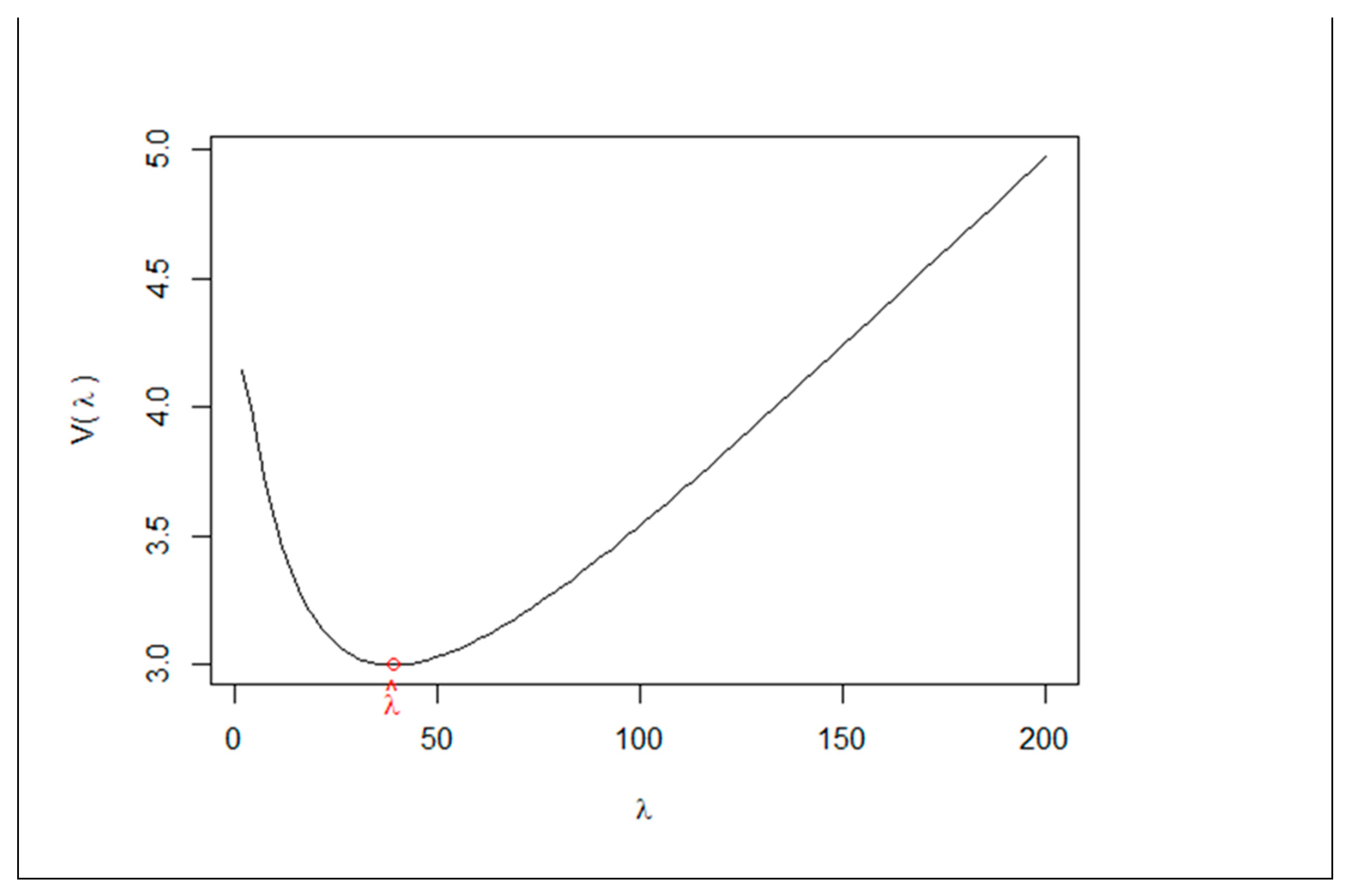
Figure 2 shows the code and output for the ridge estimator. The output shows
,
, SE, Z-value,
P-value, and
. The output also displays the GCV function
against
, showing its minimum at
. In the code, we changed “kmax” from the default value (500) to 200 for a better visualization of the plot. In many cases, users will need to try different values of “kmax” to reach a desirable plot for the GCV function.
The output of the generalized ridge estimator is similar to that of the ridge estimator. Only the difference is an additional parameter estimate shown at “delta$”.
3.3. Technical remarks on centering and standardization
We assume that
is standardized and does not include the intercept term (
Section 2.1). If
is generated by “X.mat”, it is already standardized, and hence there is no need to do the standardization. However, in other cases,
has to be standardized, e.g. by the R command “scale(X)”. By assumption, the design matrix
does not include the intercept term (a column of ones) since one can always use the reduced model
for the intercept model
(
is estimated by
), where
is a vector of ones. This means that the usual unbiased estimator is applied to the intercept.
4. Simulations
We conducted simulation studies to test our R package “g.ridge”. The goals of the simulations are to show: (a) the generalized ridge estimators in our package exhibits superior performance over the ridge estimator in the package “glmnet(.)”, and (b) the sound performance under the normally and non-normally distributed errors (the skew-normal distribution will be considered).
Supplementary Materials include the R code to reproduce the results of the simulation studies.
4.1. Simulation settings
We generated
by “X.mat” with
,
, and
based on Equation (3). Given
, we set
, with
defined by the sparse model:
for four cases: (
I)
; (
II)
; (
III)
,
; (
IV)
,
. Errors
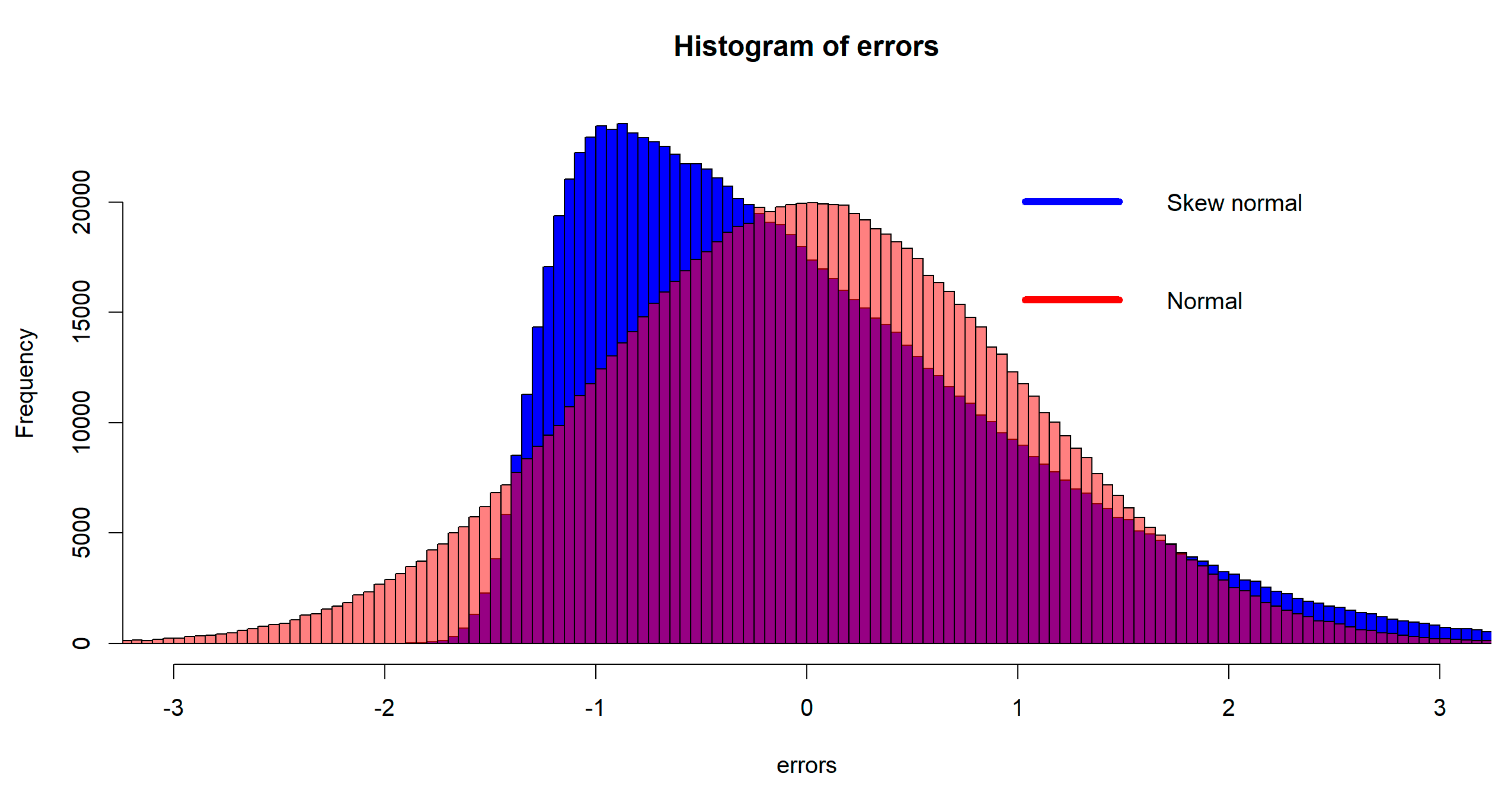
were generated independently from the normal distribution, or the skew-normal distribution (Azzalini 2014); both distributions have mean zero and standard deviation one, and the skew-normal distribution has the slant parameter ten (alpha=10 in the R function “rsn(.)”).
Figure 3 shows the remarkable difference of the two distributions. The skew-normal distribution was not previously examined in the simulation setting of Yang and Emura (2017).
For a given dataset
, we computed
that can be (i) the ridge estimator by “g.ridge(.)”, (ii) the generalized ridge estimator by “g.ridge(.)”, or (iii) the ridge estimator by “glmnet(.)”. Based on 500 replications (on random errors
), the performances of the three proposed estimators were compared by the total mean squared error (TMSE) criterion defined as
where
was performed by the Monte Carlo average over 500 replications.
4.2. Simulation results
Table 1 compares the MSE among the three estimators: (i) the ridge by “g.ridge(.)”, (ii) the generalized ridge by “g.ridge(.)”, and (iii) the ridge by “glmnet(.)”. We see that the generalized ridge estimator is superior to the ridge estimator since the former has smaller TMSE values for all cases. Also, the generalized ridge estimator is superior to the “glmnet(.)” estimator for cases of
while it is not the case for
. This conclusion holds consistently across the four parameter settings (
I)-(
IV) and two error distributions (normal and skew-normal). In conclusion, the generalized ridge estimator in the R proposed package is the most recommended estimator for data with sparse and high-dimensional settings.
5. Data analysis
This section analyzes a real dataset to illustrate the generalized ridge estimator in the proposed package. We retrospectively analyzed a dataset from patients with intracerebral hemorrhage who were hospitalized at Saiseikai Kumamoto Hospital, Kumamoto city, Japan. The study was conducted in accordance with the Declaration of Helsinki, and the protocol was approved by the Ethics Committee of Saiseikai Kumamoto Hospital on March 29, 2023. Saiseikai Kumamoto Hospital is a regional tertiary hospital that serves patients with stroke in southern Japan and provides acute care in a comprehensive stroke care unit.
The outcome variables (
) are the changes of the blood volume (in mL) from the initial value and to the follow-up value, which were measured by the CT scan. Excluding patients with less than 10 mL blood volume at the initial CT scan and other inclusion/exclusion criteria, we arrive at
patients. Regressor variables (
) consist of
continuous measurements, including histological variables (e.g., age), vital signs (e.g., blood pressure, mmHG; respiratory rate, times/minute), and blood measurements (e.g. albumin, g/dL; Gamma-glutamyl transpeptidase (Gamma-GT), IU/L; lactate dehydrogenase, IU/L; Prothrombin time, second; Blood platelet count, 10
-3/μL; C-reactive protein, mg/dL). The responses and regressors are centered and standardized before fitting a linear model as explained in
Section 2.1 and
Section 3.3.
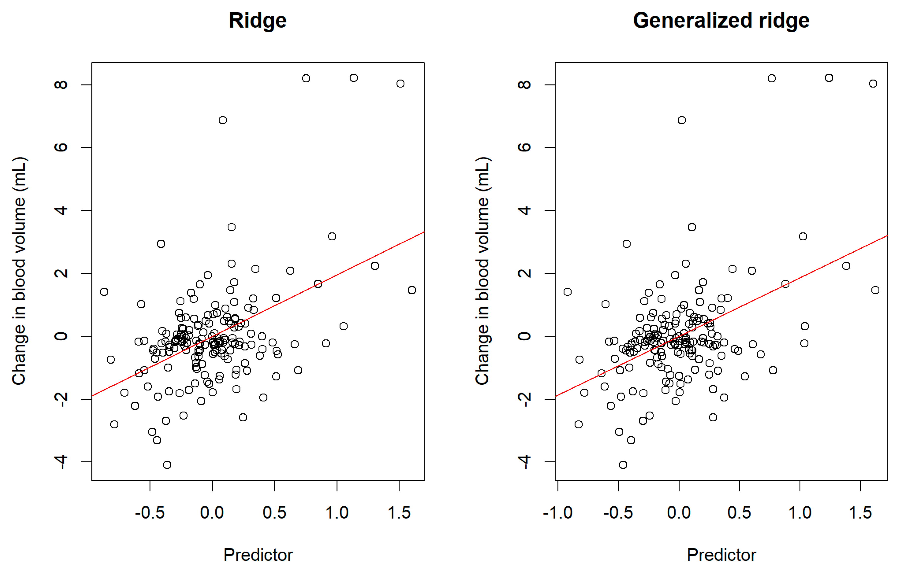
Figure 3 displays scatter plots for the centered responses
against the predictors
based on the ridge estimator and generalized ridge estimator. We observe that the predictors reasonably captured the variability of the changes in the blood volume (response variables). However, the figure also shows that the changes in the blood volumes were not fully explained by the predictors since some residual errors remain.
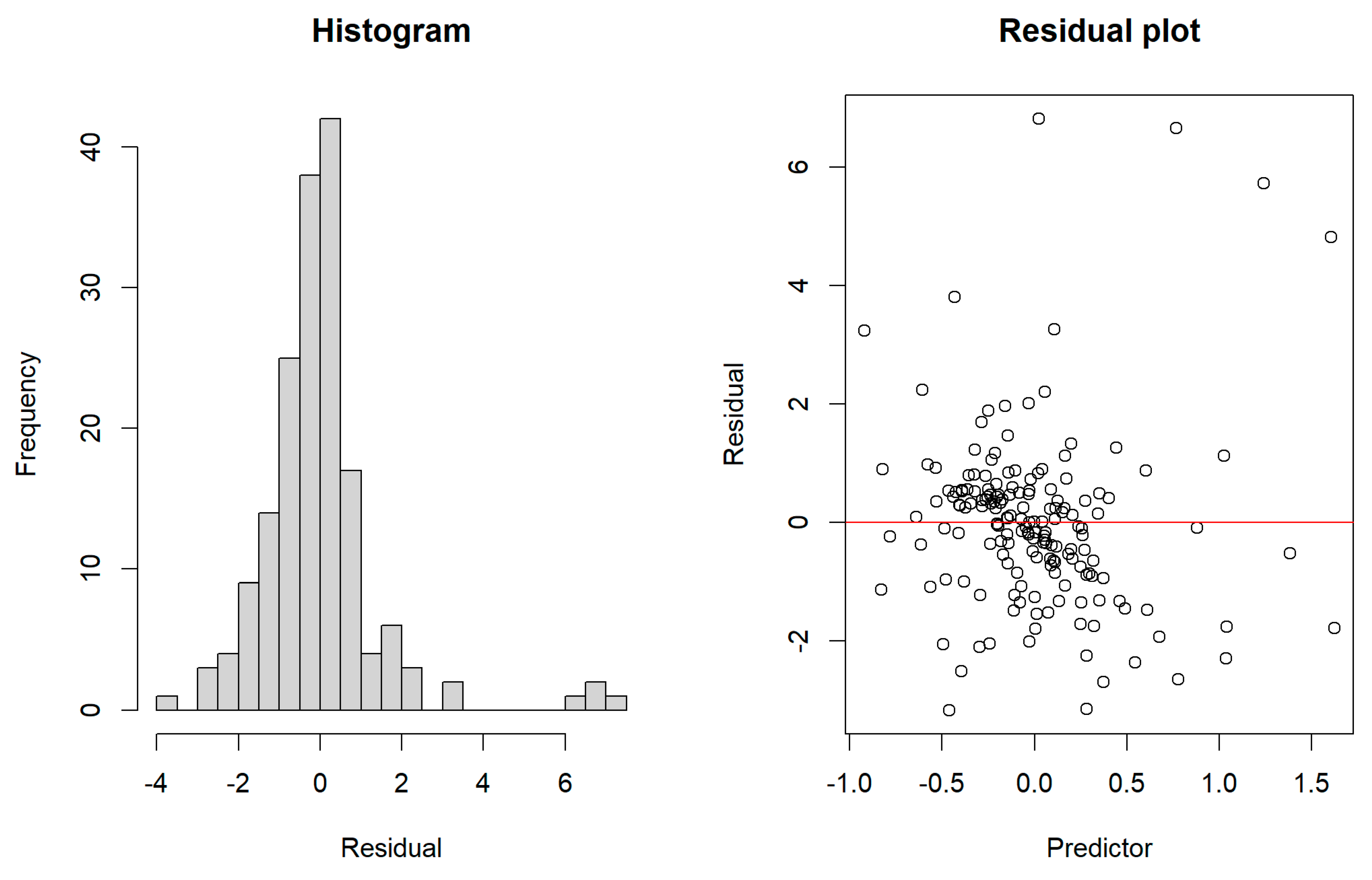
Figure 4 depicts the residuals constructed by the generalized ridge estimator. We observe that the residuals are asymmetric around zero. The asymmetry in the errors does not yield any problem as the proposed ridge estimators was verified for the asymmetric errors (
Section 4).
Table 2 shows the fitted results for estimated regression coefficients sorted by
P-values (only with
P < 0.05). The fitted results are quite similar between the ridge and generalized ridge estimators. The most significant regressor is the lactate dehydrogenase. This variable was previously reported as an important predictor of hematoma expansion (Chu et al. 2019). An interesting difference is found in the number of significant regressors: 6 regressors for the generalized ridge estimator, and 5 regressors for the ridge estimator. That is, the C-reactive protein as a regressor selected solely by the generalized ridge estimator. A study conducted in a large population in China reported that a high C-reactive protein level was an independent risk factor for the severe intracerebral hemorrhage (Wang et al. 2021). The selection of C-reactive protein as a variable associated with increased hematoma volume may reflect the tendency of patients with severe intracerebral hemorrhage to have easier hematoma expansion.
Finally, we compared the performance of the ridge and generalized ridge estimators by means of the residual mean squared error (RMSE) defined as
The RMSE were 2.288 (the ridge estimator) and 2.284 (the generalize ridge estimator). Therefore, the predictor constructed from the generalized ridge estimator had slightly better performance over the one from the ridge estimator.
Therefore, we have demonstrated that the ridge and generalize ridge estimators in the proposed R package provide statistically and biologically sound conclusions on the real data analysis.
6. Conclusion
This paper introduced the new R package “g.ridge” that can perform the ridge and generalized ridge regression methods. We showed that the generalized ridge estimator in the proposed package performs better than the widely used ridge estimator in the “glmnet” package. Furthermore, the ridge and generalized ridge estimators in the proposed package can deal with asymmetric error distributions. With the abundance of sparse and high-dimensional data (Kim et al. 2007; Zhang et al. 2021; Vishwakarma et al. 2021; Bhattacharjee 2022; Bhatnagar et al. 2023; Emura et al. 2023) and asymmetrically distributed data (Abe et al. 2012; Huynh et al. 2021; Yoshiba et al. 2023; Jimichi et al. 2023), the proposed package may provide a reliable statistical tool for statisticians and data scientists.
The generalized ridge estimator considered in this article may be extended to logistic regression, Poisson regression, and Cox regression. Such extensions have not been explored yet. While the extensions might not be technically difficult, well-designed simulation studies and implementations in some software packages will be necessary to fully justify the advantage and usefulness over the usual ridge estimator that is widespread via the “glmnet” package.
Data Availability Statement:
Supplementary Materials include the R code to reproduce the results of the simulation studies. The dataset used in Section 5 is available from the corresponding author on reasonable request.
Institutional Review Board Statement
The study (of
Section 5) was conducted in accordance with the Declaration of Helsinki, and the protocol was approved by the Ethics Committee of Saiseikai Kumamoto Hospital (Approval No. 1156 and March 29, 2023).
Informed Consent Statement
Given the retrospective nature of the study and the use of anonymized patient data in
Section 5, written informed consent was not required. Patients preferred not to be included in this study were given the opportunity to opt out.
Acknowledgements
Emura T is supported financially by the research grant from the JSPS KAKENHI (grant no. 22K11948, and grant no. 20H04147).
Conflicts of Interest
The authors declare that they have no competing interests.
Appendix A. GCV function
The GCV functions are defined as
and
in Equations (1) and (2), respectively. The ridge estimator uses
while the generalized ridge estimator uses
for estimating shrinkage parameters. Therefore, we made an R function “CGV(X,Y,k,W)” to help computing
and
, where “X” is a design matrix, “Y” is a response vector, “k” is actually
(because “lambda” is a long name). Note that “W” can be any square matrix of dimension
to allow for general use. Thus, what we actually compute in “CGV(X,Y,k,W)” is
where
for any symmetric matrix
. However, we normally use
for the ridge or
for the generalized ridge as defined in
Section 2.3.
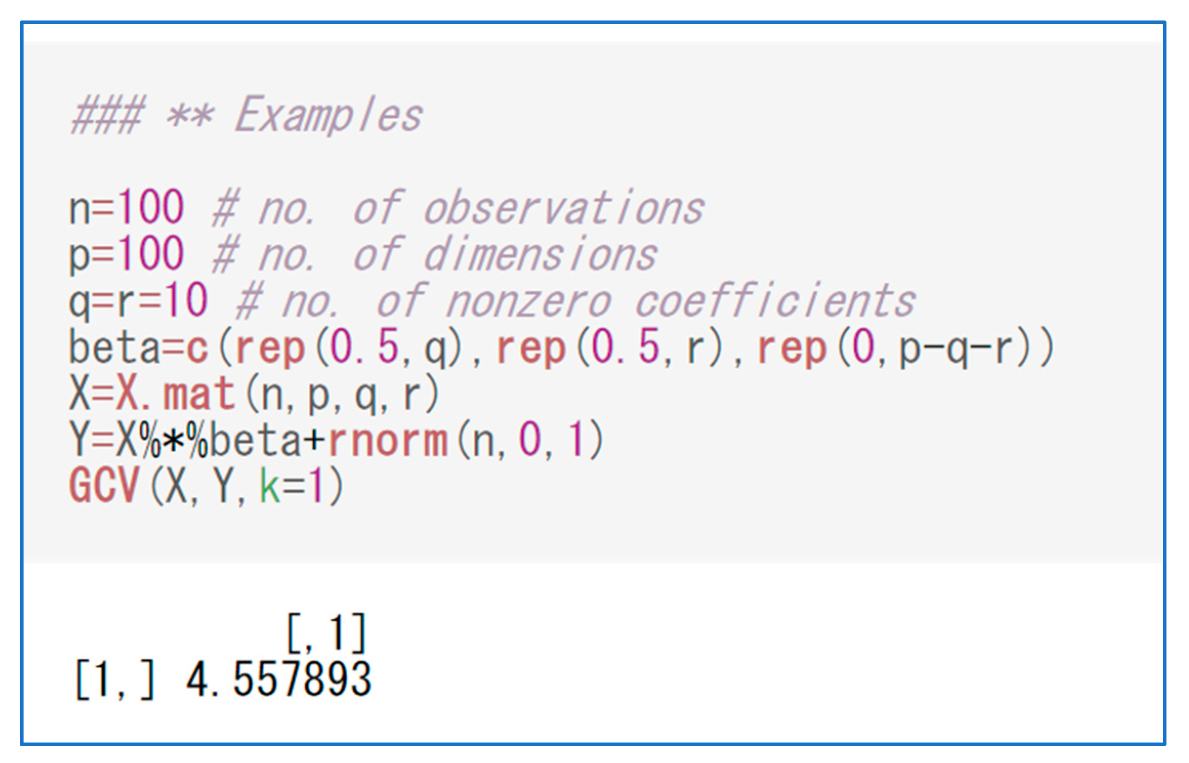
Figure A1 shows the R code for using “CGV(X,Y,k,W)”. The default for “W” is
and therefore “GCV(X,Y,k=1)” can compute
for
, or equivalently,
for
.
Figure A1.
An example for using “CGV(X,Y,k,W)”.
Figure A1.
An example for using “CGV(X,Y,k,W)”.
References
- Abe, T.; Shimizu, K.; Kuuluvainen, T.; Aakala, T. Sine-skewed axial distributions with an application for fallen tree data. Environ. Ecol. Stat. 2012, 19, 295–307. [Google Scholar] [CrossRef]
- Allen, D.M. The relationship between variable selection and data augmentation and a method for prediction. Technometrics 1974, 16, 125–127. [Google Scholar] [CrossRef]
- Arashi, M.; Roozbeh, M.; Hamzah, N.A.; Gasparini, M. Ridge regression and its applications in genetic studies. PLOS ONE 2021, 16, e0245376. [Google Scholar] [CrossRef]
- Assaf, A.G.; Tsionas, M.; Tasiopoulos, A. Diagnosing and correcting the effects of multicollinearity: Bayesian implications of ridge regression. Tour. Manag. 2019, 71, 1–8. [Google Scholar] [CrossRef]
- Azzalini, A.; Capitanio, A. The Skew-Normal and Related Families; IMS Monographs series; Cambridge University Press (CUP): Cambridge, UK, 2014. [Google Scholar]
- Binder, H.; Allignol, A.; Schumacher, M.; Beyersmann, J. Boosting for high-dimensional time-to-event data with competing risks. Bioinformatics 2009, 25, 890–896. [Google Scholar] [CrossRef]
- Bhattacharjee, A. Big Data Analytics in Oncology with R; CRC Press: Boca Raton, FL, USA, 2022. [Google Scholar]
- Bhatnagar, S.R.; Lu, T.; Lovato, A.; Olds, D.L.; Kobor, M.S.; Meaney, M.J.; O'Donnell, K.; Yang, A.Y.; Greenwood, C.M. A sparse additive model for high-dimensional interactions with an exposure variable. Comput. Stat. Data Anal. 2023, 179. [Google Scholar] [CrossRef]
- Chen, A.-C.; Emura, T. A modified Liu-type estimator with an intercept term under mixture experiments. Commun. Stat. - Theory Methods 2017, 46, 6645–6667. [Google Scholar] [CrossRef]
- Chu, H.; Huang, C.; Dong, J.; Yang, X.; Xiang, J.; Dong, Q.; Tang, Y. Lactate Dehydrogenase Predicts Early Hematoma Expansion and Poor Outcomes in Intracerebral Hemorrhage Patients. Transl. Stroke Res. 2019, 10, 620–629. [Google Scholar] [CrossRef]
- Cule, E.; De Iorio, M. Ridge regression in prediction problems: automatic choice of the ridge parameter. Genetic Epidemiology 2013, 37, 704–714. [Google Scholar] [CrossRef]
- Cule, E.; Vineis, P.; De Iorio, M. Significance testing in ridge regression for genetic data. BMC Bioinform. 2011, 12, 372–372. [Google Scholar] [CrossRef]
- Emura, T.; Chen, Y.-H.; Chen, H.-Y. Survival Prediction Based on Compound Covariate under Cox Proportional Hazard Models. PLOS ONE 2012, 7, e47627. [Google Scholar] [CrossRef]
- Emura, T.; Chen, Y.-H. Gene selection for survival data under dependent censoring: A copula-based approach. Stat. Methods Med Res. 2016, 25, 2840–2857. [Google Scholar] [CrossRef]
- Emura, T.; Hsu, W.-C.; Chou, W.-C. A survival tree based on stabilized score tests for high-dimensional covariates. J. Appl. Stat. 2023, 50, 264–290. [Google Scholar] [CrossRef]
- Friedrich, S.; Groll, A.; Ickstadt, K.; Kneib, T.; Pauly, M.; Rahnenführer, J.; Friede, T. Regularization approaches in clinical biostatistics: A review of methods and their applications. Stat. Methods Med Res. 2023, 32, 425–440. [Google Scholar] [CrossRef]
- Gao, S.; Zhu, G.; Bialkowski, A.; Zhou, X. Stroke Localization Using Multiple Ridge Regression Predictors Based on Electromagnetic Signals. Mathematics 2023, 11, 464. [Google Scholar] [CrossRef]
- Golub, G.H. , Heath, M.; Wahba, G. Generalized cross-validation as a method for choosing a good ridge parameter. Technometrics 1979, 21, 215–223. [Google Scholar] [CrossRef]
- Hastie, T.; Tibshirani, R.; Friedman, J. The Elements of Statistical Learning; Springer: New York, NY, USA, 2009. [Google Scholar]
- Hernandez, J.; Lobos, G.A.; Matus, I.; Del Pozo, A.; Silva, P.; Galleguillos, M. Using Ridge Regression Models to Estimate Grain Yield from Field Spectral Data in Bread Wheat (Triticum aestivum L.) Grown under Three Water Regimes. Remote Sens. 2015, 7, 2109–2126. [Google Scholar] [CrossRef]
- Hoerl, A.E.; Kennard, R.W. Ridge regression: Biased estimation for nonorthogonal problems. Technometrics 1970, 12, 55–67. [Google Scholar] [CrossRef]
- Huynh, U.; Pal, N.; Nguyen, M. Regression model under skew-normal error with applications in predicting groundwater arsenic level in the Mekong Delta Region. Environ. Ecol. Stat. 2021, 28, 323–353. [Google Scholar] [CrossRef]
- Jimichi, M.; Kawasaki, Y.; Miyamoto, D.; Saka, C.; Nagata, S. Statistical Modeling of Financial Data with Skew-Symmetric Error Distributions. Symmetry 2023, 15, 1772. [Google Scholar] [CrossRef]
- Kibria, B.M.G.; Banik, S. Some Ridge Regression Estimators and Their Performances. J. Mod. Appl. Stat. Methods 2016, 15, 206–238. [Google Scholar] [CrossRef]
- Kim, S.Y.; Lee, J.W. Ensemble clustering method based on the resampling similarity measure for gene expression data. Stat. Methods Med Res. 2007, 16, 539–564. [Google Scholar] [CrossRef] [PubMed]
- Loesgen, K.H. A generalization and Bayesian interpretation of ridge-type estimators with good prior means. Stat. Pap. 1990, 31, 147–154. [Google Scholar] [CrossRef]
- Montgomery, D.C.; Peck, E.A.; Vining, G.G. Introduction to Linear Regression Analysis; John Wiley & Sons: Hoboken, NJ, USA, 2021. [Google Scholar]
- Michimae, H.; Emura, T. Bayesian ridge estimators based on copula-based joint prior distributions for regression coefficients. Comput. Stat. 2022, 37, 2741–2769. [Google Scholar] [CrossRef]
- Norouzirad, M.; Arashi, M. Preliminary test and Stein-type shrinkage ridge estimators in robust regression. Stat. Pap. 2019, 60, 1849–1882. [Google Scholar] [CrossRef]
- Saleh, E.A.M.; Kibria, G.B.M. Performance of some new preliminary test ridge regression estimators and their properties. Communications in Statistics-Theory and Methods 1993, 22, 2747–2764. [Google Scholar] [CrossRef]
- Saleh, A.M.E.; Arashi, M.; Kibria, B.G. Theory of Ridge Regression Estimation with Applications; John Wiley & Sons: Hoboken, NJ, USA, 2019. [Google Scholar]
- Shih, J.-H.; Lin, T.-Y.; Jimichi, M.; Emura, T. Robust ridge M-estimators with pretest and Stein-rule shrinkage for an intercept term. Jpn. J. Stat. Data Sci. 2021, 4, 107–150. [Google Scholar] [CrossRef]
- Shih, J.H. , Konno, Y., Chang, Y.T.; Emura, T. A class of general pretest estimators for the univariate normal mean. Communications in Statistics-Theory and Methods 2023, 52, 2538–2561. [Google Scholar] [CrossRef]
- Taketomi, N.; Chang, Y.-T.; Konno, Y.; Mori, M.; Emura, T. Confidence interval for normal means in meta-analysis based on a pretest estimator. Jpn. J. Stat. Data Sci. 2023, 1–32. [Google Scholar] [CrossRef]
- Vishwakarma, G.K.; Thomas, A.; Bhattacharjee, A. A weight function method for selection of proteins to predict an outcome using protein expression data. J. Comput. Appl. Math. 2021, 391, 113465. [Google Scholar] [CrossRef]
- Wang, D.; Wang, J.; Li, Z.; Gu, H.; Yang, K.; Zhao, X.; Wang, Y. C-Reaction Protein and the Severity of Intracerebral Hemorrhage: A Study from Chinese Stroke Center Alliance. Neurol. Res. 2021, 44, 285–290. [Google Scholar] [CrossRef] [PubMed]
- Whittaker, J.C.; Thompson, R.; Denham, M.C. Marker-assisted selection using ridge regression. Genet. Res. 2000, 75, 249–252. [Google Scholar] [CrossRef] [PubMed]
- Wong, K.Y.; Chiu, S.N. An iterative approach to minimize the mean squared error in ridge regression. Comput. Stat. 2015, 30, 625–639. [Google Scholar] [CrossRef]
- Yang, S.-P.; Emura, T. A Bayesian approach with generalized ridge estimation for high-dimensional regression and testing. Commun. Stat. - Simul. Comput. 2017, 46, 6083–6105. [Google Scholar] [CrossRef]
- Yoshiba, T.; Koike, T.; Kato, S. On a Measure of Tail Asymmetry for the Bivariate Skew-Normal Copula. Symmetry 2023, 15, 1410. [Google Scholar] [CrossRef]
- Yüzbaşı, B.; Arashi, M.; Ahmed, S.E. Shrinkage Estimation Strategies in Generalised Ridge Regression Models: Low/High-Dimension Regime. Int. Stat. Rev. 2020, 88, 229–251. [Google Scholar] [CrossRef]
- Zhang, Q.; Ma, S.; Huang, Y. Promote sign consistency in the joint estimation of precision matrices. Comput. Stat. Data Anal. 2021, 159, 107210. [Google Scholar] [CrossRef]
|
Disclaimer/Publisher’s Note: The statements, opinions and data contained in all publications are solely those of the individual author(s) and contributor(s) and not of MDPI and/or the editor(s). MDPI and/or the editor(s) disclaim responsibility for any injury to people or property resulting from any ideas, methods, instructions or products referred to in the content. |
© 2024 by the authors. Licensee MDPI, Basel, Switzerland. This article is an open access article distributed under the terms and conditions of the Creative Commons Attribution (CC BY) license (http://creativecommons.org/licenses/by/4.0/).

