1. Introduction
Smart homes have gained significant popularity since the late 1990s, offering occupants comfort and energy-efficient solutions [
1]. These technologies allow homes to learn from their environment and adjust settings to meet occupants’ preferences while minimizing operational costs. The adoption of smart home technologies not only enhances occupant comfort and energy efficiency but also supports independent living for the elderly, people with dementia, and individuals with intellectual disabilities. Furthermore, smart homes play a crucial role in patient homecare and monitoring [
2,
3].
The driving forces behind smart homes are communication technology, especially the Internet of Things (IoT), and intelligent algorithms that provide homes with the necessary intelligence. This study focuses on intelligent algorithms that enable smart homes to maximize occupant comfort while minimizing energy consumption. These objectives are interconnected yet contradictory. For instance, thermal comfort is essential for overall comfort, with air conditioning being used in tropical countries to lower indoor temperatures, while heating systems are crucial in temperate climates during winter. However, the usage of heating, ventilation, and air-conditioning (HVAC) systems contributes significantly to energy consumption in buildings [
4,
5].
To address these contradictory challenges, optimizing the settings of electrical appliances can be employed. Occupant comfort is influenced by various factors, including temperature, indoor air quality (IAQ), and illumination. This study focuses on maximizing the comfort index by considering these parameters, as they have a significant impact on the mental and physical health of occupants [
6], ultimately affecting their overall comfort. Maintaining optimal indoor temperature is vital, as extreme temperatures can have adverse effects on occupants’ health. Similarly, ensuring healthy IAQ is essential to prevent sick building syndrome and maintain occupants’ productivity [
7]. Additionally, appropriate indoor illumination plays a crucial role in regulating the human circadian clock, positively impacting occupants’ quality of life and well-being [
8].
Controlling these parameters is possible through the use of air conditioning systems, air ventilators, and lighting. However, these systems consume substantial amounts of energy. Hence, this study also aims to minimize energy usage by these appliances, achieving energy efficiency in smart homes [
9]. In addition to these efforts, the integration of digital twin technology provides a comprehensive approach to optimize user comfort and energy efficiency. A digital twin [
10,
11] consists of multiple modules, including a physical layout, computer models, data analysis, and communication platforms. These components are coordinated and operate in unison to study, oversee, and enhance the overall performance of the system. Implementing a digital twin necessitates the creation of innovative methods, processes, and software to enable efficient communication and collaboration among the different modules. This paper introduces a detailed model that combines different methods to make sure smart homes are as comfortable as possible while using energy efficiently. The model has three main parts: smoothing, optimization, and control. The smoothing part makes sure the data we use to predict how much energy we’ll use is clear and accurate. The optimization part uses machine learning, a type of artificial intelligence, to change settings in the home to keep it comfortable while using less energy. The control part makes sure that energy is delivered in the most efficient way to make people in the home comfortable.
After comparing our model to others already available, we have determined that our model is more superior. We also found that using flexible control systems and improved methods to optimize energy use are really important in making homes both comfortable and energy efficient.
In the realm of smart home technology [
12], the integration of "digital twin" and fuzzy logic controller [
13] is becoming increasingly transformative. At its core, a digital twin offers a dynamic digital blueprint of a home’s physical environment, driven by sensor-collected data on key parameters like temperature, air quality, and lighting. This real-time data serves as the foundation upon which the fuzzy logic controller operates [
14]. Unlike traditional binary logic systems, a fuzzy logic controller excels in making decisions based on imprecise or "fuzzy" input values, thereby enabling more nuanced adjustments. For instance, if the digital twin detects a slightly elevated room temperature combined with increased humidity, the fuzzy logic controller might determine an optimal thermostat setting that accounts for both comfort and energy efficiency. Similarly, in assessing air quality, the controller could make incremental ventilation adjustments, ensuring a balanced and healthy atmosphere. Moreover, when analyzing lighting conditions, it doesn’t just switch lights on or off but might modulate light intensity based on the time of day, user preferences, and available natural light. In combining the predictive power of a digital twin with the nuanced decision-making of a fuzzy logic controller, smart homes are better equipped to achieve a seamless blend of user comfort and energy conservation.
In conclusion, this study aims to leverage digital twin technology and advanced algorithms to achieve efficient energy consumption optimization and enhanced user comfort in smart homes. By integrating intelligent algorithms, optimization modules, and digital twin capabilities, this research contributes to the advancement of smart home technologies, benefiting occupants, energy efficiency, and overall quality of life. In our work, we have also introduced a model that utilizes smoothing algorithms, optimization algorithms, machine learning algorithms, and control algorithms.
The primary goals of the proposed work are as follows:
To enhance the comfort level of users in smart homes
To reduce energy consumption in smart homes with improved comfort
The Idea of Digital Twin
To identify optimal user-defined parameters through the utilization of an advanced machine learning algorithm
The organization of the paper will proceed as follows:
Section 2 provides a detailed presentation of the proposed methodology,
Section 3 covers the implementation, results, and comparative analysis, and finally,
Section 4 concludes the paper.
2. Related Work
Many people and companies are working hard to find ways to use less energy while still keeping homes comfortable. Saving energy is important because it costs a lot, and we want to take care of our planet. There is a need for tools and methods that can help us use energy wisely without making life uncomfortable. One exciting development is the use of advanced technologies and simulations. These tools can be used to test out different ways to save energy and keep comfort levels high. This could be the key to solving the challenge of using less energy while keeping our homes comfortable. These advanced technologies have demonstrated considerable capabilities in smart home and other sectors.
In [
15], the evolutionary accretive comfort algorithm (EACA) is introduced. EACA, based on a genetic algorithm (GA), aims to maximize user comfort while adhering to predefined cost constraints. Comfort optimization relies on the usage of appliances, prioritized according to consumer preferences. The proposed EACA can achieve optimal comfort within specified cost limits. It’s important to note that higher comfort levels can be attained by allocating more resources, thus increasing the cost.
In a related study, [
16] employs the non-dominated sorting genetic algorithm II (NSGA-II) for optimizing both thermal comfort and energy usage. NSGA-II seeks solutions forming a Pareto front, optimizing both objectives simultaneously. Thermal comfort is evaluated based on Fanger’s predicted mean vote (PMV) and responses obtained from surveys, while energy consumption is quantified using annual gas and electricity consumption data. This technique effectively maintains thermal comfort levels while reducing overall energy consumption. A similar approach is found in [
17], where NSGA-II is utilized to minimize energy usage while ensuring thermal comfort. This is achieved by optimizing factors such as humidity, airspeed, temperature, and the percentage of dissatisfied individuals in a given venue.
In [
18], a Genetic Algorithm (GA) is employed to determine optimal values for temperature, Indoor Air Quality (IAQ), and illumination that contribute to user comfort. These optimal values, along with environmental data, are then input into a fuzzy controller to minimize the required power consumption. In contrast, [
19] treats user comfort maximization and energy usage minimization as a single objective problem by using a weighted penalty function. The parameters considered for determining both comfort and energy usage include indoor temperature, illumination, and IAQ. The results indicate that GA is more effective at reducing energy consumption compared to Particle Swarm Optimization (PSO), while PSO excels in maximizing the comfort index.
Meanwhile, in [
20,
21], GA is hybridized with the Firefly Algorithm (FA) to optimize temperature, IAQ, and illumination. This combination of algorithms addresses the issue of imbalanced exploration and exploitation in FA, resulting in improved performance compared to the original FA and GA when solving the same problem. Following optimization, the parameters are input into a fuzzy controller to minimize energy consumption. Several other works, such as [
22], utilize similar approaches to [
18,
20,
21] but employ different swarm intelligence algorithms. For instance, [
23] employs the Artificial Bees Algorithm (ABC) and uses ABC with a knowledge base, while [
24] utilizes the original Bat Algorithm (BA). These algorithms are applied to optimize parameters related to user comfort and energy efficiency in a similar manner as described in the aforementioned references.
In [
25], a chaotic Bat Algorithm (BA) is employed for fine-tuning the parameters of residential HVAC controllers. This optimization aims to achieve the dual objectives of optimizing energy usage and enhancing thermal comfort. Additionally, the chaotic BA is applied to the task of tuning the coal feed rate in an industrial precalciner temperature control loop, with the goal of optimizing energy usage in this industrial context. [
26] focuses on the optimization of illumination comfort levels and power usage for lighting systems. The authors introduce a novel illumination comfort metric called the Illuminance Uniformity Deviation Index (IUDI). They utilize a multi-objective Particle Swarm Optimization (PSO) approach to simultaneously optimize both illumination comfort and power usage. The IUDI considers factors such as illuminance uniformity and daylight contribution factor for indoor illumination when calculating the comfort level, contributing to a more comprehensive optimization of lighting conditions.
In [
27], an Internet of Things (IoT) system designed for personalized comfort management is introduced. In their research, they focus on representing comfort using ontologies, drawing from classes derived from the DogOnt ontology [
28] and the Semantic Sensor Network (SSN) ontology [
29]. A similar approach is employed in [
30], where an indoor environmental comfort system utilizes a domain ontology to formalize concepts related to sensors and actuators. While this work does not explicitly model comfort metrics, it does involve the acquisition of contextual data, which is subsequently processed using semantic rules. The topic of air quality is explored in [
31], which proposes an ontology that formalizes certain aspects of the ISO 7730:2005 standard. BOnSAI [
32], an ontology developed to facilitate the integration of Ambient Intelligence (AmI) in smart buildings, also includes some comfort-related concepts. Although primarily dedicated to describing device functionalities, services, and hardware, BOnSAI encompasses contextual elements representing comfort and users. Similarly, ThinkHome [
33] presents a semantic model aimed at encompassing the entire Smart Home (SH) ecosystem, thus incorporating concepts related to comfort.
In [
34], a semantic model is introduced for representing thermal comfort within a semantic framework designed for automated modeling of cyber-physical systems. In [
35], the authors address the modeling of indoor comfort metrics by reusing reference models, allowing for the customization of comfort in cruise cabins. In this context, the ontology serves as a foundational framework for an IoT system aimed at monitoring and enhancing the cruise experience.
Many people and companies are working hard to find ways to use less energy while still keeping homes comfortable. Saving energy is important because it costs a lot, and we want to take care of our planet. There is a need for tools and methods that can help us use energy wisely without making life uncomfortable. One exciting development is the use of something called a Digital Twin (DT). It’s like a virtual copy of a home that can be used to test out different ways to save energy and keep comfort levels high. This could be the key to solving the challenge of using less energy while keeping our homes comfortable.
The DT has demonstrated considerable capabilities in smart home and other sectors. This section provides a review of relevant studies, concisely outlined in Table I, with detailed discussions in the subsequent subsections.
3. Problem Formulation
Consider the current sensor measurements for temperature, illumination, and air quality represented as
. Occupants define their comfort range for each parameter. These ranges are specified by user set points:
where:
The assumption is that the maximum value in the range signifies the most preferred setting, while the minimum represents the least acceptable value. Ideally, if energy costs were negligible, users would prefer settings at their maximum values. However, due to high energy costs, a balance between energy consumption and user comfort becomes necessary. We define the range length for each parameter as , , and .
Assume the energy consumption per unit change in each parameter is given by for temperature, illumination, and air quality, respectively. In an ideal situation without energy constraints, parameters would be set as per user preference. However, practical scenarios require a compromise between energy efficiency and comfort. Table 1 summarizes the notations used in this formulation. Note that this formulation applies to heating scenarios (winter). For cooling scenarios (summer), the equations will be slightly modified.
Optimal parameter values are denoted as
, which can lie within the user-specified range. The total energy required for maintaining these optimal settings is given by:
We can also determine the potential minimum and maximum energy consumption:
Our goal is to maximize user comfort and energy savings. This can be abstractly represented as:
where
is the gain in user comfort,
is the gain in energy savings, and
and
are the respective weights, satisfying:
User comfort gain is formulated as:
where
defines the preference for each parameter. The gain in energy savings is inversely proportional to energy consumption:
Using these formulations, our optimization function becomes:
Constraints are defined as:
4. Proposed Methodology
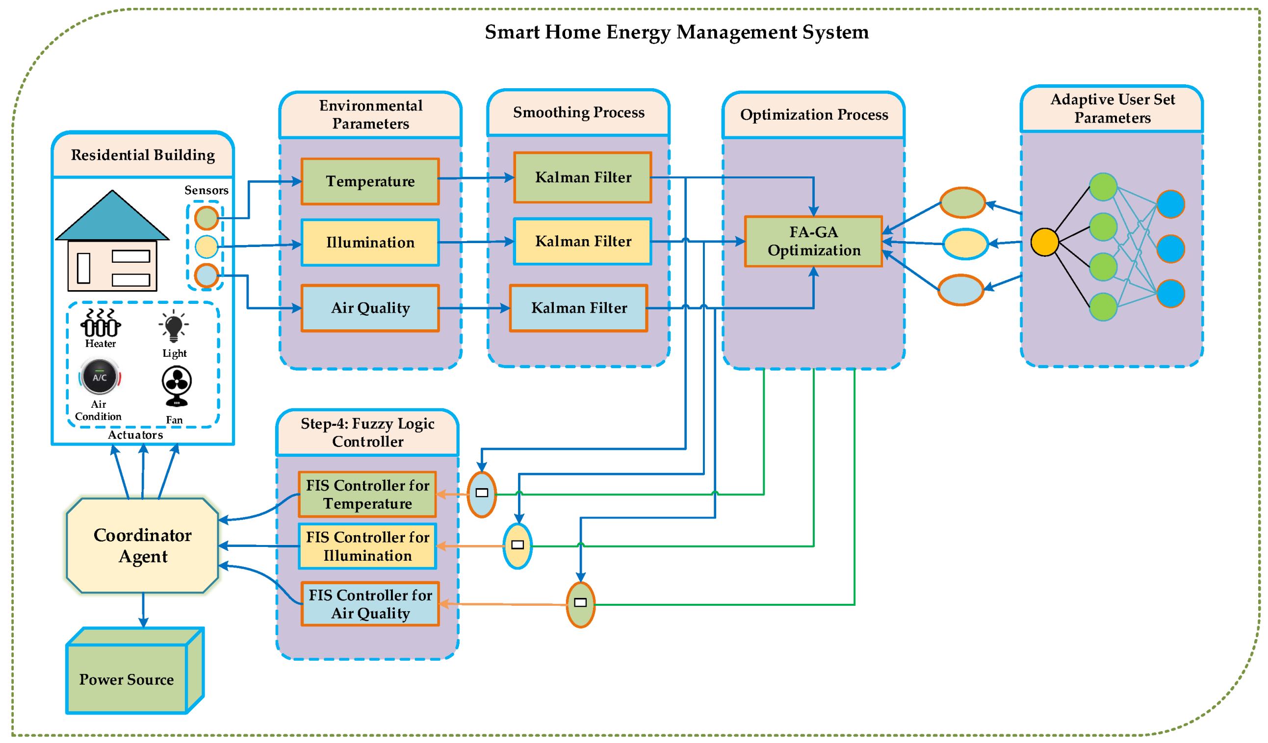
The proposed model comprises three main modules: the smoothing module, optimization module, and control module. The smoothing module utilizes various algorithms (e.g., Kalman filter [
36], alpha-beta filter [
37,
38,
39]) to eliminate sensor data noise and handle missing values. In the optimization module, different algorithms such as the firefly algorithm, and genetic algorithm, are employed. This module also incorporates the comfort index formula, which is fine-tuned using machine learning algorithms to adapt to user-defined factors, thereby enhancing system dynamism and autonomy. The control module applies several control algorithms (e.g., Mamdani FIS [
13], Sugeno FIS, PID) to provide the desired energy to actuators through the agent.
Figure 1 illustrates a conceptual structure diagram of the proposed model.
The comfort index is inversely related to the error change, which is determined by the environmental parameters and machine learning set parameters. Power consumption is affected by the difference in error, and a smaller error difference leads to a higher comfort index. Consequently, the problem becomes a multifunctional optimization challenge that aims to minimize power consumption while maximizing the comfort index.
After calculating the comfort index, the next step involves controlling the state of other actuators. Fuzzy controllers are employed to determine the error between environmental boundaries and optimized parameters. The regulator’s output tells us how much power is needed to control things in the house like cooling/heating, lighting, and ventilation. This power is then given to those systems based on what the regulator says is needed. The fuzzy controller uses the best values from special methods we use to get the most efficient results, and it also considers the limits of the environment, like temperature, lighting, and air quality, to decide its output. What the fuzzy controller decides depends on the difference between the actual conditions in the environment and the best values we got from our special methods for things like temperature, lighting, and air quality.
The optimization algorithms aim to minimize the difference between the values set by smart home users and the predicted values. This difference would be significant without applying optimization algorithms, requiring higher output values and increased power consumption. By employing optimization techniques, the difference is reduced, leading to more efficient energy usage. In the proposed work, we will utilize the learning to optimization algorithms module, which is further divided into the learning and optimization modules. The learning module employs artificial neural networks (ANN) [
10] to make the user-set parameters dynamic within the optimization algorithms module. The primary goal of the optimization technique is to minimize the gap between the user’s preferred parameters and the parameters derived from the surrounding environment.
The optimization module aims to increase the comfort index and reduce power usage. One way to decrease power consumption is by minimizing the gap between user preferences and environmental parameters. Achieving closer alignment between these parameters ultimately leads to lower power consumption. The learning-to-optimization module provides the optimized parameters, while the learning-to-fuzzy logic module takes these optimized parameter values as inputs and determines the energy required for the actuators. The coordinator’s agent receives the output from the fuzzy controller as inputs and adjusts the actuators accordingly.
4.1. Kalman Filter Algorithm
The Kalman Filter is known for its effectiveness and ability to work well without needing a lot of historical data. It uses information from the last known state to make smart predictions about a system’s current state. One key part of this model is the Kalman gain (K), which helps balance the system’s own predictions with data from sensors.
Noise from the environment is a common problem that can make sensor readings less accurate. In this study, we’re looking at a temperature sensor, denoted as that’s affected by this kind of noise. The Kalman filter uses a special model to make an educated guess about the system’s state (like an estimated temperature). It then compares this guess with the actual data from the sensor to come up with a more accurate temperature reading for the next moment in time .
An initial step involves the calculation of the temperature predicted,
, derived from the predecessor value estimated through:
Here, represents the predicted temperature internally, while X and Y are the state transition and control matrices, respectively. is the prior temperature reading, and is the control vector.
Uncertainty in this internal prediction is quantified by a covariance factor, updated as:
Where X and are the state transition matrix and its transpose, is the preceding covariance value, and Q denotes the estimated process error.
Subsequent to this, the Kalman gain,
K, undergoes an update via:
Here, the observation matrix and its transpose are signified by
H and
, with
R denoting the estimated error measurement.
Assuming the sensor’s reading temperature at time
t is
, the refined estimated temperature is obtained through:
Conclusively, the covariance is updated for subsequent iterations via:
This explanation highlights how well the Kalman Filter can reduce noise, ensuring accurate measurements. This is especially important in settings where sensor readings can be easily distorted or affected by surrounding conditions.
4.2. Optimization Framework
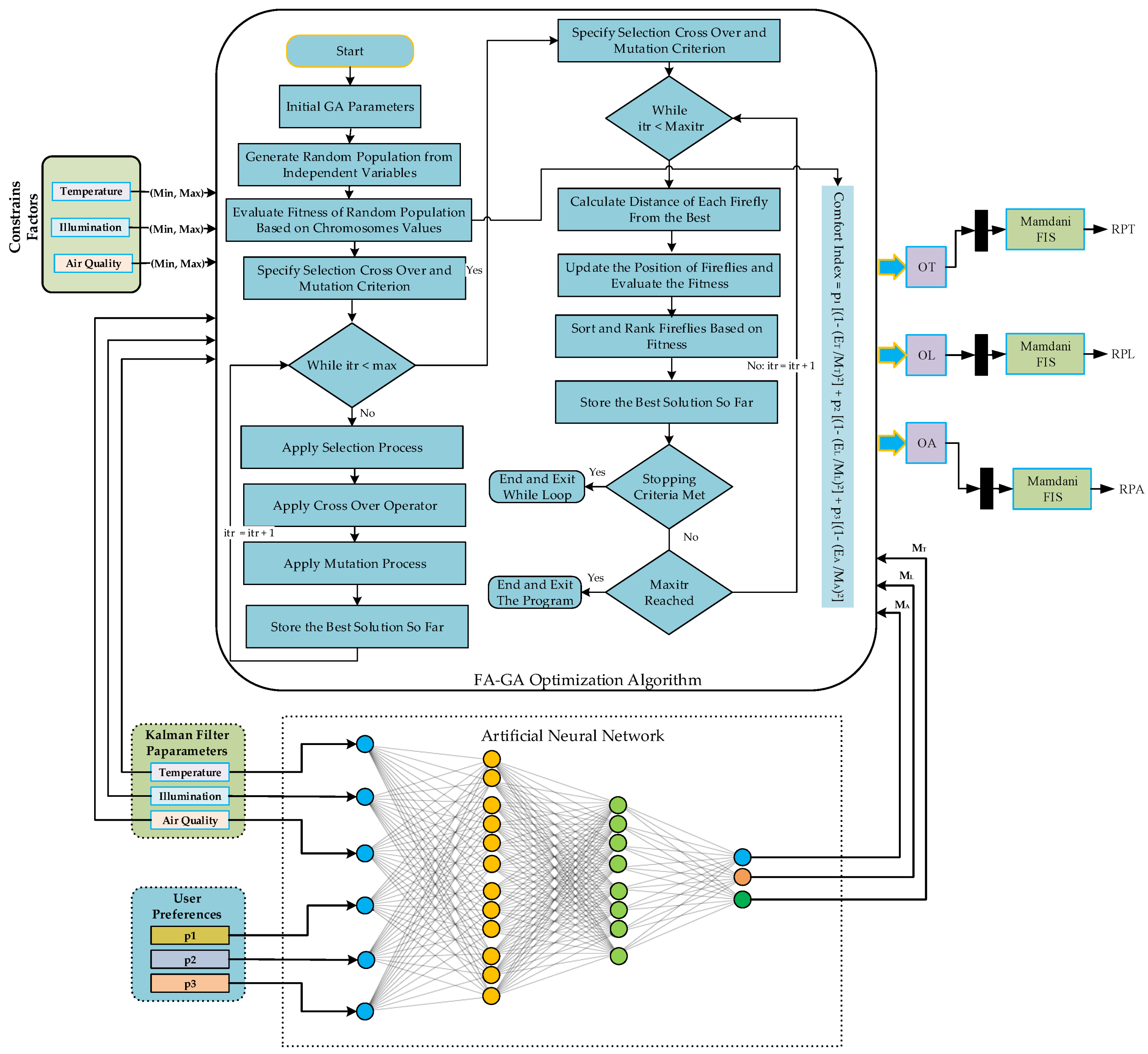
The optimization framework comprises two main modules: the FA-GA module and the artificial neural network (ANN) segment. Initially, the ANN is trained utilizing historical user data. It accepts smooth parameters and outputs user-defined settings. The FA-GA module then evaluates the discrepancy between the ANN’s output and these smooth parameters. These derived parameters play a pivotal role in the comfort index formula within the FA-GA algorithm, as depicted in the explained diagram.
Referring to the diagram, the database signifies our dataset encompassing three key metrics: air quality, temperature, and illumination. Initially, data acquisition populates this database, capturing values for the aforementioned parameters. This data may arise from sensor readings or other external data sources. Following data collection, it is archived in the database, acting as foundational input for ensuing stages.
The equation for the comfort index is illustrated as:
Within this equation, the factors , and denote user preferences. The comfort index’s span lies between 0 and 1, where 0 signifies no satisfaction, and 1 denotes complete contentment. ANN’s influence on the comfort index formula is encapsulated by , , and settings determined by the ANN. The user preference variables are symbolized as , and , and their cumulative value is unity. The comfort index components
Where
,
, and
represent the error discrepancies between environmental temperature and ANN-set temperature, environmental illumination and ANN-set illumination, and environmental air quality with ANN-set air quality respectively. This formula can be generalized as:
In this generalized equation, the terms capture the deviation between machine learning algorithm-defined parameters and smooth parameters, while signifies the machine learning algorithm’s settings. The components highlight user-defined preferences. Thus, the model’s adaptability is evident, as it can seamlessly incorporate additional parameters in future iterations. Reinforcing the modular nature of the optimization framework, it bifurcates into the FA-GA and ANN modules. Figure shows the complete proposed schematic diagram.
4.2.1. Integration of Firefly Algorithm (FA) and Genetic Algorithm (GA)
In the complex world of energy efficiency, the FA-GA Module stands as a sophisticated model aimed at both reducing energy consumption and enhancing comfort for residents, a dual objective that forms the core of our proposed power management system. The integration of two robust artificial intelligence (AI) algorithms, Firefly Algorithm (FA) and Genetic Algorithm (GA), named FA-GA, is central to addressing this dual-faceted optimization challenge.
The individual applications of FA and GA have their limitations, especially in identifying the optimal parameters for complex problems. The combination of FA and GA, however, accelerates and refines the optimization process, ensuring the identification of the most efficient solution without complications.
FA employs multiple input parameters, including the differences in air quality errors, illumination, and temperature, to create an initial solution in the search space. Each firefly is associated with a unique set of comfort indices, calculated from these parameters. The mathematical foundation of FA is encapsulated in equations (24) to (28), each reflecting a dimension of light intensity and attraction amongst fireflies.
Here,
represents the initial light intensity at the source, and the intensity
decreases with the square of the distance
d from the source.
It explains how light intensity
at distance
d is influenced by the medium’s absorption coefficient
.
This equation establishes the attraction
A between fireflies in relation to their light intensity, with
being the initial attractiveness at zero distance.
It calculates the Euclidean distance between two fireflies, instrumental in determining their attraction.
Here, the position of each firefly is updated considering the attraction and a random component, with denoting randomization and representing a random number from a Gaussian distribution.
As FA is confined by a specific number of iterations, GA takes over to continue the optimization process. The genes of GA are crafted from the error differences of all parametric values, transforming FA’s fireflies into GA’s chromosomes.
4.2.2. Genetic Algorithm Process
The GA begins with the initial population created by FA and proceeds through a series of steps to refine the solution:
Compute the comfort user’s fitness function.
Apply ranked-based selection.
Execute one-point crossover on selected individuals.
Generate offsprings post-crossover.
Initiate mutation procedures.
Repeat steps 1-5 for a specified number of iterations.
Select the optimal-sized chromosomes upon reaching the termination criteria.
These optimal chromosomes epitomize the pinnacle of the comfort index value.
GA is renowned for its capacity to explore extensive solution spaces and manage intricate, non-linear problems, attributes that are essential in complex optimization contexts. Its resilience amidst noise and uncertainties and adaptability for bespoke problem requirements underscores its widespread applicative significance.
4.3. Artificial Neural Network
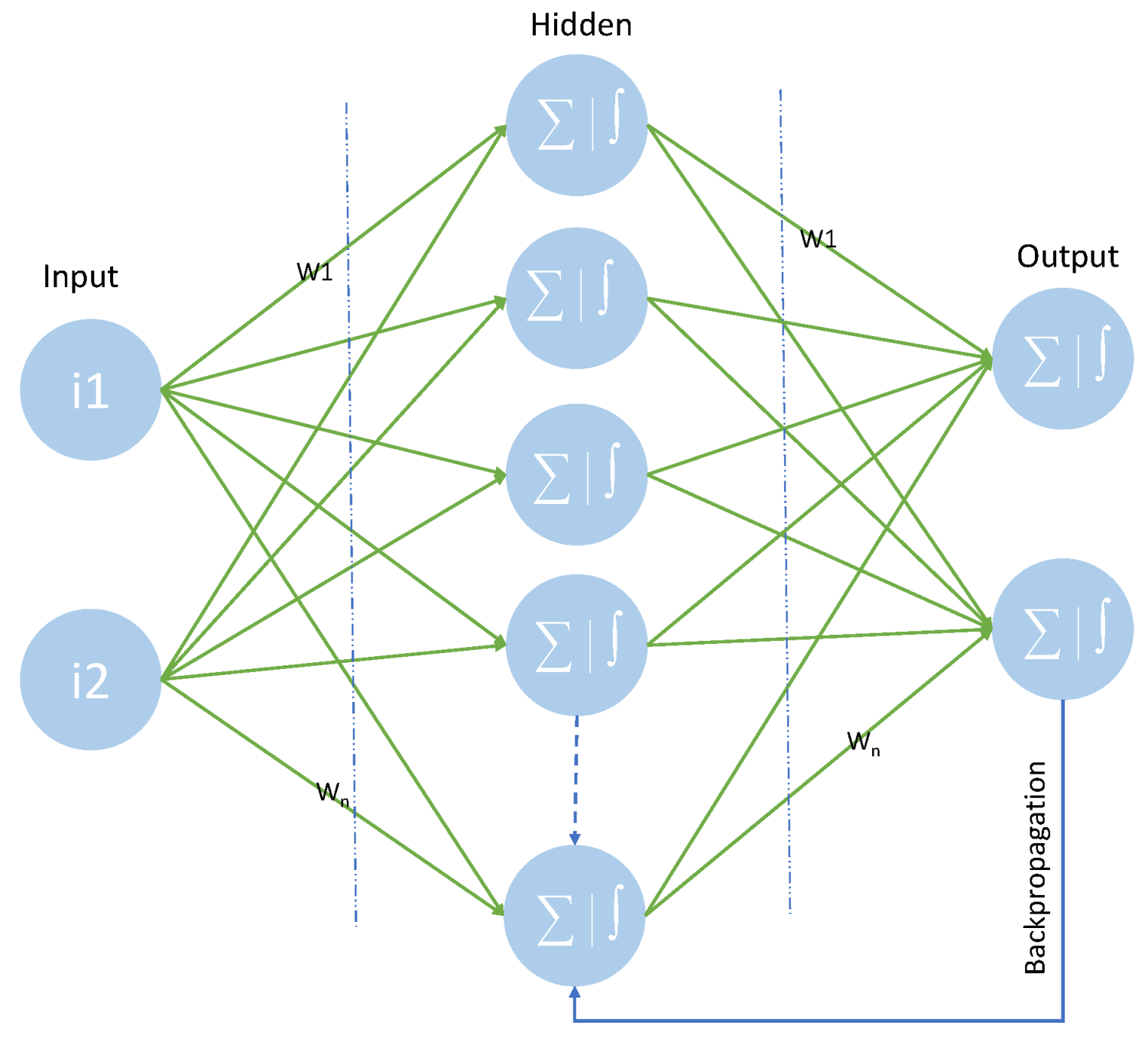
Artificial Neural Networks (ANNs) are computational models that emulate the human brain’s neural structure, functioning as universal function approximators. They typically consist of three primary layers: an input layer, several hidden layers, and an output layer. Each neuron or node within a layer connects to every neuron in the following layer, with the connection strength governed by adjustable parameters known as weight vectors. During training, the network continuously applies an optimization technique, aiming to reduce prediction errors by fine-tuning these parameters, thus enabling precise mapping of new input data to the appropriate output. These networks incorporate non-linear activation functions like Sigmoid, Tanh, or ReLU to reflect data’s non-linear characteristics, allowing ANNs to handle complex functions effectively and generalize well to diverse datasets. In this particular study, the Adaptive Moment Estimation (ADAM) algorithm was employed for optimizing the cost function, with ReLU selected as the activation function. The complete structure of ANN is shown in
Figure 3.
Consider a model with
H input neurons and
N neurons in a hidden layer. The
nth neuron in the hidden layer is determined by the weighted sum of the input layer neurons and a bias value. In a three-layer ANN, the values for the hidden layer neuron and output neuron are calculated using the following equations:
where
is the input value of the
jth neuron in the hidden layer,
is the weight between the
jth neuron in the hidden layer and the
ith neuron in the input layer,
is the
ith input variable of the input layer, and
is the bias term of the
jth neuron in the hidden layer. Different activation functions are employed to transform the output of the hidden layer neurons.
where
is the output of the
jth neuron in the hidden layer, and
f is the activation function, such as Sigmoid, Tanh, ReLU, etc.
where
is the output neuron, derived by taking the weighted sum of hidden layer neurons (
) and the bias term
of the output neuron. Based on a trial-and-error method, 128 hidden nodes with one hidden layer were employed in the development of ANN models.
4.4. Fuzzy Logic Controller
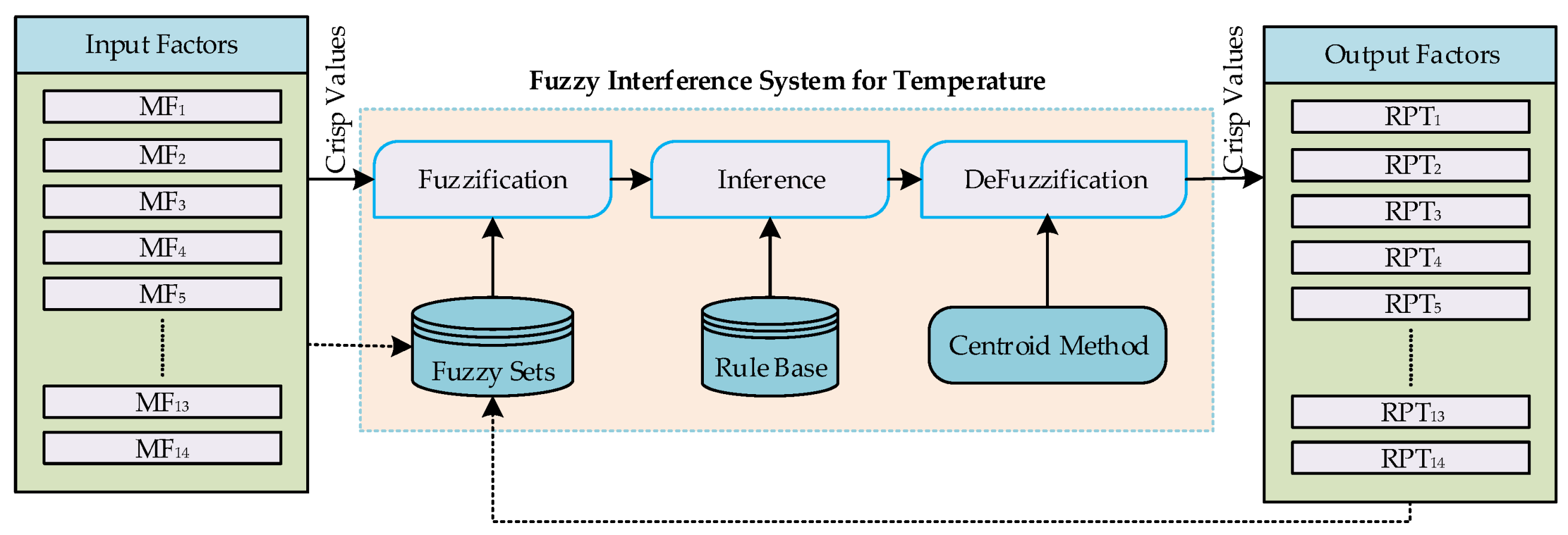
In the proposed research, a fuzzy controller has been employed to regulate power consumption, a common technique used in various applications. Fuzzy logic, a versatile and effective approach, has garnered significant attention from researchers across different fields. In this study, the Mamdani fuzzy logic method, known for its simplicity and efficacy, has been utilized. The Mamdani fuzzy logic model comprises three core components: fuzzification, rule inference, and defuzzification.
The fuzzification module converts crisp input values into fuzzy inputs by applying input membership functions. The rule inference module generates rules using input and output membership functions, while the defuzzification module employs the centroid method to convert fuzzy outputs into crisp values.
Table 1 shows the fuzzzy rules for power optimization, environmental quality and lighting management.
In this investigation, the triangular membership function has been adopted for both input and output membership functions. The mathematical representation of the triangular membership function is provided in Equation (
16).
In the realm of fuzzy logic control systems, three distinct controllers have been accurately designed, each designed for a specific application, and ruled by a set of membership functions. These functions play a pivotal role in mapping the input variables to appropriate output responses, enabling the controllers to handle complex, detailed scenarios.The operational process of Mamdani fuzzy logic is depicted in
Figure 4.
Table 2 shows the temperature fuzzy controller with 14 different combination of fuzzy rules.
The first controller, dedicated to power optimization, operates with the input variable labeled “Var_1” and an output variable known as “RPTemp.” This controller is specifically constructed to manage and optimize power usage efficiently. In its collection, it features fourteen unique membership functions for “Var_1,” each thoroughly labeled from Var_1_1 to Var_1_14. These functions allow the controller to interpret various levels of power requirements or conditions and correspondingly adjust the output, which is also finely segmented into fourteen membership functions, labeled RPTemp_1 through RPTemp_14. The roughness of these functions facilitates a highly detailed approach to power management, ensuring that the controller can respond with great precision to different power-related scenarios.
The second controller is at the controls of lighting management. This controller, encompassing the input variable “Var_2” and the output variable “RPILL,” is designed with a focus on regulating and optimizing lighting conditions. It employs an expanded set of twenty membership functions for “Var_2,” ranging from Var_2_1 to Var_2_20, offering a broad spectrum of input interpretation capabilities.
Similarly, the output variable “RPILL” is equipped with an equally diverse set of twenty membership functions. This expansive range allows the lighting management controller to adjust lighting levels with remarkable accuracy and responsiveness, offering a wide array of lighting conditions and preferences.
Table 3 shows the Illumination fuzzy controller with 20 different combination of fuzzy rules.
Lastly, the third controller is centered on environmental quality management. It utilizes “Var_3” as its input variable and “RPAQ” as the output variable. This controller is integral to monitoring and enhancing the quality of the environment. It is equipped with eighteen membership functions for “Var_3,” labeled from Var_3_1 to Var_3_18, which enable it to interpret various environmental factors effectively. The output variable “RPAQ” mirrors this with its own set of eighteen membership functions, from RPAQ_1 to RPAQ_18. The design of these functions allows the controller to make informed decisions about environmental adjustments, striving to maintain or improve the overall environmental quality.
Each of these controllers, with their respective sets of rules and membership functions, exemplifies the versatility and adaptability of fuzzy logic systems. By finely tuning the input and output variables through these functions, the controllers can handle complex, real-world scenarios with a degree of sophistication and accuracy. For a comprehensive understanding of how these controllers operate and interact with their respective variables, a detailed model is presented in Table 1. This table encapsulates the complex web of rules that govern the decision-making processes within these fuzzy logic systems.
Table 4 shows the air quality fuzzy controller with 18 different combination of fuzzy rules.
4.5. Coordinator Agent
The Coordinator Agent acts as a critical component in the smart home ecosystem, tasked with processing the outputs from the fuzzy logic controller to regulate environmental conditions. This includes managing the heating or cooling systems, lighting intensity, and CO2 levels to optimize occupant comfort and energy efficiency.
At the outset, the agent assesses two essential metrics: the remaining battery capacity of the home’s energy storage system and the estimated energy consumption based on current usage patterns. Should the projected energy consumption exceed what the stored battery capacity can deliver, the Coordinator Agent dynamically adjusts the power supply to the home’s actuators, engaging in an optimization loop to ensure energy is utilized effectively.
This process is carried out iteratively, sustaining the optimization as long as the energy storage can support the home’s operational demands.
Conversely, if the energy forecast indicates that the battery reserve is inadequate for anticipated needs, the optimization routine is promptly suspended to prevent energy depletion.
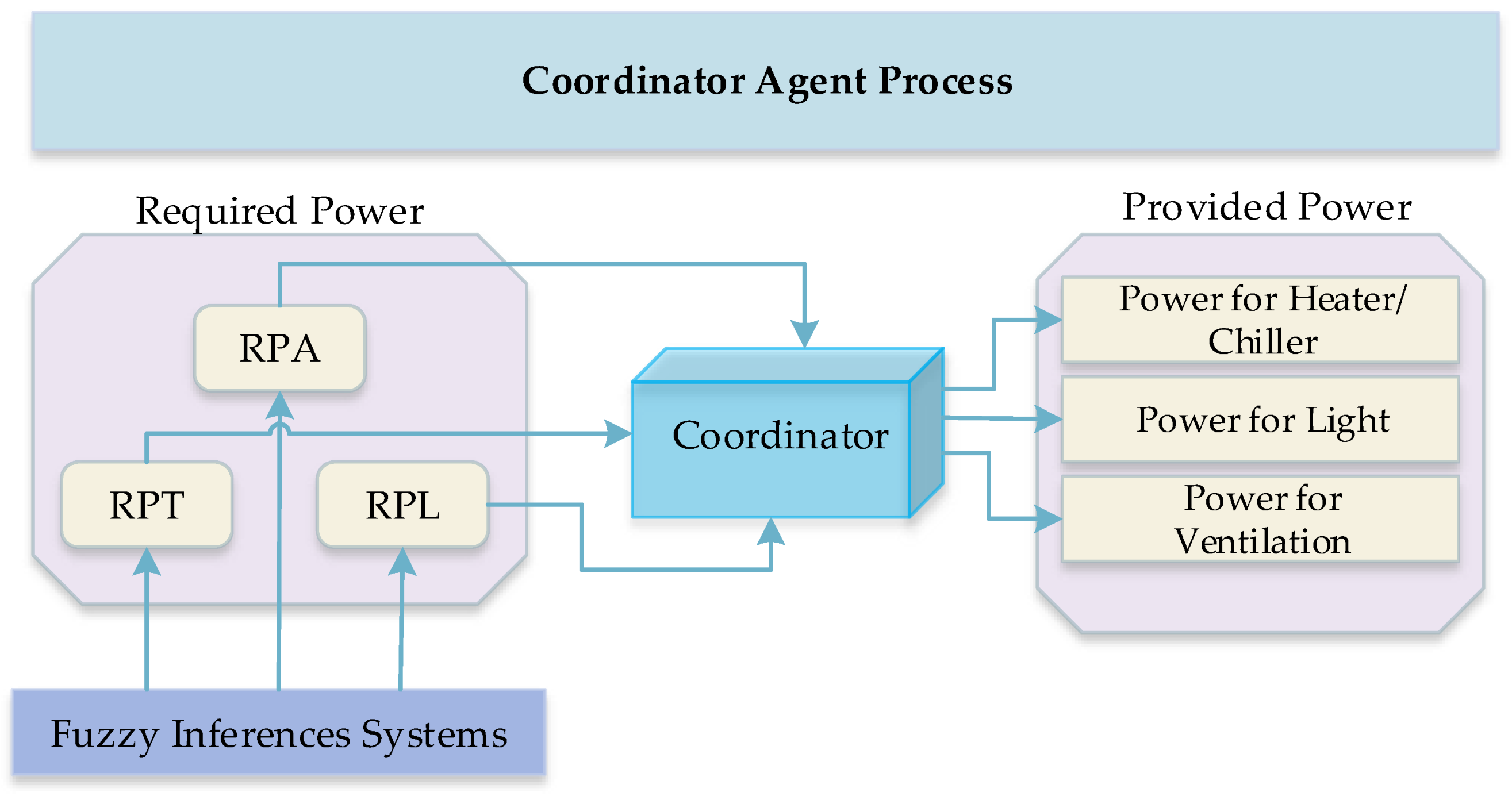
Figure 6 illustrates a comprehensive structural diagram of the
Coordinator Agent’s role and operational logic within the smart home infrastructure.
Figure 5 shows the both provide power and required power for coordinator agent.
4.6. Performance Evaluation
Various performance metrics are employed to assess the effectiveness of prediction algorithms. In this proposed study, performance indices such as Mean Absolute Error (MAE), Root Mean Square Error (RMSE), and Mean Absolute Percentage Error (MAPE) are utilized for comparing actual values with predicted values. The distribution of error minimization is quantified through Mean Squared Error (MSE). MAPE assesses the difference as a percentage of the target, while RMSE measures the error between the estimate and the target. The performance metrics, RMSE, MAE, and MAPE, can be expressed through the following equations:
Here, N denotes the total number of values, T represents the target value, and P signifies the estimated value. These performance metrics provide a comprehensive evaluation of the prediction algorithm by quantifying the accuracy and reliability of the predicted values in comparison to the actual values.
5. Experimental Results and Discussion
The proposed model is implemented on an 11th Gen Intel(R) Core(TM) i7-11700KF @ 3.60GHz, utilizing Python 3.12.0.
Table 5 provides details of the system configuration for implementation and simulation analysis.
The data utilized in this study is sourced from reference [
19], encompassing three factors: temperature, illumination, and air quality. For the temperature fuzzy logic controller, seven input and output rules are specified for input variable
and output variable
, respectively. Similarly, fifteen input and output rules are defined for the illumination fuzzy logic controller’s input variable
and output variable
. In the air quality fuzzy logic controller, fifteen input and output rules are specified for input variable
and output variable
.
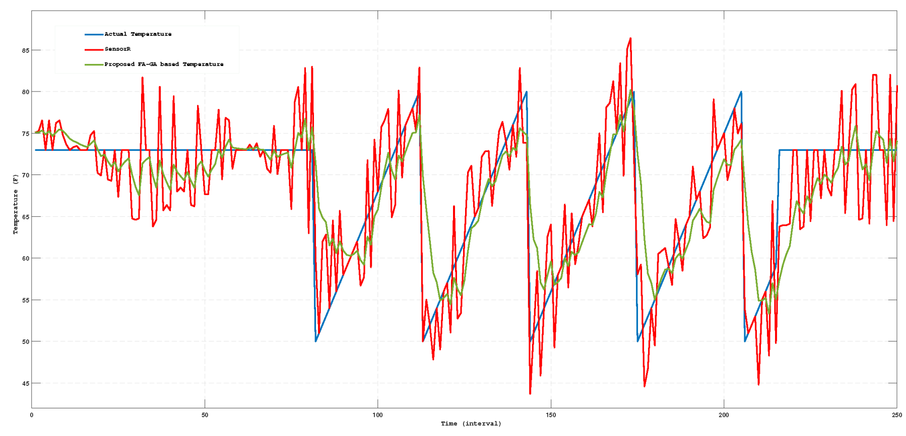
In the proposed approach, a Kalman filter is employed to smooth sensor reading data and eliminate outliers from input sensor data.
Figure 6 illustrates the actual temperature, sensor reading temperature, and predicted temperature. Likewise,
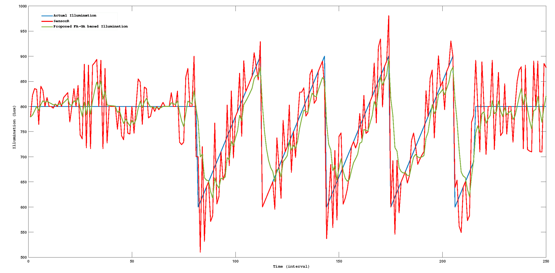
Figure 7 provides a detailed depiction of actual illumination, sensor illumination, and air quality illumination.
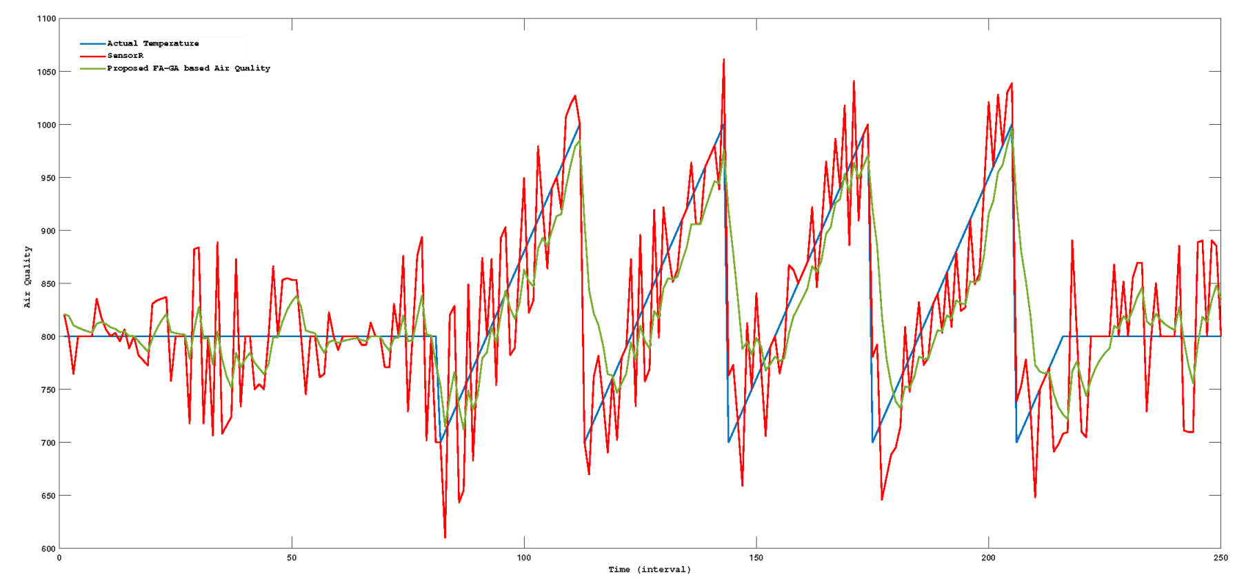
Figure 8 presents actual air quality, sensed air quality, and predicted air quality values.
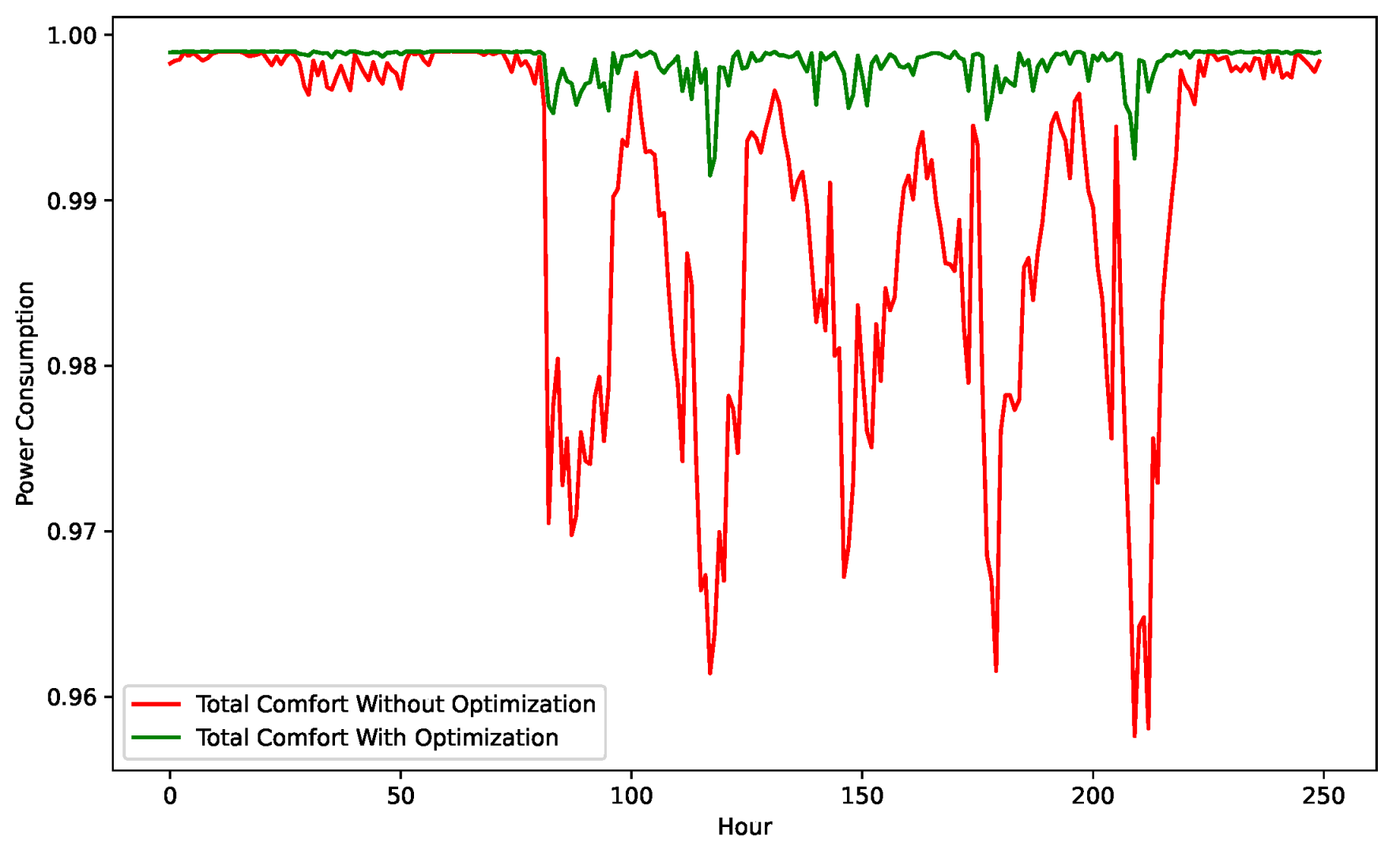
Figure 9 illustrates the comfort index levels in scenarios where both optimization techniques are applied and removed. it shows the total comfort with and without optimization. The depicted values are significantly removed from the optimal range, indicating a lower comfort index under typical conditions. On the other hand, the figure also showcases the comfort index levels when the proposed FA-GA optimization approaches are employed. Here, the majority of the values incline towards 1, denoting a higher comfort index. This comparison strongly suggests that the comfort index is considerably improved when the proposed optimization methods are utilized.
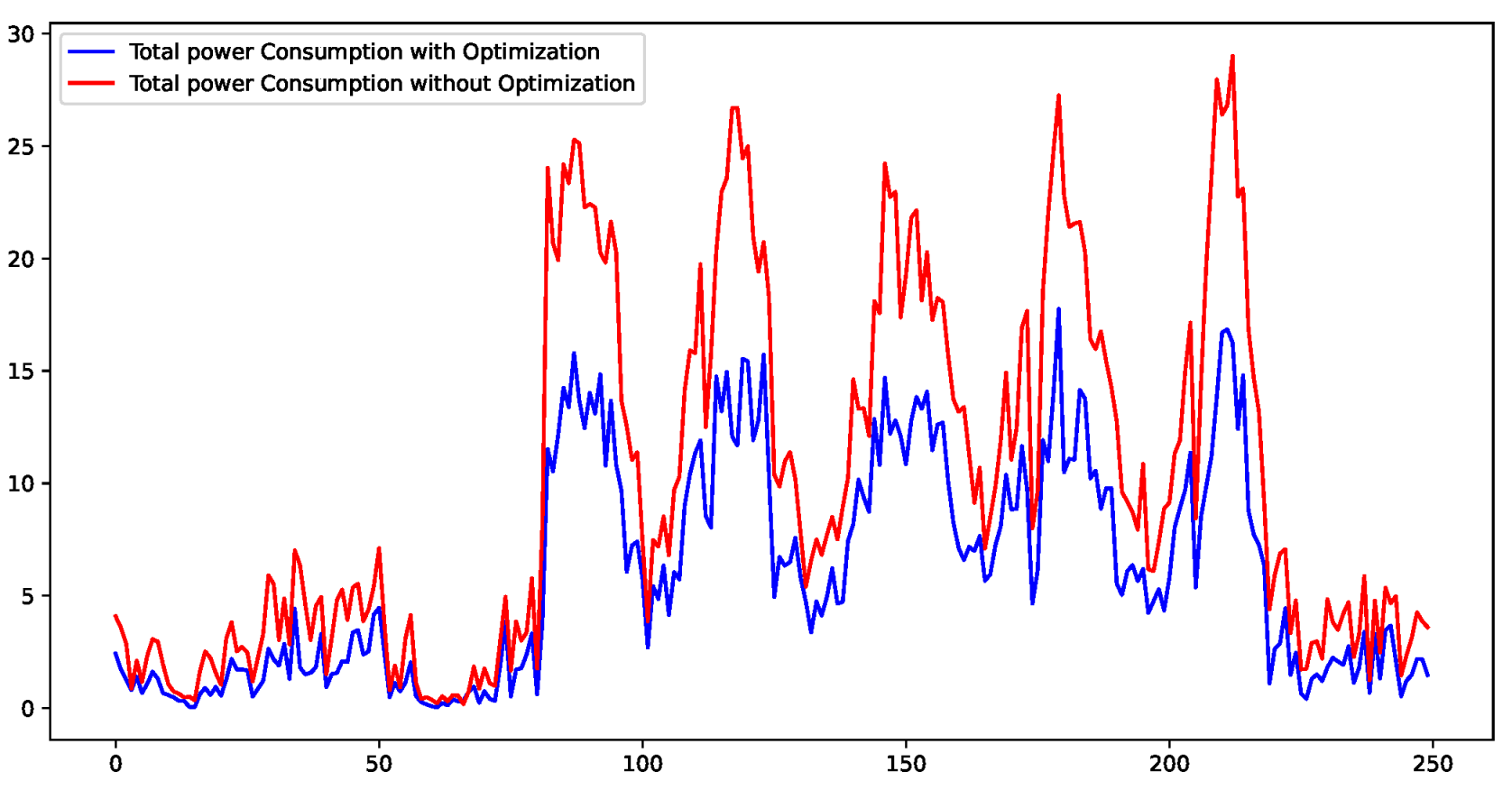
Figure 9 presents a comparison of how much electricity is used in two scenarios: one where an optimization scheme is applied and the other where no such scheme is used. The difference is noticeable; when the optimization scheme is in place, there’s a reduction in electricity usage compared to the scenario without it. This optimization scheme is what we are referring to as our proposed approach. It clearly demonstrates that adopting this scheme leads to more efficient energy use.
Figure 10 shows the power consumption with and without optimization scheme.
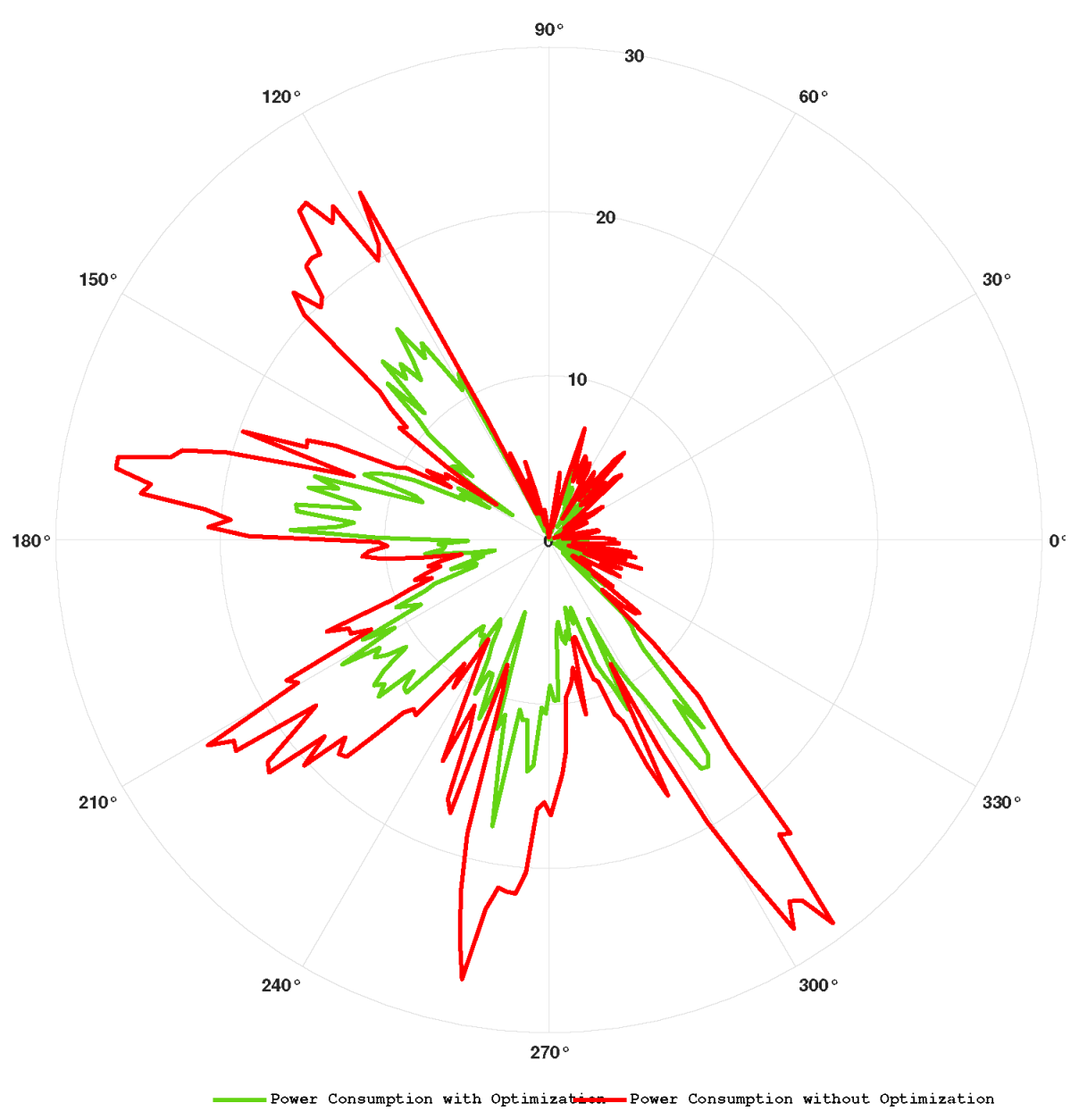
The radar chart depicted in
Figure 11 compares two datasets: `Power Consumption with Optimization,’ represented by a green line, and `Power Consumption without Optimization,’ depicted by a red line. The chart features multiple axes extending from a central point, each representing different conditions or categories that are crucial for illustrating variations in power consumption. When the green line is closer to the center, it indicates that optimization has effectively reduced power consumption. In contrast, when the red line is farther from the center, indicating higher power consumption, it suggests that optimization was less effective or did not lead to a reduction in power consumption.
5.1. Analysis of different Models
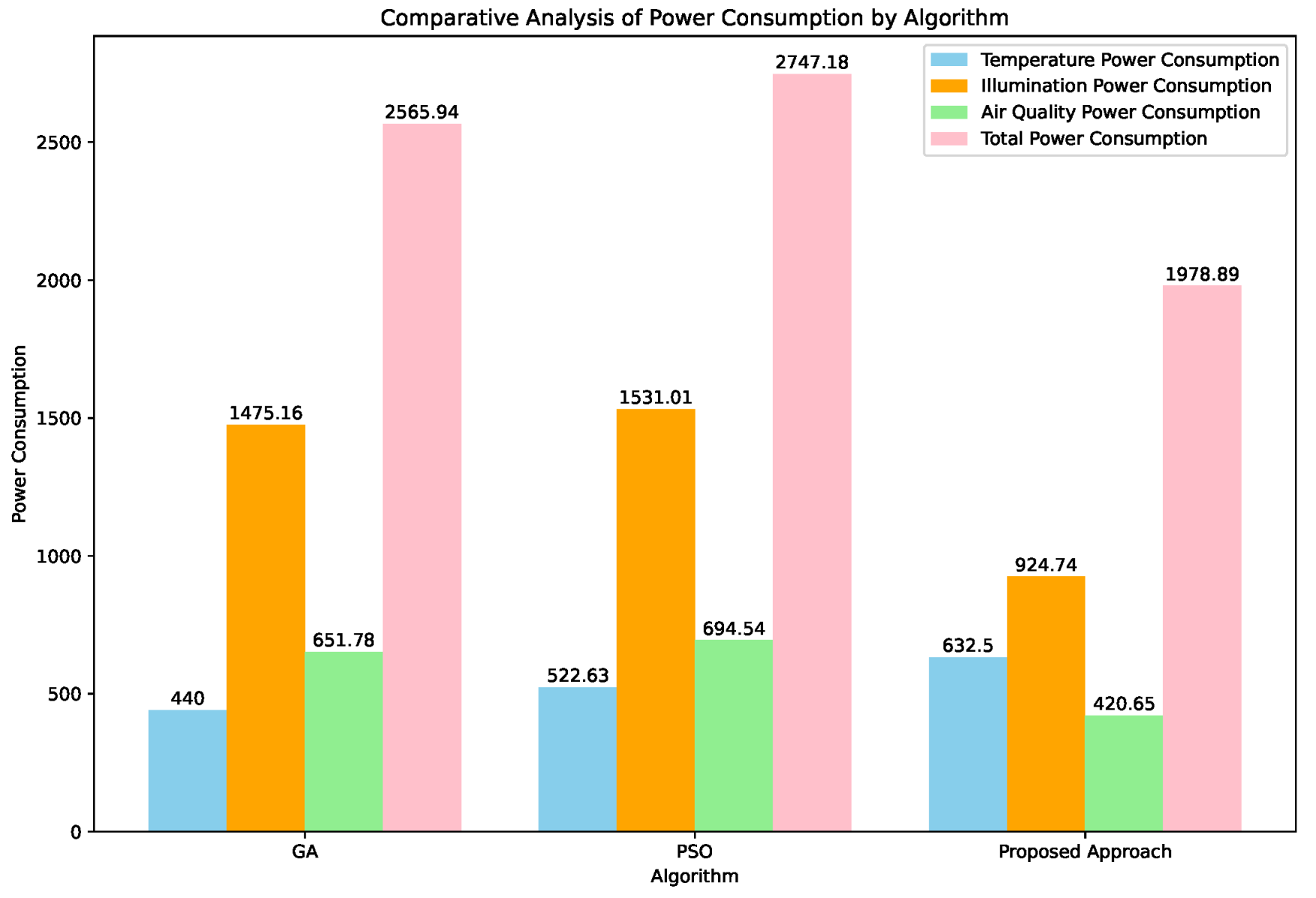
The comparative analysis conducted in this study critically evaluates a newly developed FA-GA method against existing, well-established methods. This evaluation, detailed in
Table 6 and
Figure 12, emphasizes both individual energy parameters and the overall consumption.
The results of this analysis clearly demonstrate that the new method offers enhanced efficiency in terms of energy usage compared to other known approaches. if we can see the detail values as defined in Table 6, we observe that the energy consumption for each algorithm is categorized into several key areas: Temperature, Illumination, and Air Quality Power Consumption, in addition to the Total Power Consumption. It’s noteworthy that while the new proposed approach records a slightly higher Temperature Power Consumption (632.5) than GA (440) and PSO (522.63), it shows remarkable efficiency in other areas. Particularly, in Illumination Power Consumption, the proposed method uses only 924.74 units of power, which is significantly lower compared to the 1475.16 and 1531.01 units consumed by GA and PSO, respectively. Similarly, for Air Quality Power Consumption, the new approach also demonstrates superior efficiency, utilizing just 420.65 units compared to GA’s 651.78 and PSO’s 694.54 units.
However, the most remarkable aspect of the analysis is the total energy consumption. The proposed approach has an overall consumption of only 1978.89 units, which is considerably lower than GA’s 2565.94 and PSO’s 2747.18 units. This comprehensive metric is critical as it represents the overall energy footprint of the algorithm. The significant reduction in total energy consumption with the new method, despite its higher usage in temperature adjustment, emphasizes its effectiveness in minimizing the overall energy footprint. This efficiency makes the proposed approach a more favorable option in scenarios where reducing energy consumption is vital.
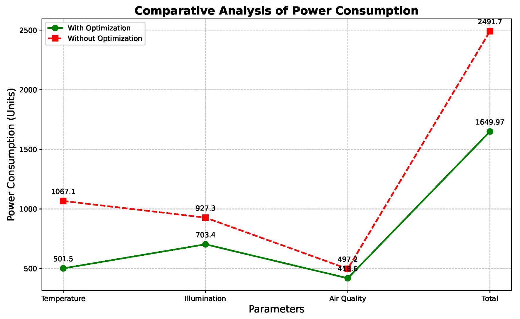
Table 7 and
Figure 13 presents a comparative analysis of power consumption for different environmental parameters with and without the application of optimization techniques. The parameters evaluated include temperature, illumination, and air quality. For each parameter, the power consumption is significantly lower when optimization is applied: 501.5 vs. 1067.1 units for temperature, 703.4 vs. 927.3 units for illumination, and 418.6 vs. 497.2 units for air quality. The total power consumption shows a marked decrease from 2491.7 units without optimization to 1649.97 units with optimization, highlighting the impact and benefit of employing energy-saving measures.
The
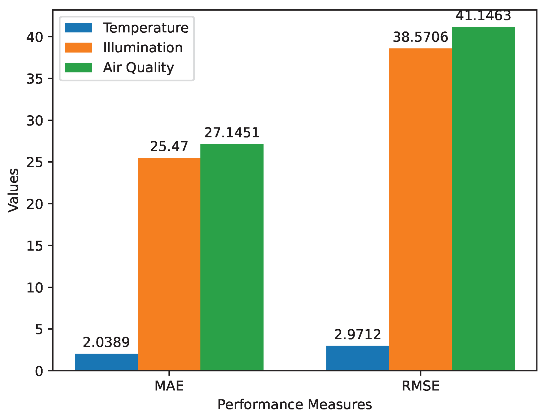
Table 8 and
Figure 14 presents a comprehensive performance evaluation of an optimization algorithm applied to three distinct environmental parameters: Temperature, Illumination, and Air Quality.
The evaluation is based on two key performance measures: Mean Absolute Error (MAE) and Root Mean Square Error (RMSE). For Temperature, the MAE is 2.0389, indicating relatively accurate predictions. Similarly, RMSE measures the algorithm’s predictive accuracy by calculating the root mean square of the prediction errors. For Illumination and Air Quality, the RMSE values are 38.5706 and 41.1463, respectively, suggesting slightly larger prediction errors compared to Temperature.
Figure 1.
Conceptual structure diagram of the proposed model.
Figure 1.
Conceptual structure diagram of the proposed model.
Figure 2.
Detailed proposed schematic diagram.
Figure 2.
Detailed proposed schematic diagram.
Figure 3.
Complete ANN structure.
Figure 3.
Complete ANN structure.
Figure 4.
Operational process of Mamdani fuzzy logic
Figure 4.
Operational process of Mamdani fuzzy logic
Figure 5.
Provide power and required power for coordinator agent.
Figure 5.
Provide power and required power for coordinator agent.
Figure 6.
Actual temperature, sensor reading temperature, and predicted temperature
Figure 6.
Actual temperature, sensor reading temperature, and predicted temperature
Figure 7.
Actual illumination, sensor illumination, and air quality illumination
Figure 7.
Actual illumination, sensor illumination, and air quality illumination
Figure 8.
Actual air quality, sensed air quality, and predicted air quality values
Figure 8.
Actual air quality, sensed air quality, and predicted air quality values
Figure 9.
Total comfort index with and without optimization.
Figure 9.
Total comfort index with and without optimization.
Figure 10.
Total power consumption with and without optimization.
Figure 10.
Total power consumption with and without optimization.
Figure 11.
Total power consumption with and without optimization.
Figure 11.
Total power consumption with and without optimization.
Figure 12.
Comparative analysis of different models.
Figure 12.
Comparative analysis of different models.
Figure 13.
Fuzzy logic based comparative Analysis of Power Consumption With and Without Optimization.
Figure 13.
Fuzzy logic based comparative Analysis of Power Consumption With and Without Optimization.
Figure 14.
comparative Analysis with MAE and RMSE.
Figure 14.
comparative Analysis with MAE and RMSE.
Table 1.
FUZZY RULES FOR POWER OPTIMIZATION, LIGHTING MANAGEMENT, AND ENVIRONMENTAL QUALITY FUZZY CONTROLLERS
Table 1.
FUZZY RULES FOR POWER OPTIMIZATION, LIGHTING MANAGEMENT, AND ENVIRONMENTAL QUALITY FUZZY CONTROLLERS
| Fuzzy Controller 1: |
Fuzzy Controller 2: |
Fuzzy Controller 3: |
| Rules for Power |
Rules for Lighting |
Rules for Environmental |
| Optimization |
Management |
Quality |
| Input "Var_1" |
Input "Var_2" |
Input "Var_3" |
| Output "RPTemp" |
Output "RPILL" |
Output "RPAQ" |
| Var_1_1 → RPTemp_1 |
Var_2_1 → RPILL_1 |
Var_3_1 → RPAQ_1 |
| Var_1_2 → RPTemp_2 |
Var_2_2 → RPILL_2 |
Var_3_2 → RPAQ_2 |
| Var_1_3 → RPTemp_3 |
Var_2_3 → RPILL_3 |
Var_3_3 → RPAQ_3 |
| Var_1_4 → RPTemp_4 |
Var_2_4 → RPILL_4 |
Var_3_4 → RPAQ_4 |
| Var_1_5 → RPTemp_5 |
Var_2_5 → RPILL_5 |
Var_3_5 → RPAQ_5 |
| Var_1_6 → RPTemp_6 |
Var_2_6 → RPILL_6 |
Var_3_6 → RPAQ_6 |
| Var_1_7 → RPTemp_7 |
Var_2_7 → RPILL_7 |
Var_3_7 → RPAQ_7 |
| Var_1_8 → RPTemp_8 |
Var_2_8 → RPILL_8 |
Var_3_8 → RPAQ_8 |
| Var_1_9 → RPTemp_9 |
Var_2_9 → RPILL_9 |
Var_3_9 → RPAQ_9 |
| Var_1_10 → RPTemp_10 |
Var_2_10 → RPILL_10 |
Var_3_10 → RPAQ_10 |
| Var_1_11 → RPTemp_11 |
Var_2_11 → RPILL_11 |
Var_3_11 → RPAQ_11 |
| Var_1_12 → RPTemp_12 |
Var_2_12 → RPILL_12 |
Var_3_12 → RPAQ_12 |
| Var_1_13 → RPTemp_13 |
Var_2_13 → RPILL_13 |
Var_3_13 → RPAQ_13 |
| Var_1_14 → RPTemp_14 |
Var_2_14 → RPILL_14 |
Var_3_14 → RPAQ_14 |
| – |
Var_2_15 → RPILL_15 |
Var_3_15 → RPAQ_15 |
| – |
Var_2_16 → RPILL_16 |
Var_3_16 → RPAQ_16 |
| – |
Var_2_17 → RPILL_17 |
Var_3_17 → RPAQ_17 |
| – |
Var_2_18 → RPILL_18 |
Var_3_18 → RPAQ_18 |
| – |
Var_2_19 → RPILL_19 |
– |
| – |
Var_2_20 → RPILL_20 |
– |
Table 2.
Temperature Fuzzy Controller Fuzzy Rules
Table 2.
Temperature Fuzzy Controller Fuzzy Rules
| Symbol |
Range |
Symbol |
Range |
| Var_1_1
|
|
RPTemp_1
|
|
| Var_1_2
|
|
RPTemp_2
|
|
| Var_1_3
|
|
RPTemp_3
|
|
| Var_1_4
|
|
RPTemp_4
|
|
| Var_1_5
|
|
RPTemp_5
|
|
| Var_1_6
|
|
RPTemp_6
|
|
| Var_1_7
|
|
RPTemp_7
|
|
| Var_1_8
|
|
RPTemp_8
|
|
| Var_1_9
|
|
RPTemp_9
|
|
| Var_1_10
|
|
RPTemp_10
|
|
| Var_1_11
|
|
RPTemp_11
|
|
| Var_1_12
|
|
RPTemp_12
|
|
| Var_1_13
|
|
RPTemp_13
|
|
|
Var_1_14
|
|
RPTemp_14
|
|
Table 3.
Illumination Fuzzy Controller Fuzzy Rules
Table 3.
Illumination Fuzzy Controller Fuzzy Rules
| Symbol |
Range |
Symbol |
Range |
|
Var_2_1
|
|
RPILL_1
|
|
|
Var_2_2
|
|
RPILL_2
|
|
|
Var_2_3
|
|
RPILL_3
|
|
|
Var_2_4
|
|
RPILL_4
|
|
|
Var_2_5
|
|
RPILL_5
|
|
|
Var_2_6
|
|
RPILL_6
|
|
|
Var_2_7
|
|
RPILL_7
|
|
|
Var_2_8
|
|
RPILL_8
|
|
|
Var_2_9
|
|
RPILL_9
|
|
|
Var_2_10
|
|
RPILL_10
|
|
|
Var_2_11
|
|
RPILL_11
|
|
|
Var_2_12
|
|
RPILL_12
|
|
|
Var_2_13
|
|
RPILL_13
|
|
|
Var_2_14
|
|
RPILL_14
|
|
|
Var_2_15
|
|
RPILL_15
|
|
|
Var_2_16
|
|
RPILL_16
|
|
|
Var_2_17
|
|
RPILL_17
|
|
|
Var_2_18
|
|
RPILL_18
|
|
|
Var_2_19
|
|
RPILL_19
|
|
|
Var_2_20
|
|
RPILL_20
|
|
Table 4.
Air Quality Fuzzy Controller Fuzzy Rules
Table 4.
Air Quality Fuzzy Controller Fuzzy Rules
| Symbol |
Range |
Symbol |
Range |
|
Var_3_1
|
|
RPAQ_1
|
|
|
Var_3_2
|
|
RPAQ_2
|
|
|
Var_3_3
|
|
RPAQ_3
|
|
|
Var_3_4
|
|
RPAQ_4
|
|
|
Var_3_5
|
|
RPAQ_5
|
|
|
Var_3_6
|
|
RPAQ_6
|
|
|
Var_3_7
|
|
RPAQ_7
|
|
|
Var_3_8
|
|
RPAQ_8
|
|
|
Var_3_9
|
|
RPAQ_9
|
|
|
Var_3_10
|
|
RPAQ_10
|
|
|
Var_3_11
|
|
RPAQ_11
|
|
|
Var_3_12
|
|
RPAQ_12
|
|
|
Var_3_13
|
|
RPAQ_13
|
|
|
Var_3_14
|
|
RPAQ_14
|
|
|
Var_3_15
|
|
RPAQ_15
|
|
|
Var_3_16
|
|
RPAQ_16
|
|
|
Var_3_17
|
|
RPAQ_17
|
|
|
Var_3_18
|
|
RPAQ_18
|
|
Table 5.
Simulation Configuration
Table 5.
Simulation Configuration
| Tool |
Specification |
| CPU |
Intel(R) Core (TM) i5-3570 |
| |
@ 3.40 GHz |
| RAM |
16 GB |
| Graphics |
NVIDIA GeForce 9600 GT |
| Operating System |
Windows 10 |
| Programming Tool |
Matlab 2018a |
Table 6.
Comparative analysis of different models
Table 6.
Comparative analysis of different models
| Parameters |
GA |
PSO |
Proposed
Approach |
Temperature
Power Consumption
|
440 |
522.63 |
632.5 |
Illumination
Power Consumption
|
1475.16 |
1531.01 |
924.74 |
Air Quality
Power Consumption
|
651.78 |
694.54 |
420.65 |
Total
Power Consumption
|
2565.94 |
2747.18 |
1978.89 |
Table 7.
Fuzzy logic based comparative Analysis of Power Consumption With and Without Optimization
Table 7.
Fuzzy logic based comparative Analysis of Power Consumption With and Without Optimization
| Parameters |
With |
Without |
| |
Optimization |
Optimization |
| Temperature |
501.5 |
1067.1 |
| Power Consumption |
|
|
| Illumination |
703.4 |
927.3 |
| Power Consumption |
|
|
| Air Quality |
418.6 |
497.2 |
| Power Consumption |
|
|
| Total |
1649.97 |
2491.7 |
| Power Consumption |
|
|
Table 8.
The performance measurement of optimization algorithm for temperature, illumination, and air quality
Table 8.
The performance measurement of optimization algorithm for temperature, illumination, and air quality
| Performance |
Temperature |
Illumination |
Air Quality |
| Measures |
|
|
|
| MAE |
2.0389 |
25.47 |
27.1451 |
| RMSE |
2.9712 |
38.5706 |
41.1463 |
