High-Speed 3D Printing Temperature Control with Optimized PID Parameters Based on Improved ALO Algorithm

1. Introduction

Fused deposition modeling (FDM) technology, a widely used and promising three-dimensional (3D) printing technology [1], is rapidly growing. High-speed FDM 3D printing is favored for its fast printing speed, networked control, parameter visualization, among other features. During the use of high-speed FDM 3D printing, though, it is found that it takes a relatively lengthy period of time for users to wait for the nozzle to heat up, and that real-time monitoring of the print nozzle temperature jitter is becoming increasingly serious in the 3D printing process.

The quality of 3D printed part is significantly affected by the speed of printing and nozzle temperature [2]. Although with optimization algorithms such as fuzzy control [3], model predictive control [4] and robust control [5] have emerged in the field of 3D printing temperature control with the development of technology and advanced control strategies, The temperature control of FDM 3D printing in practical applica-tions is still dominated by the proportional-integral-derivative (PID) control meth-od,which is simple in principle as well as in structure, and is thereby widely used for a wide range of problems: process control, magnetic and optic memories, automo-tive,etc [6]. Traditional PID control methods have certain limitations in the face of complex nonlinear systems due to the nonlinearity and hysteresis of the actual temperature during the heating and printing process of the FDM 3D printing nozzle.

The ant-lion algorithm (ALO),as a new type of intelligent algorithm with good robustness and strong optimization-seeking ability, can effectively solve the stability problems occurring in the temperature control of high-speed FDM 3D printing,and has been adopted in various professions [7,8,9]. Nevertheless, the ALO algorithm needs to be improved because it still has the problem of relying too much on the initial solution, the elitist efficiency is not high, and it is easy to fall into the local optimization. Nowa-days, there are scholars who have achieved superior outcomes by improving the ALO algorithm for diverse tasks. Li [10] and others developed a Gaussianmutation based ALO (GALO) algorithm and applied it to the 0-1 backpack problem. In order to accurately and efficiently diagnose the health state of rolling bearings, Wang [11] proposed a rolling bearing fault diagnosis model based on Improved Antli-on Optimization (IALO) algorithm to optimize BP neural network. Jie Ji [12] et al. in-vestigated the equipment capacity allocation of a chemical company’s cogeneration system for cooling, heating and power generation based on the improvement of ant-lion optimization algorithm by increasing the weight coefficients(WALO).

Considering the high requirements of high-speed FDM 3D printing on temperature control accuracy and stability, a 3D printing nozzle temperature control algorithm based on an improved ant-lion optimisation algorithm to optimize the PID parameters is presented in response to the problems in the above literature. Unlike other improved algorithms, the algorithm not only improves it from the perspectives of population initialisation and elitist formulae, which improves its search accuracy, convergence speed and stability, but also improves the existing chaotic mapping and proposes a Tent-Logistic-Cotangen composite mapping method, which effectively overcomes the characteristics of ALO that is prone to fall into local optimum and does not increase the time complexity of the algorithm, which has certain novelty. Finally, the method is applied to the MatLab high-speed 3D printing temperature simulation experiment and the semi-physical platform based on the Klipper firmware, which verifies the effectiveness and feasibility of the method.

2. Proposed Optimization

2.1. Traditional ALO

Ant Lion Optimizer (Ant Lion Optimizer) [13] is a natural heuristic algorithm proposed by Australian scholar Seyedali inspired by the hunting mechanism of ant li-ons in nature The core idea of the algorithm is to simulate the hunting mechanism of ant lions hunting ants in order to achieve the global optimization. The ant lion utilizes its traps dug into the sand in the shape of a funnel and hides at the bottom of the trap to wait for the hunting objects to approach the trap, once the ants engaging in random wandering behaviors fall into the trap, the ant lion would imme-diately capture and feed on them. After predation is complete, the funnel-shaped trap will be repaired and the next predation will take place.Interventionary studies involv-ing animals or humans, and other studies that require ethical approval, must list the authority that provided approval and the corresponding ethical approval code. As the movement of ants is stochastic, random walking is used to simulate the mobility of ants and the mathematical formulas describing the coordinates of their activities are as follows:

$${\mathrm{X}}_{\mathrm{i},\mathrm{j}}^{\mathrm{t}}=\left[0,\mathrm{cumsum}\left(2r\left(t_1\right)-1\right),\dots ,\mathrm{cumsum}\left(2r\left(t_n\right)-1\right)\right]$$

(1)

$$r\left(t\right)=\left\{\begin{array}{cc}1\hfill & \mathrm{if}\mathrm{rand}>0.5\hfill \\ 0\hfill & \mathrm{if}\mathrm{rand}⩽0.5\hfill \end{array}\right.$$

(2)

where ${\mathrm{X}}_{\mathrm{i},\mathrm{j}}^{\mathrm{t}}$is the position of each individual ant, t represents the current number of iterations, $cumsum\left(\right)$ denotes the cumulative sum of the randomized wandering steps,n is the maximum number of wandering times,$t_n$is the current number of iterations, and $r\left(t\right)$ is a random function, $rand$ is the random number, and $rand\in [0,1]$. Ant lions update their position to the prevailing location of the ant being hunted to enhance their opportunities to capture fresh pre-existing prey. The ant-lion is constantly updating its position through Equation (3).

$$\begin{array}{cc}\hfill & {\mathrm{Antlion}}_i^t={\mathrm{Ant}}_i^t\hfill \\ \hfill & \mathrm{if}f\left({\mathrm{Ant}}_i^t\right)>f\left({\mathrm{Antlion}}_i^t\right)\hfill \end{array}$$

(3)

where $\mathrm{f}\left({\mathrm{Ant}}_i^t\right)$ and $f\left({\mathrm{Antlion}}_i^t\right)$ are the fitness values of the ith-dimensional ants and ant-lion at the tth iteration, and ${Ant}_i^t$ and ${Antlion}_i^t$are the positions of the ith-dimensional ants and ant lion at the tth iteration. The Elite Strategy ensures that the optimal solution is obtained at any stage of the optimization process, and the best adapted ant lion in each iteration is reserved as the Elite Ant Lion, and each ant would select an Elite Ant Lion depending on the Roulette Strategy and the Elite Strategy, around which it would wandering randomly. Ants keep updating their position through Equation (4).

$$An{t}_i^t=\frac{R_A^t+R_E^t}{2}$$

(4)

where$R_A^t$is the position where the ants randomly walk around the antlion selected by roulette, and$R_E^t$is the position where the ants randomly walk around the elite antlion.

Ant Lion Optimizer (ALO) is a robust intelligent algorithm inspired by the hunting mechanism of ant lions in nature. Despite its strengths, it has drawbacks such as a lack of population diversity and a tendency to converge to local optima, necessitating improvements for more effective applications.

2.2. Classical chaotic mappings initialize populations

The traditional ALO algorithm employed random initialisation of the population, which tends to produce an inhomogeneous distribution of the initialised population and is not conducive to covering further areas in the search space. By taking a chaotic initialisation method to initialise the population, the coverage as well as the diversity can be increased. At present, the most commonly used methods of chaotic initialisation are logistic mapping, sine mapping,tent mapping and so on.

$$\mathrm{Logistic}\mathrm{map}:x_{i+1}=4r{x}_i\left(1-x_i\right)$$

(5)

$$\mathrm{Sin}\mathrm{e}\mathrm{map}:x_{i+1}=rsin\left(\pi x_i\right)$$

(6)

$$\mathrm{Tent}\mathrm{map}:x_{i+1}=\left\{\begin{array}{cc}2r{x}_i\hfill & \mathrm{if}{x}_i<0.5\hfill \\ 2r\left(1-x_i\right)\hfill & \mathrm{if}{x}_i\ge 0.5\hfill \end{array}\right.$$

(7)

Combining a diversity of low-dimensional chaos to form a new composite chaotic system. This type of chaotic system can effectively overcome the shortcomings of low-dimensional chaos, and is less complex and can be realised more conveniently than high-dimensional chaos.Tent-Logistic-Cosine chaos mapping utilises the existing Logistic, Sine and Tent maps as seed maps [14] as in Equation(8).

$$x_{i+1}=\left\{\begin{array}{cc}cos\left(\pi \left(2r{x}_i+4(1-r)x_i\left(1-x_i\right)-0.5\right)\right)\hfill & \mathrm{for}{x}_i<0.5;\hfill \\ cos\left(\pi \left(2r\left(1-x_i\right)+4(1-r)x_i\left(1-x_i\right)-0.5\right)\right)\hfill & \mathrm{for}{x}_i\ge 0.5,\hfill \end{array}\right.$$

(8)

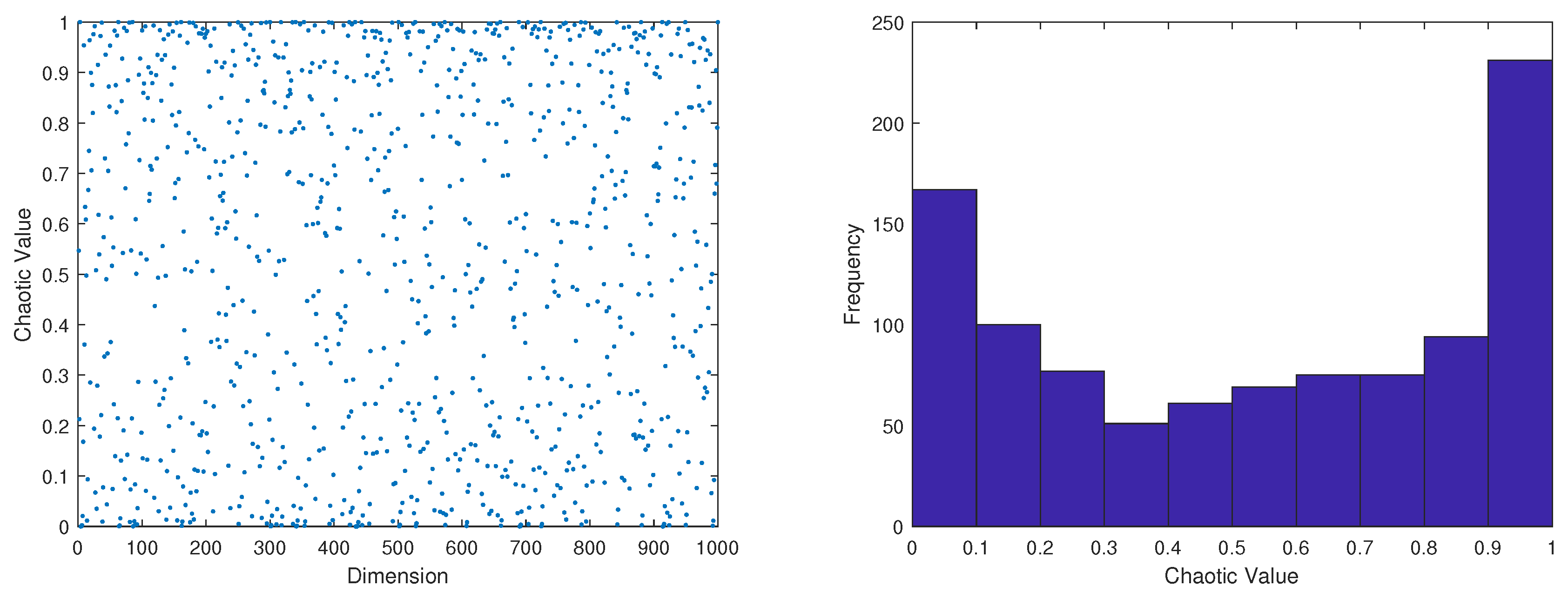
The distribution (left) and histogram (right) of the 1000 generations of Tent-Logistic-Cosine chaos mapping were generated on MATLAB as shown in Figure 2

Figure 1. (a)Chaotic sequence distribution diagram. (b) Histogram of distribution of chaotic sequence.

Figure 1. (a)Chaotic sequence distribution diagram. (b) Histogram of distribution of chaotic sequence.

The above figure shows that the sequence generated by the iteration of Tent-Logistic-Cosine chaotic mapping is not distributed uniformly in the phase space, meanwhile its parameter space in the chaotic state is narrower, and the chaotic effect is less effective.

2.3. Improved ALO

To address the above problems of traditional ALO, this paper improves the algorithm by introducing improved composite chaotic mapping and Elite Opposition-Based learning to initiate the population and increase the diversity of the population.

2.3.1. Tent-Logistic-Cotangent composite chaotic mapping

To avoid the existence of small circles and unstable points in the chaotic mapping, the periodicity, ergodicity and regularity of the chaotic variables are maintained.In this paper, we present a new chaotic mapping, named Tent-Logistic-Cotangent composite mapping, with the mathematical expression as in Equation (9).

$$x_{i+1}=\left\{\begin{array}{cc}mod(\left(\pi \left(rcot\left(4\pi x_i\right)+4(1-r)x_i\left(1-x_i\right)-0.2\right)\right),1)\hfill & \mathrm{for}{x}_i<0.5;\hfill \\ mod(\left(\pi \left((1-r)cot\left(4\pi x_i\right)+4(1-r)x_i\left(1-x_i\right)-0.15\right)\right),1)\hfill & \mathrm{for}{x}_i\ge 0.5,\hfill \end{array}\right.$$

(9)

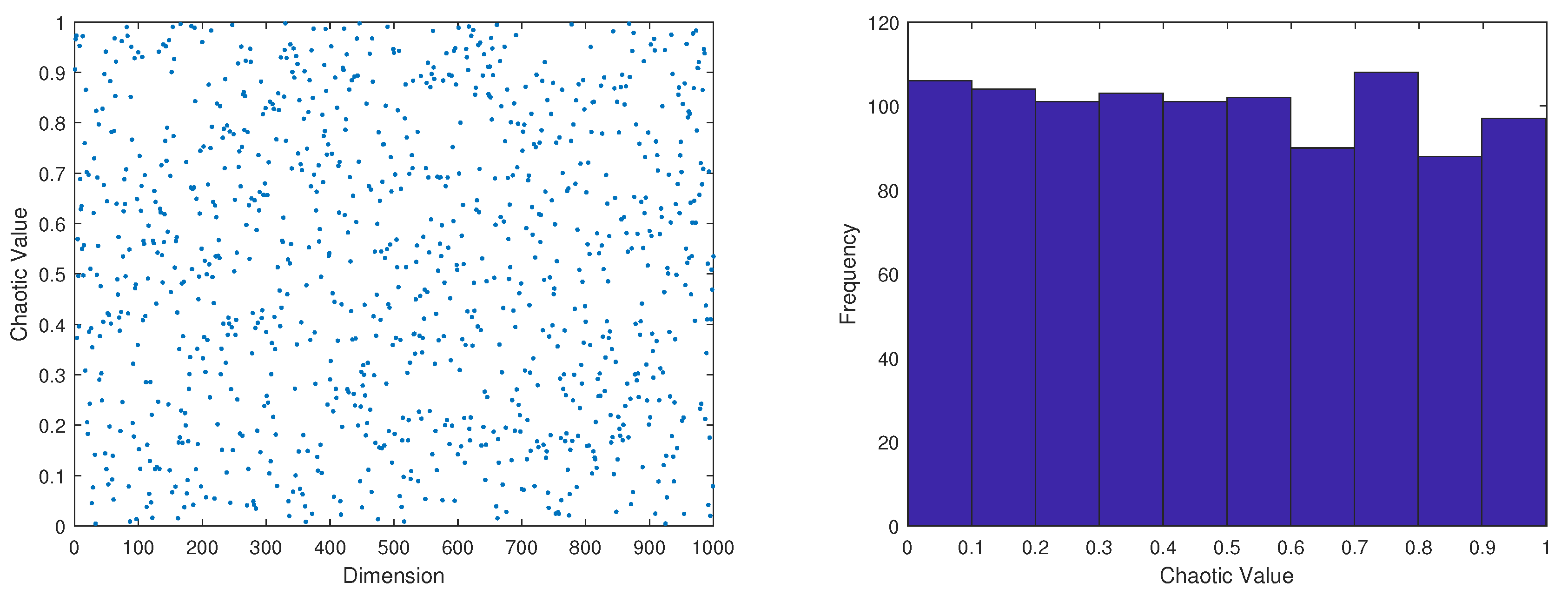
In contrast to Equation (8),the distribution (left) and histogram (right) of the 1000 generations of Tent-Logistic-Cotangent chaos mapping were also generated on MATLAB as shown in Figure 2.

Figure 2. (a)Tent-Logistic-Cotangent chaotic sequence distribution diagram. (b) Histogram of distribution of chaotic sequence.

Figure 2. (a)Tent-Logistic-Cotangent chaotic sequence distribution diagram. (b) Histogram of distribution of chaotic sequence.

Comparing Figure 1 and Figure 2, the proposed Tent-Logistic-Cotangent composite chaotic mapping iteration produces sequences that are more uniformly distributed in the phase space with excellent ergodicity.

2.3.2. Elite Opposition-Based learning

Opposition-Based Learning (OBL) is a machine intelligence strategy proposed by Tizhoosh [15] in 2005, and is used effectively to improve the quality of the solution by applying it to initialize the population. Elite Opposition-Based learning (EOBL) can improve on the basis of Opposition-Based Learning [16] , which extracts the elite individuals in the population in order to calculate the reverse individuals, and then select the candidate solutions with superior fitness values from the candidates.

Due to the great chance and blindness of the solutions generated by chaotic mapping, the generated solutions are subjected to Elite Opposition-Based learning to save convergence time and improve the quality of the solutions.It has been shown that real-world engineering problems have been solved by Elite Opposition-Based learning [17] .

Thus the elite backward learning based update initialization of the formulation as in Equation (10).

$$X_{i,j}^{t+2}=k\ast (lb+ub)-X_{i,j}^{t+1}$$

(10)

where $k\in [0,1]$. $lb$ is the lower bound of the solution space. $ub$ is the upper bound of the solution space.

2.3.3. Introduction of Cosine Factor Strategy

Traditional ALO algorithms later stage ant individuals perform random wandering towards ill-adapted ant lions, which can lead to weak iterative results and local optimum stagnation problems.Therefore, the cosine factor is introduced into the elitist update formula for adjusting the search direction to be closer to the direction of the optimization goal, and the algorithm is more exploratory, better avoids falling into the local optimum, and approaches the global optimum solution faster during the search process.Inspired by the cultural-particle swarm optimization algorithm (C-PSO) [18] , the algorithm uses adaptive inertia weights to balance global and local search capabilities.

Based on this, this paper designs a cosine factor for a given parameter can effectively reduce the situation of falling into the local optimum, and improve the search ability of local development and global,as in equations (11)-(12).

$$\theta \left(k\right)={\omega }_{min}\ast (1-cosh)+{\omega }_{max}\ast cosh$$

(11)

$$\phi \left(k\right)=r\ast cosh+{\omega }_{max}\ast cosh$$

(12)

$$Ant{P}_i^t={\theta }^2\left(k\right)R_A^t+{\phi }^2\left(k\right)R_E^t$$

(13)

where $h=\pi t/2t_{max}$. $t_{max}$represents the maximum number of iterations. ${\omega }_{max}=0.5$,${\omega }_{min}=0.1$.

3. Performance Analysis on Benchmark Functions

3.1. Selection ofTest Functions

In order to verify the feasibility of the improved antlion algorithm, 23 different types of test functions [19] were selected for simulation experiments to examine the full range of the improved antlion algorithm’s optimization-seeking ability through different types of functions. Among them, F1 to F7 are high-dimensionalunimodal test functions; F8 to F13 are high-dimensional multimodal test functions; F14 to F23 are fixed-dimensional multimodal test functions.As shown in Table 1. In the experiment, it was chosen to set all the population numbers to 50, and the maximum number of iterations were all 300 times.

3.2. Experimental Environment and Comparison Algorithm Selection

The experiments were conducted in AMD Ryzen 7 6800H CPU@3.20 GHz, 16.00 GB of memory, Windows 10 system and MATLAB R2020a.The original PSO algorithm, ALO algorithm, GALO algorithm, IALO algorithm, and WALO algorithm were compared for benchmarking functions. Among them, the selection of each comparison algorithm is based on the following foundations: ALO algorithm is the original algorithm of OCALO; Particle Swarm algorithm has a simple structure and a short running time in the search process, which is used to focus on comparing the stability and real-time performance of OCALO algorithm in the search process; GALO algorithm, IALO algorithm, WALO algorithm, which are other improved algorithms with a wide range of searching scope and strong ability, and easy to find the optimal value of the test function. GALO algorithm, IALO algorithm, WALO algorithm and other improved algorithms have a wide search range and strong ability to find the optimal value of the test function.

3.3. Comparative Analysis ofPerformance Indicators

Take the average of the results of 50 iterations as in Table 2, Table 3 is the optimal value that can be achieved by different optimization algorithms in the number of iterations, Table 4 is the worst value that can be achieved by different optimization algorithms in the number of iterations, Table 5 is the sample variance of different optimization algorithms, and Table 6 is the number of iterations of the baseline test function that arrives at the result.

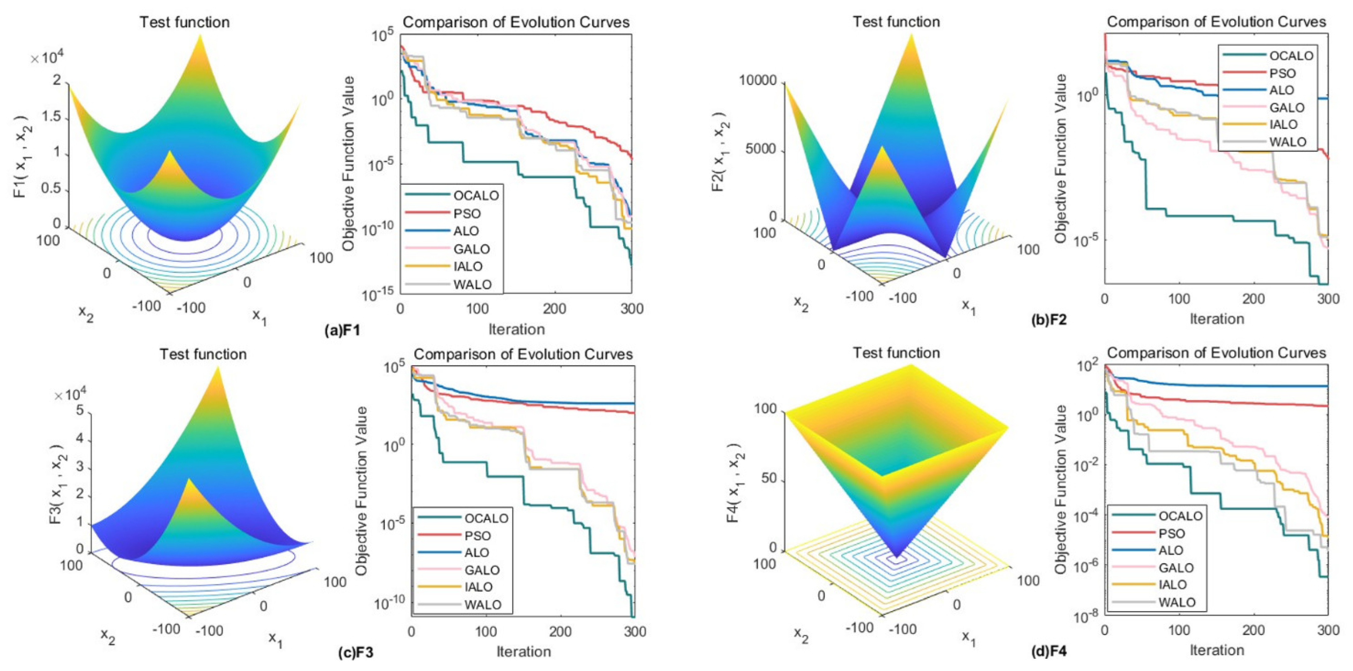
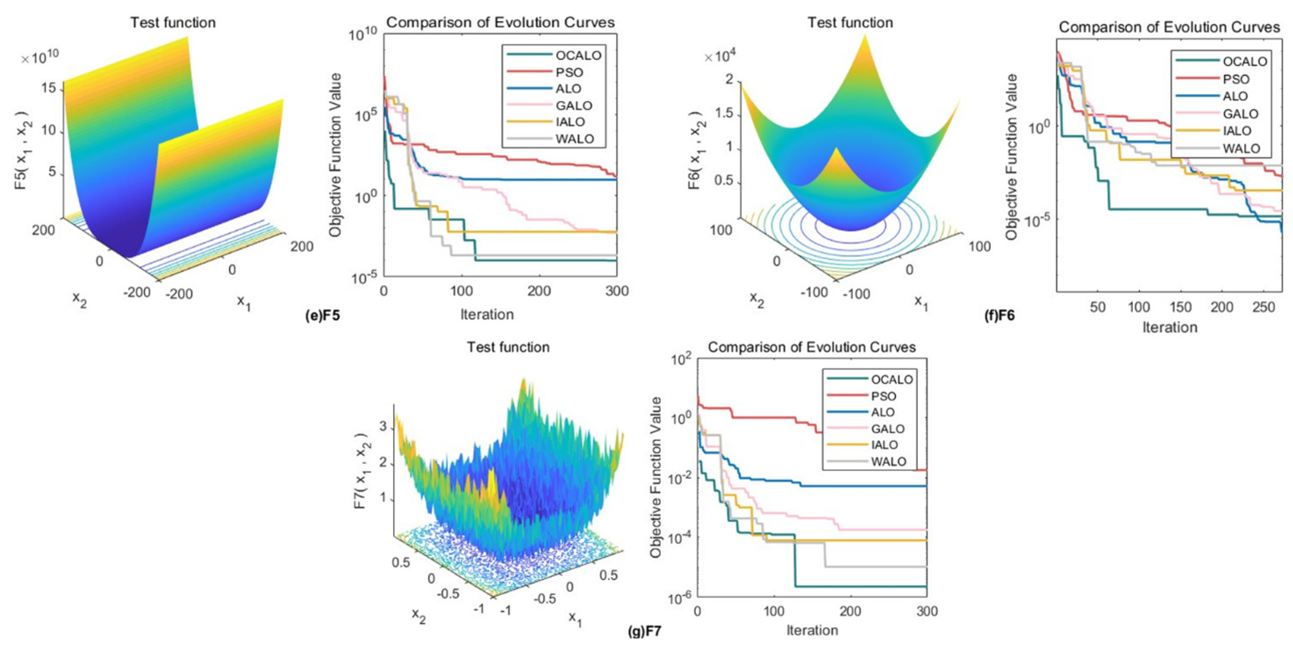
3.4. Comparison ofConvergence Curves ofFitness Values

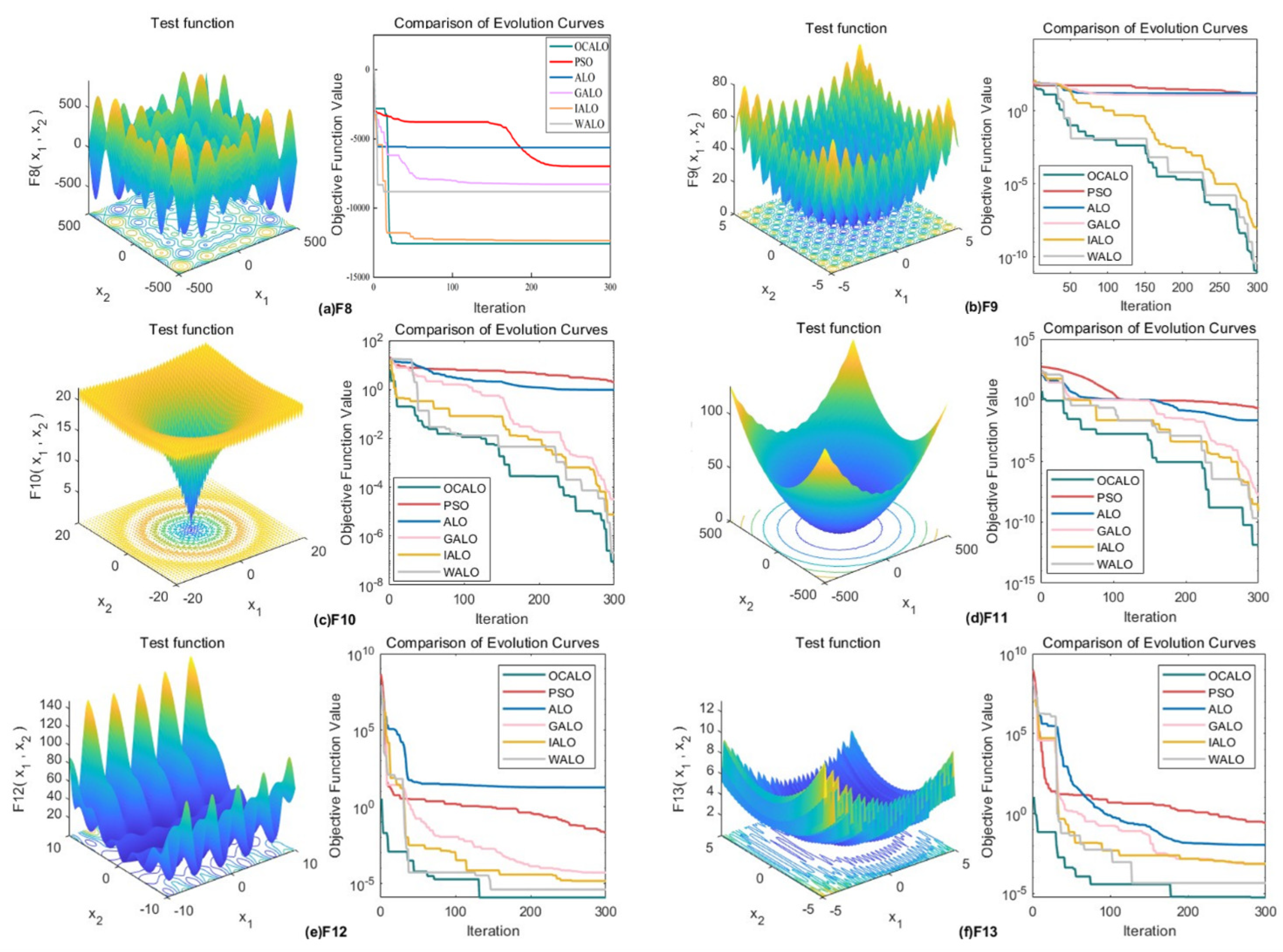
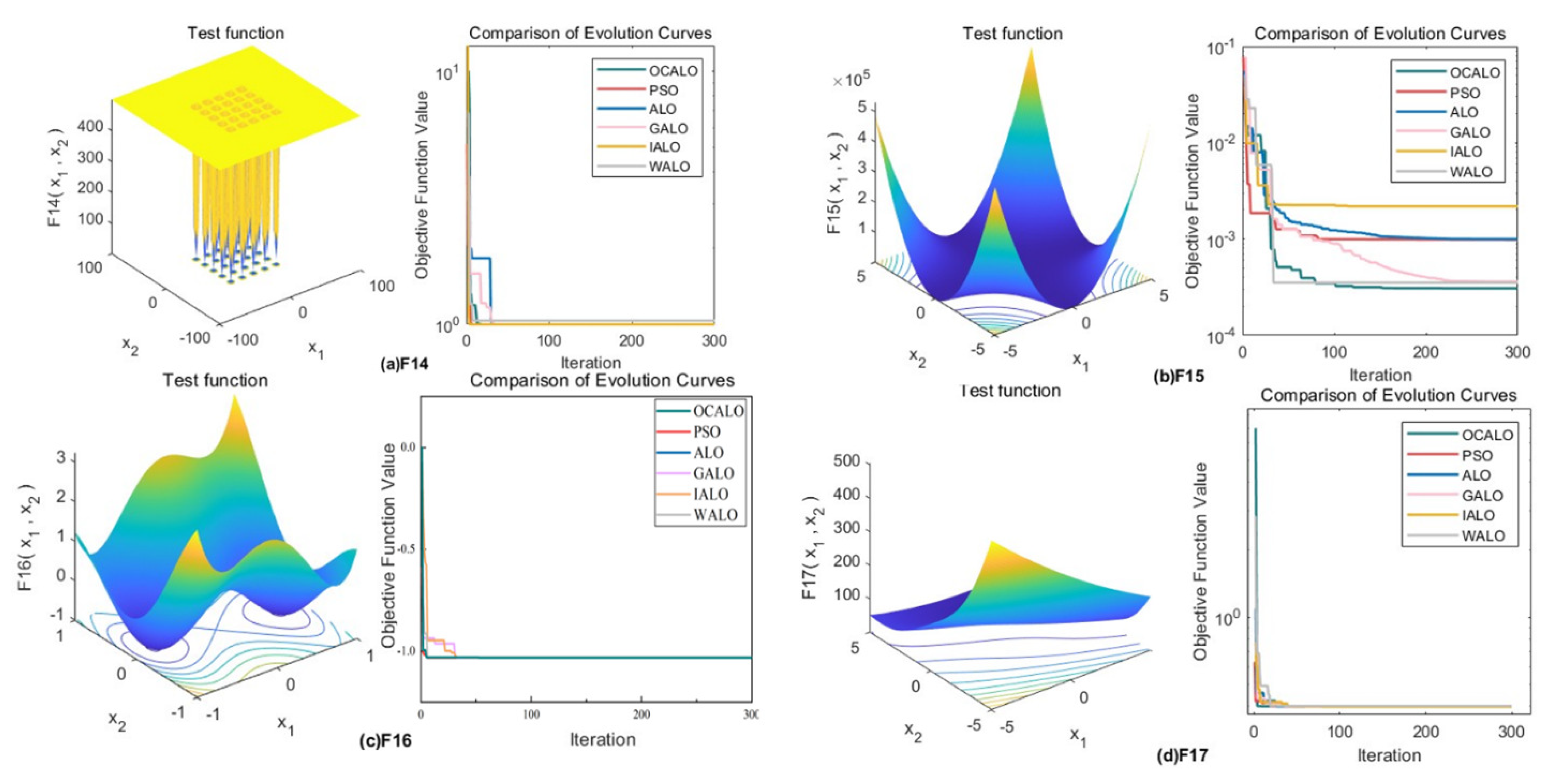
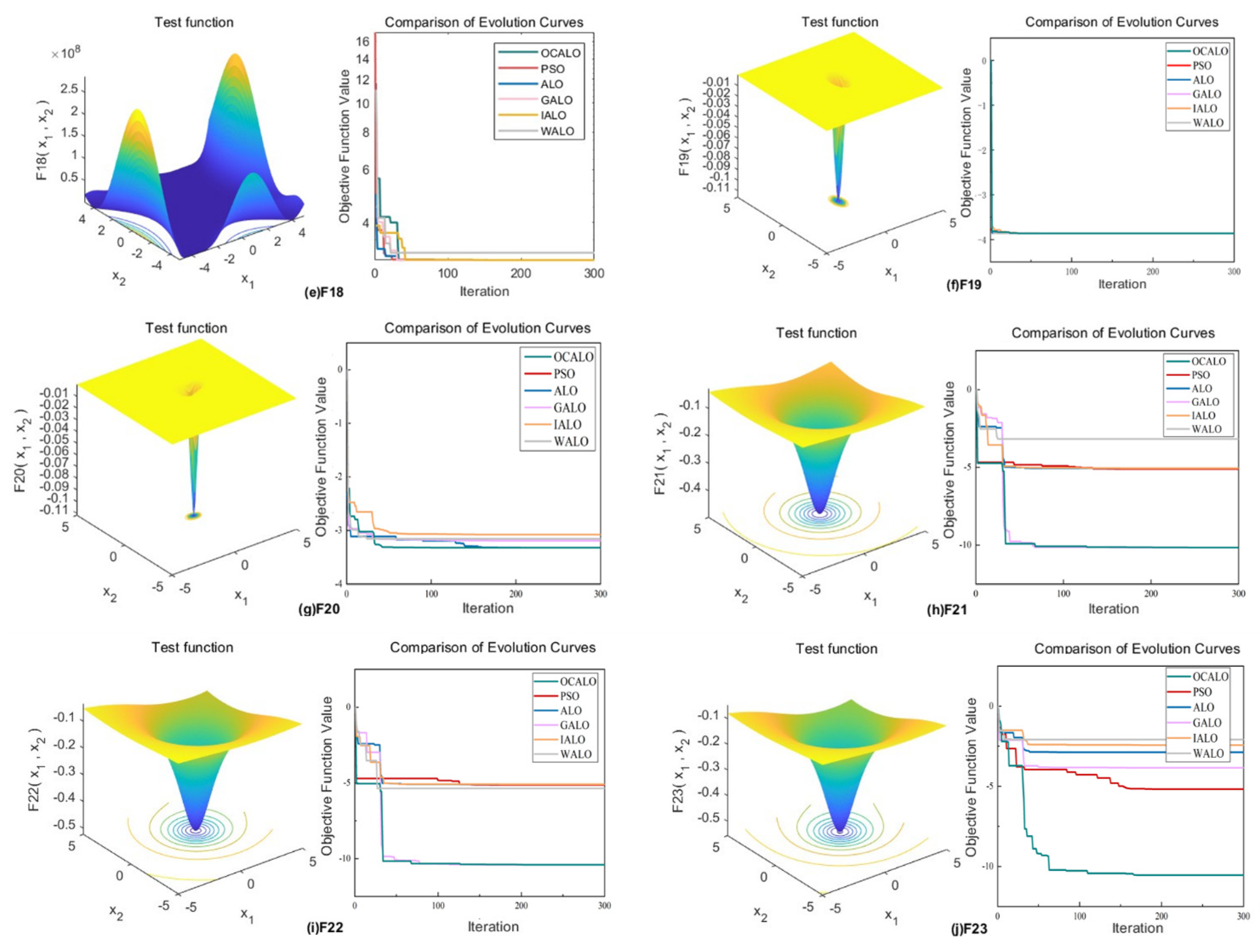
In order to reflect the dynamic convergence characteristics of OCALO and to further visually compare the convergence of the algorithms and the ability to jump out of the local optimum, the convergence curves of the 23 test functions are given for a total of 23 test functions under the five optimization algorithms, where the horizontal coordinates are the number of iterations and the vertical coordinates are the values of the fitness function. It is shown in Figure 3, Figure 4 and Figure 5.

In summary, it can be seen that OCALO has significantly improved the search ability for different types of benchmark functions, whether it is a high-dimensional single-peak function, high-dimensional multi-peak function, fixed-dimensional multi-peak function. At the same time, its fast convergence speed and short operation time can meet the demand for real-time algorithms and effectively avoid falling into local optimum while ensuring the search speed, thus proving the feasibility and superiority of OCALO.

4. Performance Analysis of High-speed 3D printing model for Temperature Control

4.1. High-speed 3D printing Model Identificatio

The 3D printing nozzle heating time versus temperature obtained after running for 500 seconds is shown in Table 7 for some of the data.The real-time temperature profile of the high-speed FDM 3D printing nozzle will have a small oscillating effect.

Considering that due to the modelling process of the 3D printing nozzle and its complexity, the transfer function of the first order inertial delay system is difficult to capture the complex dynamic behaviour of the nozzle, in order to conveniently analyse and control the dynamic response of the whole system, the form of the transfer function of the system is designed as a second order model as shown in Equation (14).

$$G\left(s\right)=\frac{k{\omega }^2{e}^{-\theta s}}{s^2+2\xi \omega s+{\omega }^2}$$

(14)

where k is system gain. $\omega$ is the Frequency. $\xi$ is the Damping Factor.$\theta$ is the Delay.

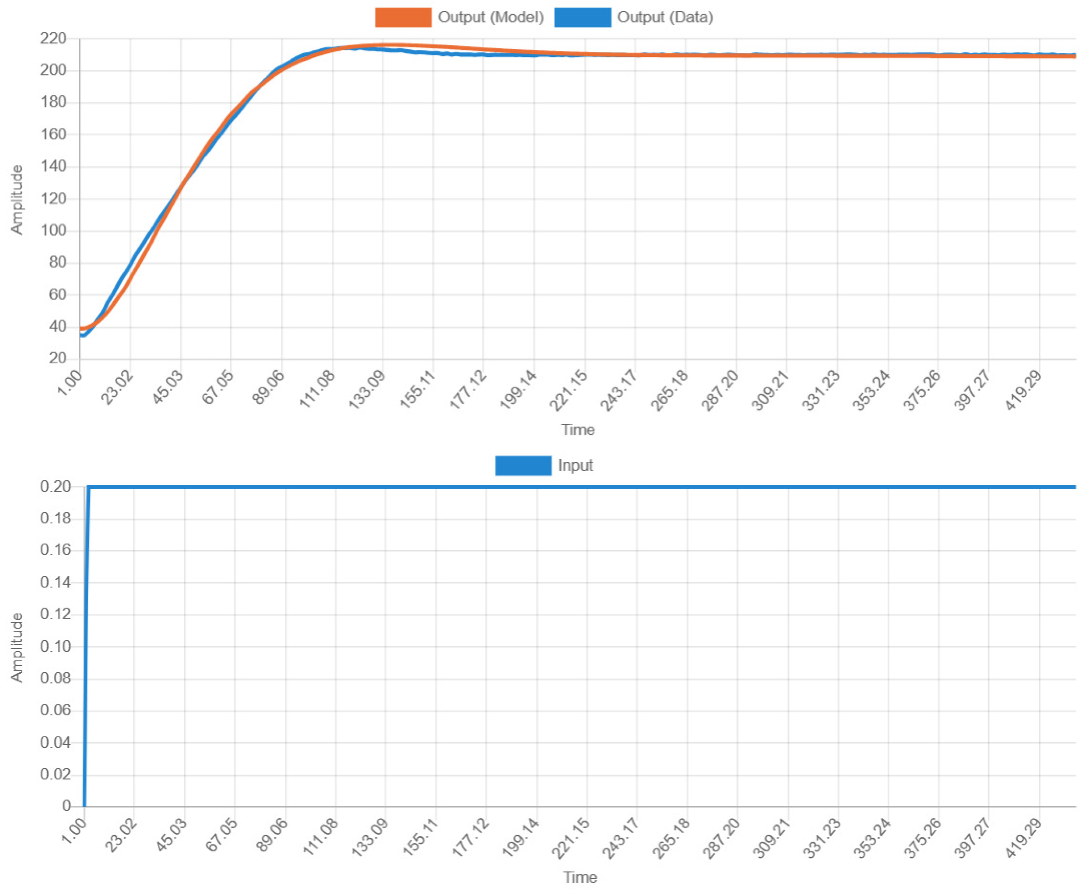
The values of the parameters were obtained by fitting the output curves as shown in Figure 7.

Based on the fitted response curve in Table 8, the process transfer function can be derived as Equation (15).Since the temperature system of 3D printing is a typical time delay system, in this paper, the time delay is set to 20.

$$G\left(s\right)=\frac{1.014}{s^2+0.05s+0.001}{e}^{-20s}$$

(15)

4.2. Controller Design

The quality of the parameters in the PID controller will greatly affect the quality of the controller. In this paper, we design an optimal PID controller based on the improved Ant-Lion optimization algorithm, with the aim of finding a set of optimal parameters in the solution space $K_p$, $K_d$,$K_i$, so that the system meets the control requirements and performs well. In designing the OCALO algorithm PID controller, the objective function should be set in accordance with the performance index of the control system and obtain satisfactory dynamic characteristics of the iterative process, and the evaluation function T is set as shown in Equation (16).

$$T={\int }_0^{\infty }\left(w_1\left|e\left(t\right)\right|+w_2{u}^2\left(t\right)\right)\mathrm{d}t$$

(16)

where $e\left(t\right)$is the error of the output value with respect to the input value. $u\left(t\right)$ is the control value of the control margin. $w_1$ is the weight value, which takes the value [0, 1], and usually $w_1$ = 0.999. $w_2$ is the weight value, which takes the value [0, 1], and usually $w_2$ = 0.001. In addition, a restriction is needed to prevent the overshooting, i.e., when the overshooting occurs, an additional overshooting term is introduced in the objective function, and the overshooting term $w_3\left|e\left(t\right)\right|$is introduced in the objective function Q as shown in Equation (17).

$$Q={\int }_0^{\infty }\left(w_1\left|e\left(t\right)\right|+w_2{u}^2\left(t\right)+w_3\left|e\left(t\right)\right|\right)\mathrm{d}t$$

(17)

Where $w_3$ is the weight value,$w_3$>>$w_1$,in general, $w_3$=100. The simulation model is built in simulink according to Equation (15). 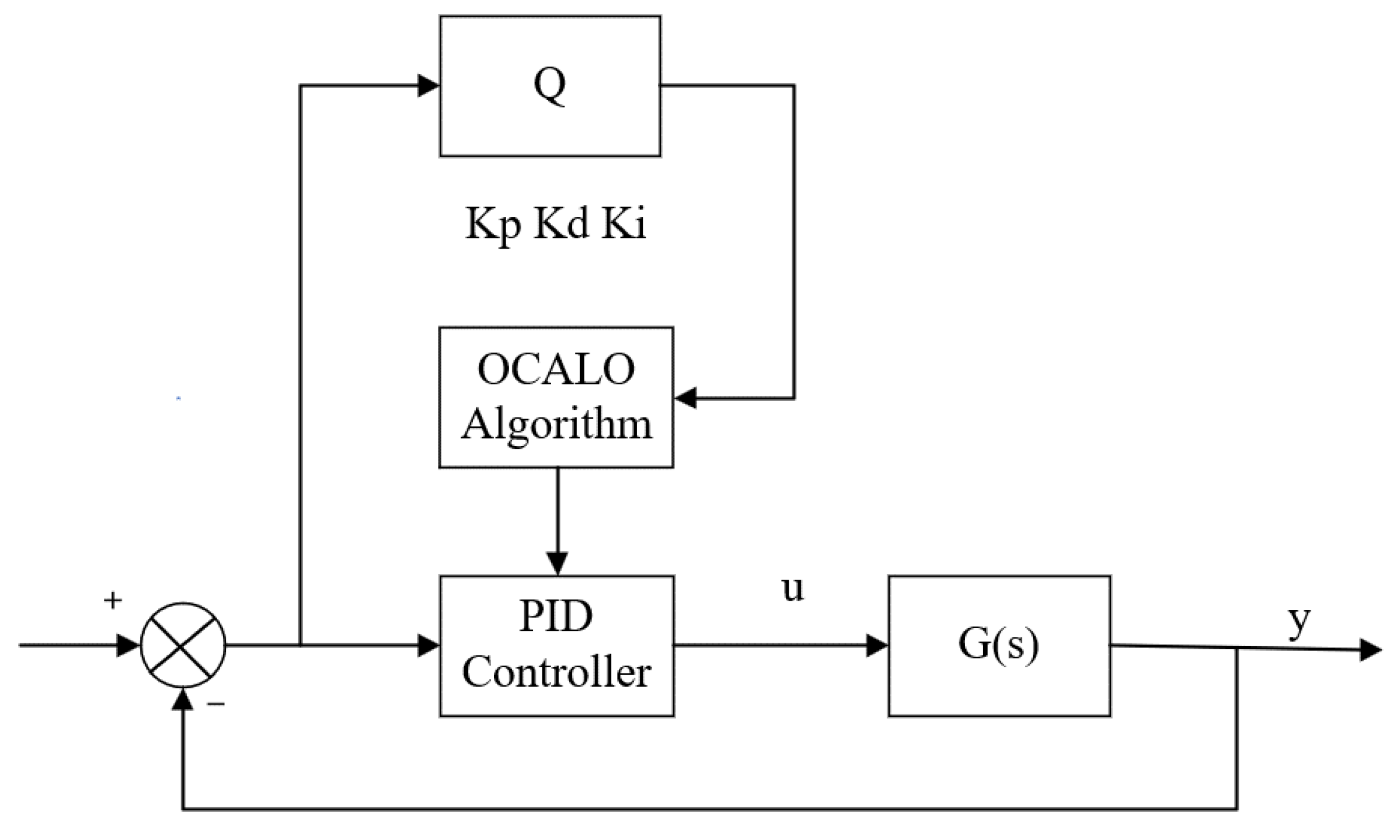The improved ant-lion optimization algorithm is used to design the PID controller, setting the parameter ranges $\mathrm{Kp},\mathrm{Kd},\mathrm{Ki}\in [0,100000]$, and Equation (17) as the fitness function, and the goal of the optimization search is to find a set of PID values that minimise the Q error by correcting the three parameters through the OCALO algorithm. The block diagram of the PID controller design based on the OCALO algorithm is shown in Figure 9.

Figure 8. Block diagram of optimized PID controller design based on OCALO algorithm.

Figure 8. Block diagram of optimized PID controller design based on OCALO algorithm.

4.3. System Simulation and Results Analysis

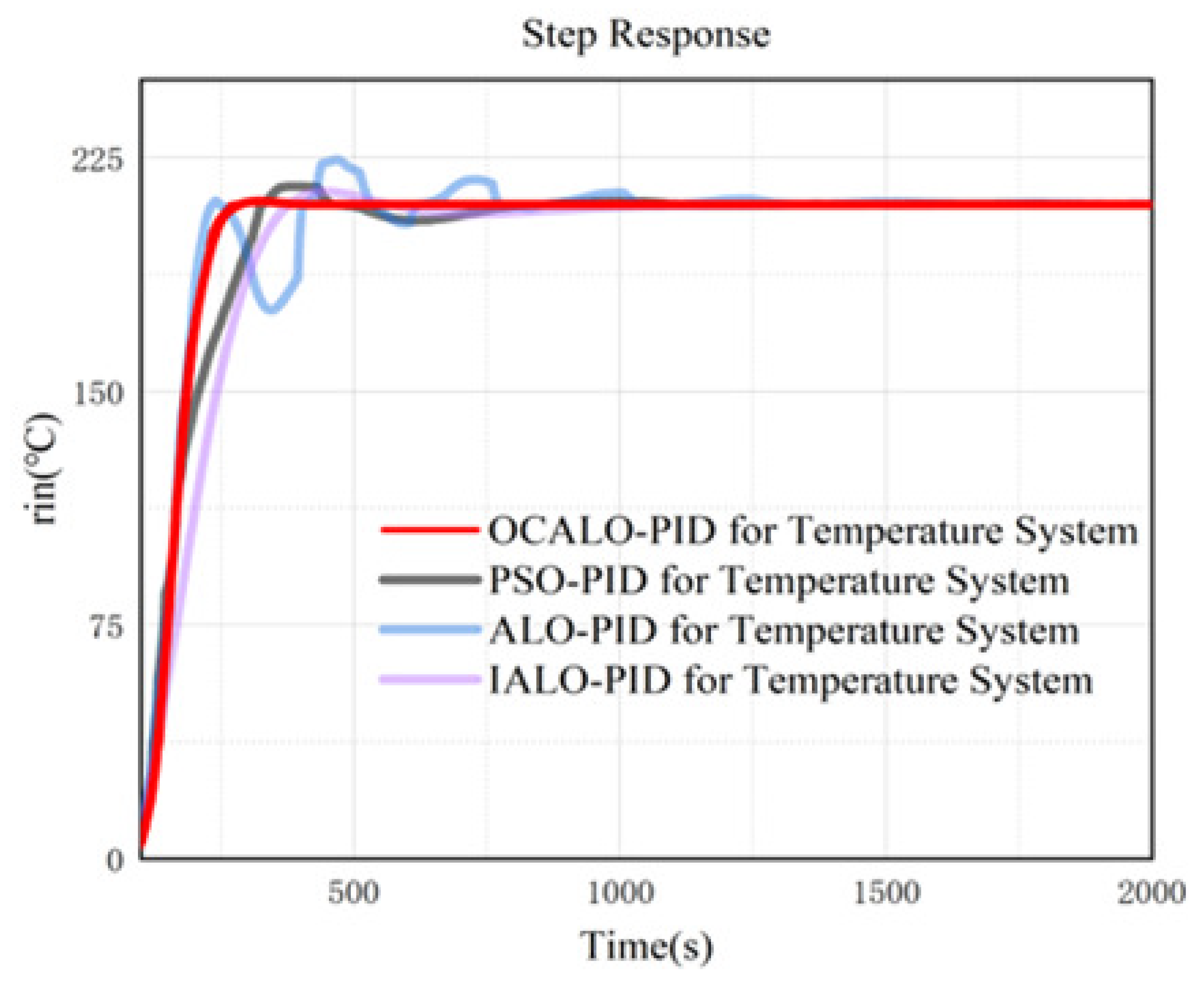
In this paper, only OCALO algorithm is listed with PSO algorithm, ALO algorithm and IALO algorithm, because WALO algorithm and GALO algorithm optimize the PID of the model temperature system with a very slow convergence speed, so they do not draw their curves on the graph. From Figure 9, it is easy to see that the OCALO algorithm has a faster response, the least amount of overshooting and the fastest response when it optimizes the PID of the temperature system.

Figure 9. Partial algorithmic PID controller for temperature systems.

Figure 9. Partial algorithmic PID controller for temperature systems.

According to Table 8, through the peak amplitude, peak time, rise time, Settling time four aspects of the analysis, OCALO algorithm peak amplitude is the smallest indicates that the system in the process of PID rectification compared to other algorithms overshoot the smallest amount of the system is the most stable; the peak time as well as the shortest rise time indicates that the process of PID rectification compared to other algorithms with the shortest response time, the fastest response time; stabilisation time compared to other algorithms is the shortest, so that can be to a certain extent to save the high-speed printing time costs.

Table 9. Simulation results of PID controller.

Variable	OCALO	PSO	ALO	IALO
Peak amplitude	1.59774	5.7589	14.3121	4.0686
Peak time	321.4505	385.3550	469.4281	451.4830
Rise time	272.0981	328.0076	407.3485	379.7559
Settling time	351.3188	860.1506	619.9532	1040.6734

Table 9. Simulation results of PID controller.

Variable	OCALO	PSO	ALO	IALO
Peak amplitude	1.59774	5.7589	14.3121	4.0686
Peak time	321.4505	385.3550	469.4281	451.4830
Rise time	272.0981	328.0076	407.3485	379.7559
Settling time	351.3188	860.1506	619.9532	1040.6734

The results show that OCALO has stronger robust search ability and the convergence speed can meet the real-time requirements. After establishing the FDM 3D printing nozzle model and determining its parameters, the OCALO-PID controller is designed, and through experimental simulation, the control curves of the OCALO-PID controller and the classical PID controller are compared under different control requirements, and it is concluded that the overall control performance of the OCALO-PID controller is better.

4.4. Interference Test

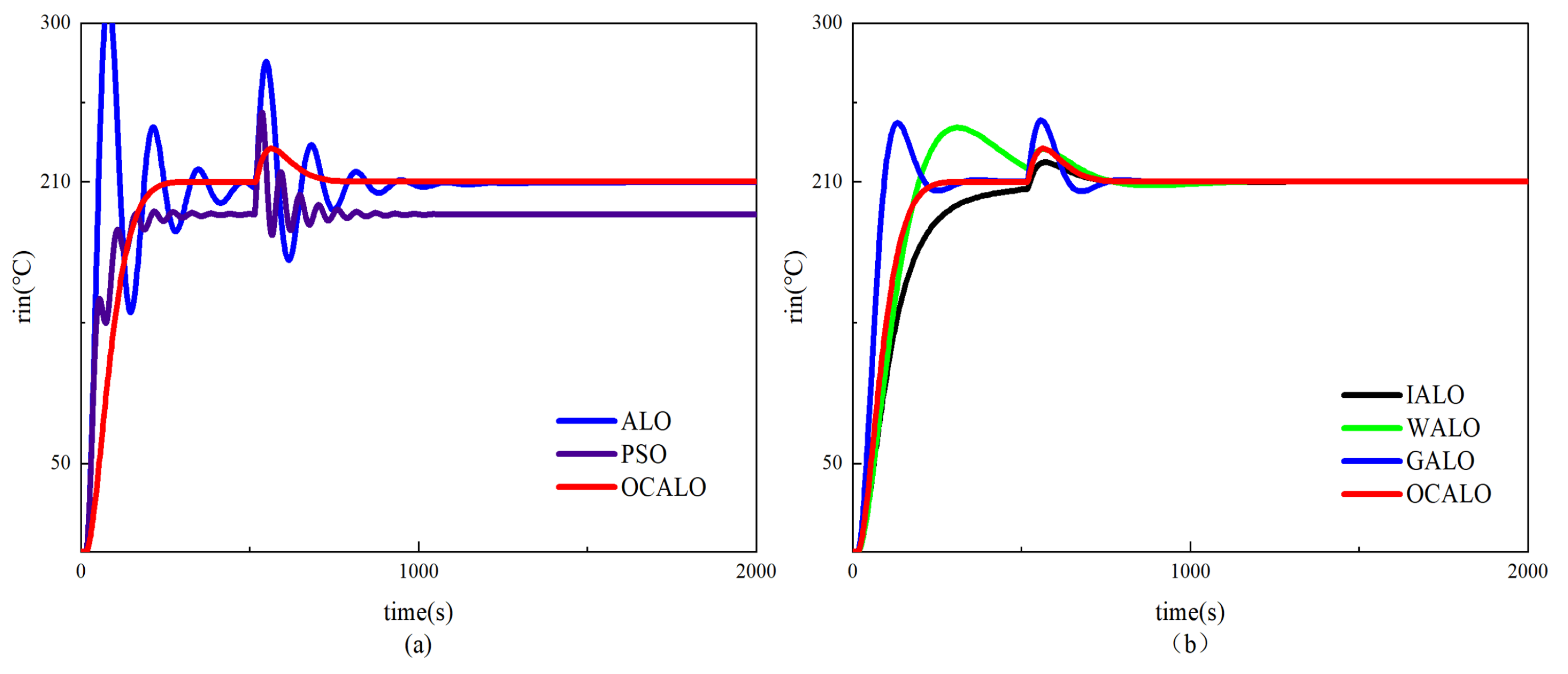
In performing high-speed 3D printing, the 3D printing nozzle in the face of a sharp turn of the printing task, due to the rapid rotation will cause the 3D printing nozzle vibration, so that has been stabilised at the target temperature of the 3D printing nozzle temperature system sudden load, resulting in temperature instability, affecting the quality of the print, this paper adds a perturbation at 520s, the OCALO algorithm with the classical algorithm(left) and the other improvements of the ALO algorithm(right) comparison for example Figure 11.

Analyzing Figure 10, compare the time for various controllers to recover to within 2error bars after being disturbed by a 0.1 step signal at 520 s, as shown in Table 10. Comparing the immunity of each algorithm in simulation.Determine the immunity to interference in the simulation by both the maximum peak value and the time required for recovery.

Figure 10. (a)Comparison of classical algorithms after sudden loading. (b) Comparison of Improved Algorithms after sudden loading.

Figure 10. (a)Comparison of classical algorithms after sudden loading. (b) Comparison of Improved Algorithms after sudden loading.

After the perturbation at 520 s, OCALO-PID has the smallest maximum peak, PSO-PID and ALO-PID have already experienced oscillatory phenomena, and all other algorithms have larger peaks than OCALO-PID. the amplitudes of PSO-PID and ALO-PID are still outside of the2 % error bars at 1000 s, and the shortest time used by OCALO-PID is 225.1 s , 22.4 s faster than GALO-PID, 19.1 s faster than IALO-PID, and 17.8 s faster than WALO-PID, and the difference in the recovery time is smaller compared to SSA-PID, but it is also 10.8 s faster, verifying that the OCALO-PID controllers are more resistant to disturbances than the other controllers.The OCALO-PID controller shows good performance in simulation, but it needs to be validated by applying it to an actual high-speed 3D printing temperature system.

5. Performance Analysis on Physical Platform Validation

5.1. Experiment platform construction

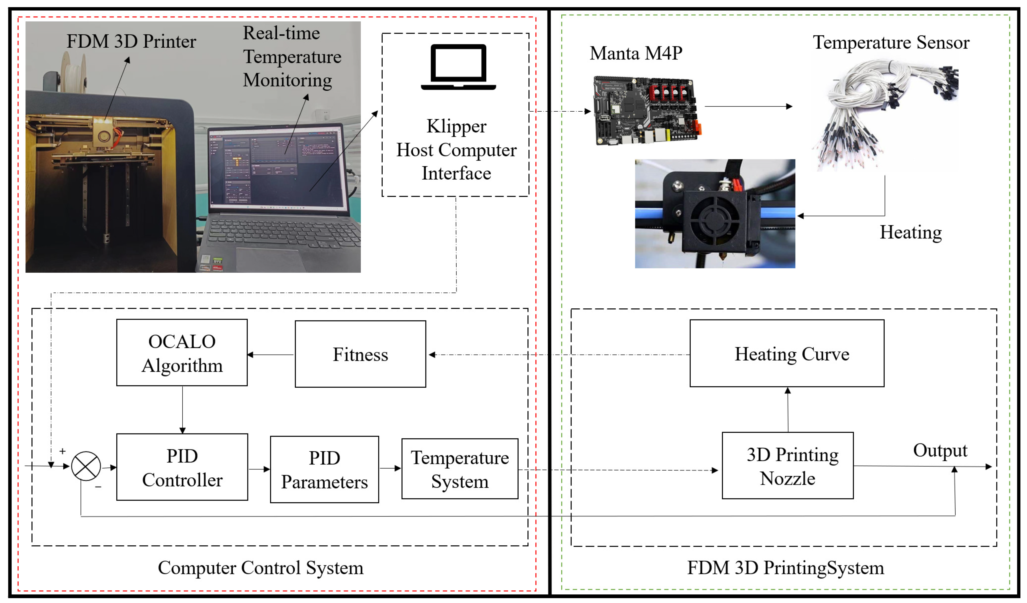
In order to verify the control effect of OCALO-PID controller on the temperature system of high-speed FDM 3D printing, this paper builds an experimental platform as in Figure 11, and the upper computer is the web-side interface based on Klipper firmware. The real-time temperature monitoring module of the Klipper firmware provides feedback on the heating and vibration cancellation of the FDM 3D printing nozzle.

Figure 11. Setting up the experimental environment.

Figure 11. Setting up the experimental environment.

5.2. Response and stabilisation experiments

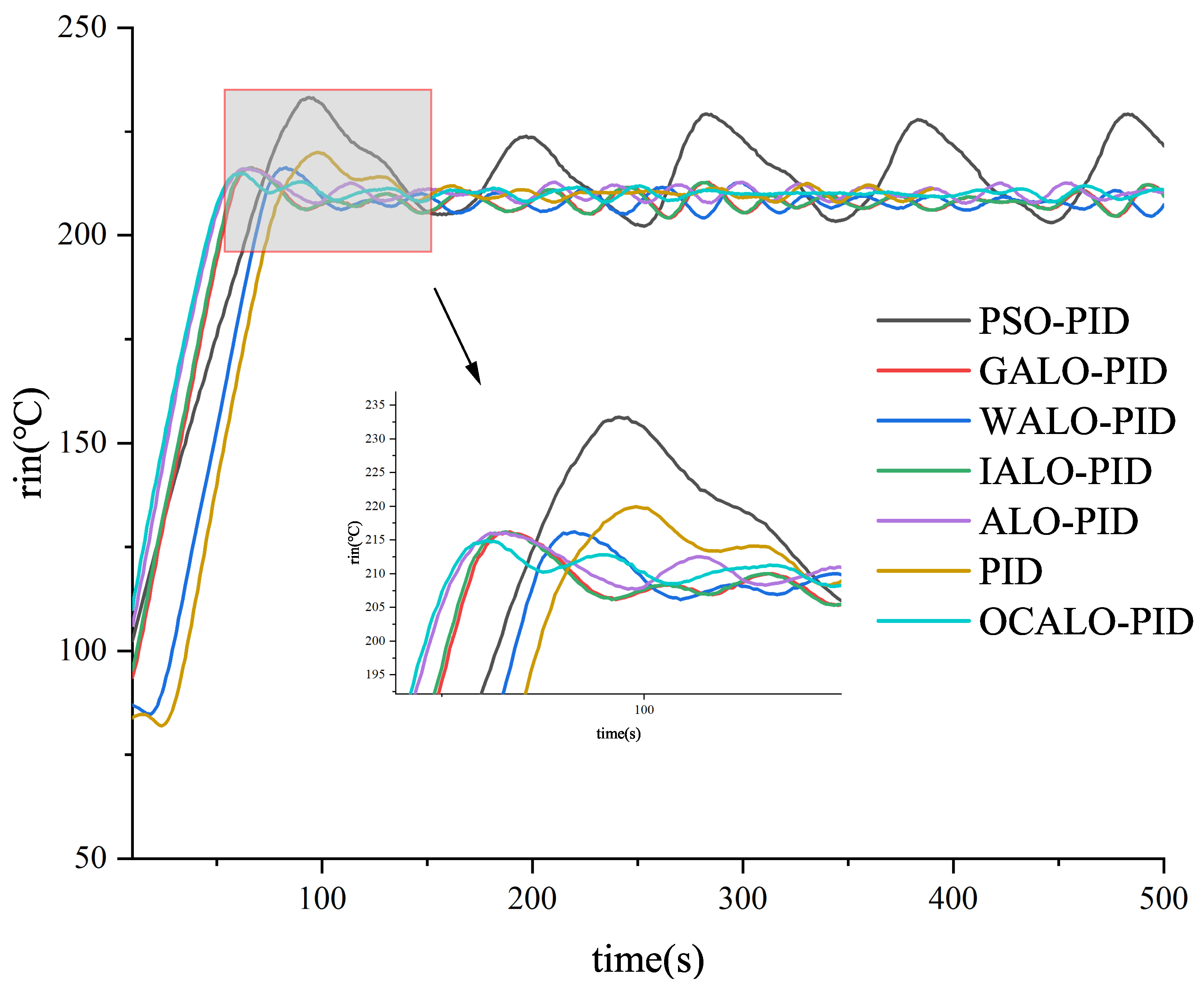
The desired temperature was set to 210 °C. The temperature of the 3D printing nozzle was controlled by PID parameters of the Klipper firmware. The temperature of the 3D printing was controlled by adding different algorithms. The temperature profile is shown in Figure 12.

As the actual 3D printing temperature will constantly jitter due to unavoidable reasons caused by the hardware, it is assumed in this paper that if there is a phase where the temperature jitter is less than 3°C, the temperature of the 3D printing printhead is considered stable.

Analysing Table 11, it can be seen that the OCALO algorithm not only achieves better responsiveness and robustness in the fitted simulation model, but also shows its good responsiveness and robustness in the actual high-speed 3D printing temperature system, and it can be seen that the OCALO algorithm achieves the fastest speed to reach the steady state and uses the least amount of actuality from Peak time and Stable time aspects.

5.3. Actual Interference Test

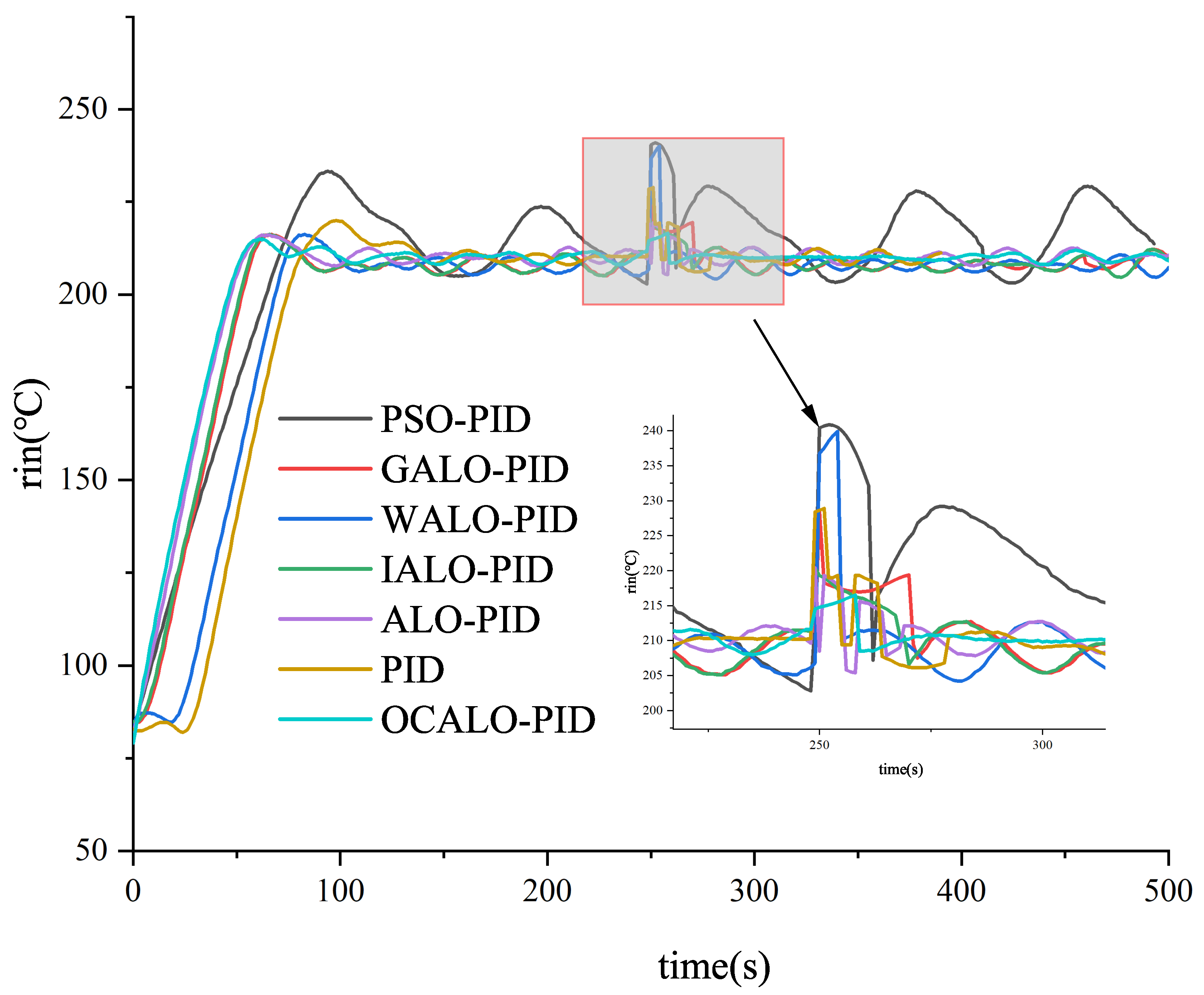
In real high-speed 3D printing application environments, different perturbations are often encountered,the cause of the perturbations may be due to human control requirements, or due to fast stepping movements, or may be indeterminate. Therefore, perturbation testing of algorithms is needed as a way to verify that the robustness of the algorithm meets the requirements. Perturbation of all algorithms.Add artificial perturbations in real environment 3D printing run 250 s. Figure 13 shows the perturbation test plot for all algorithms.

Table 12. Performance index.

Algorithm	Steady-State Error (◦C)	Recovery Time (s)
PSO-PID	30.4	-
GALO-PID	18.5	376
WALO-PID	26.7	369
IALO-PID	10.4	370
ALO-PID	9.3	352
PID	9.6	340
OCALO-PID	6.5	261

Table 12. Performance index.

Algorithm	Steady-State Error (◦C)	Recovery Time (s)
PSO-PID	30.4	-
GALO-PID	18.5	376
WALO-PID	26.7	369
IALO-PID	10.4	370
ALO-PID	9.3	352
PID	9.6	340
OCALO-PID	6.5	261

Through the perturbation test, the OCALO-PID controller restores the steady state after 261 s, which is 115 s, 108 s, 109 s, 91 s, 79 s, and 131.4 s less than PSO-PID and GALO-PID, respectively, The steady state value of the OCALO-PID controller is 216.5 °C, and the error between setpoint and 121 °C is only 6.5 °C. The recovery time is much shorter than that of the PSO-PID and GALO-PID. The steady-state value of the OCALO-PID controller is 216.5 °C, and the error between the setpoint and 121 °C is only 6.5 °C, which is 30.4 °C, 18.5 °C, 26.7 °C, 10.4 °C, 9.3 °C, and 9.6 °C lower than that of the PSO-PID and GALO-PID, respectively, The steady state errors of PSO-PID,WALO-PID, IALO-PID, ALO-PID and PID are smaller, respectively. Therefore, the OCALO-PID controller has excellent performance to meet the robustness of high-speed 3D printing.

6. Conclusions

This paper improves the ALO algorithm to solve the temperature control problem in high-speed 3D printing, which provides a model and algorithm reference for other similar temperature control systems. The main work of this paper is summarised as follows:

(1) A new Tent-Logistic-Cotangent composite chaotic mapping is proposed to improve the efficiency of population initialisation.The improved tent chaotic sequence is uniformly distributed between [0,1] with good traversal.

(2) Based on the traditional ALO algorithm, an algorithmic initialisation population method combining Tent-Logistic-Cotangent compositechaotic mapping and Elite Opposition-Based learning as well as an improved elitist formula are proposed to be applied to the algorithm.The improved ALO algorithm is placed in the same benchmark function test set with the other five algorithms to verify the superiority of the improved algorithm by comparing the mean, optimum, minimum, sample variance and the number of iterations.

(3)The improved algorithm is applied to a physical simulation platform based on Klipper firmware and compared with five other algorithms as well as the classical PID algorithm. Response experiments and anti-interference experiments are compared with other algorithms to verify that the improved algorithm has a clear response capability and stability.

In this study, a new Tent-Logistic-Cotangent chaotic mapping is used in the initialisation improvement of the algorithm, which improves the efficiency of population generation more effectively, but makes the algorithm relatively more complex and increases the difficulty of integration. Much of the main work in this paper has been to validate the feasibility of the algorithm, and the physical modelling process has been relatively crude, with further research allowing optimization of the control model to achieve the improvements. As we move towards 3D printing manufacturing, future research will be closer to practical needs, and future control systems for high-speed 3D printing will need to continually face difficult upgrades, so this paper’s single addition of a disturbance is slightly insufficient, and future research can improve the simplicity of the algorithm as well as increase its reliability in the actual 3D printing process.

References

- Peng Geng and Ji Zhao. Effects of extrusion speed and printing speed on the 3D printing stability of extruded PEEK filament. Journal of Manufacturing Processes, 2019, 37, 266–273. [CrossRef]
- Nazir A, Jeng J-Y. A high-speed additive manufacturing approach for achieving high printing speed and accuracy. Proceedings of the Institution of Mechanical Engineers 2020, 234, 2741–2749.
- X. Wu, X. Wang and G. He. A Fuzzy Self-tuning Temperature PID Control Algorithms for 3D Bio-printing Temperature Control System. 2020 Chinese Control And Decision Conference (CCDC); 2020; pp. 2846–2849.
- V. Schmidtke, M. Rüger and O. Stursberg. Model Predictive Control of PDEs for Temperature Control in 3D-Printing Processes. 2023 European Control Conference (ECC), 2023; pp. 1–6.
- Liu L H , Wei X K .Multiple Model Based Robust PID Control for Superheated Steam Temperature System[J]. Applied Mechanics and Materials, 2014, 494-495, 1266–1269. [CrossRef]
- Astrom K J , Hagglund T.The future of PID control[J]. Control Engineering Practice 2001, 9, 1163–1175. [CrossRef]
- Seyedali,Mirjalili,Pradeep,et al.Multi-objective ant lion optimizer: a multi-objective optimization algorithm for solving engineering problems[J]. Applied Intelligence 2016.
- K, Shankar and Lakshmanaprabu S.K.Optimal key based homomorphic encryption for color image security aid of ant lion optimization algorithm. International journal of engineering and technology 2022, 187.
- Kesarwani S , Verma R K.Ant Lion Optimizer (ALO) algorithm for machinability assessment during Milling of polymer composites modified by ze-ro-dimensional carbon nano onions (0D-CNOs)[J]. Measurement 2018, 7, 22.
- Li,Y.; Wu,Y.Gaussian mutation based ALO and its application in combinatorial optimization[J]. China Sciencepaper 2022, 17, 295–304.
- Wang,Y. ; Yu, H.; Ling D. ; et al.Optimization of BP for bearing fault diagnosis based on improved antlion algorithm[J/OL]. Computer Integrated Manufacturing Systems 2023, 1–21.
- Ji, J.; Wang, F.; Zhou, M.; Guo, R.; Ji, R.; Huang, H.; Zhang, J.; Nazir, M.S.; Peng, T.; Zhang, C.; et al. Evaluation Study on a Novel Structure CCHP System with a New Comprehensive Index Using Improved ALO Algorithm. Sustainability 2022, 14, 15419. [Google Scholar] [CrossRef]
- Mirjalili, Seyed Mohammad. The Ant Lion Optimizer. Adv. Eng. Softw. 2015, 83, 80–98. [CrossRef]
- Zhongyun Hua, Yicong Zhou, Hejiao Huang.Cosine-transform-based chaotic system for image encryption. Information Sciences 2019, 480, 403–419. [CrossRef]
- H. R. Tizhoosh.Opposition-Based Learning: A New Scheme for Machine Intelligence. International Conference on Computational Intelligence for Modelling, Control and Automation and International Conference on Intelligent Agents, 2005; pp. 695–701.
- Zhao, Jia and Li Lv.Shuffled frog-leaping algorithm using elite opposition-based learning. Int. J. Sens. 2019, Networks 16, 244–251.
- Yildiz, B.S., Pholdee, N., Bureerat, S. et al. Enhanced grasshopper optimization algorithm using elite opposition-based learning for solving real-world engineering problems. Engineering with Computers 2022, 38, 4207–4219. [CrossRef]
- Guo, J., Chen, C., Xiang, S. et al. A fast bilateral filtering algorithm based on rising cosine function. Neural Computing and Applications 2019, 1–12.
- Saeed, S.; Ong, H.C.; Sathasivam, S. Self-Adaptive Single Objective Hybrid Algorithm for Unconstrained and Constrained Test functions: An Application of Optimization Algorithm. Arab. J. Sci. Eng. 2019, 44, 3497–3513. [Google Scholar] [CrossRef]