Submitted:
25 January 2024
Posted:
26 January 2024
You are already at the latest version
Abstract
Keywords:
1. Introduction
2. Methodology
2.1. Development of the Approach
2.2. Deep Learning Models
2.2.1. ANN
2.2.2. Long Short-Term Memory
2.2.3. Informer
2.3. Model Application
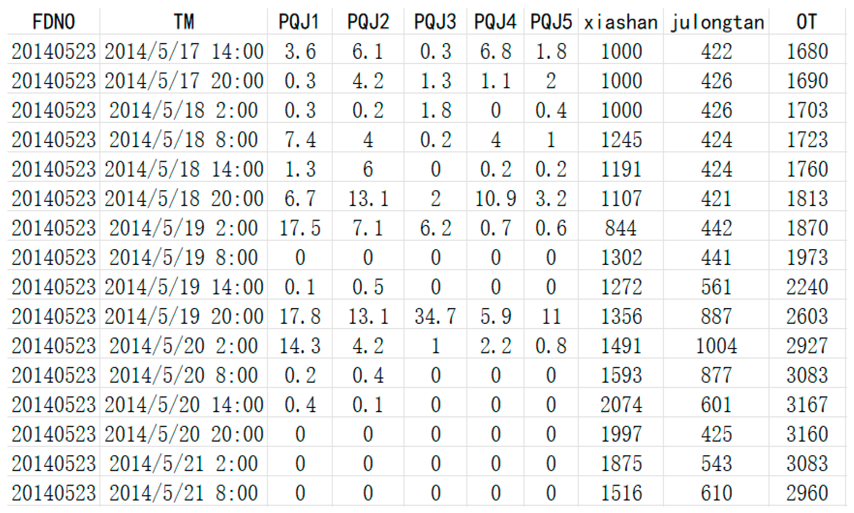
2.4. Model Performance Measures
3. Result
4. Discussion
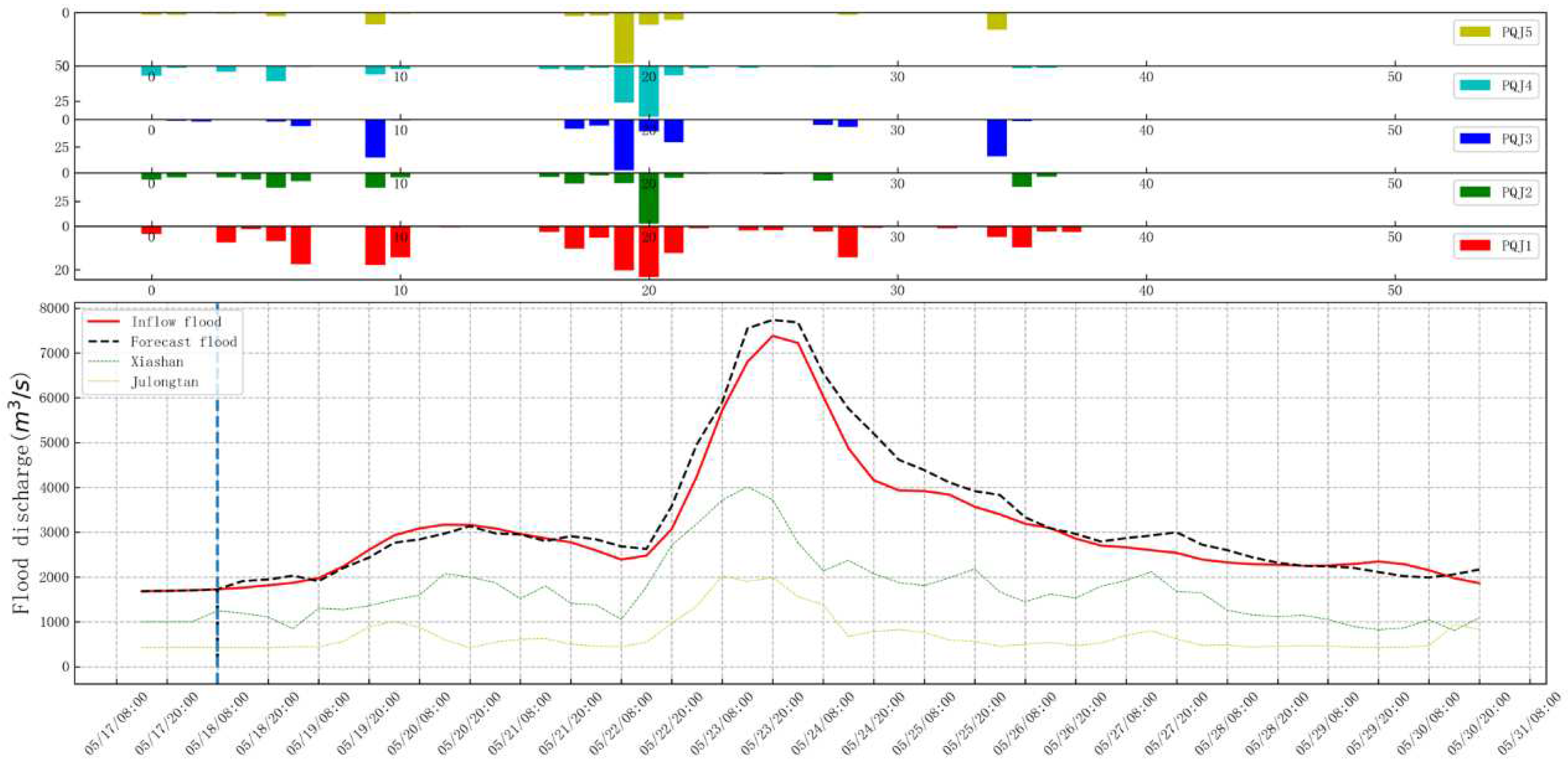
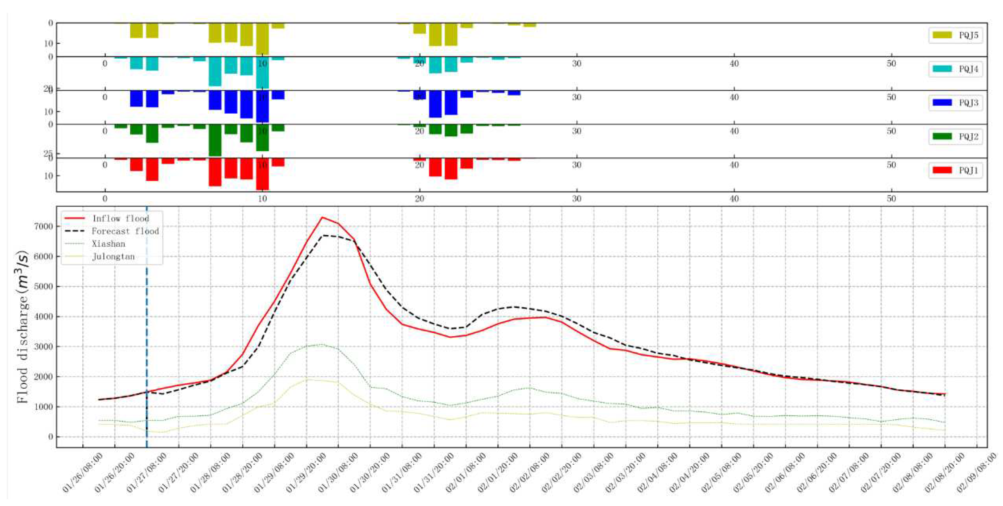
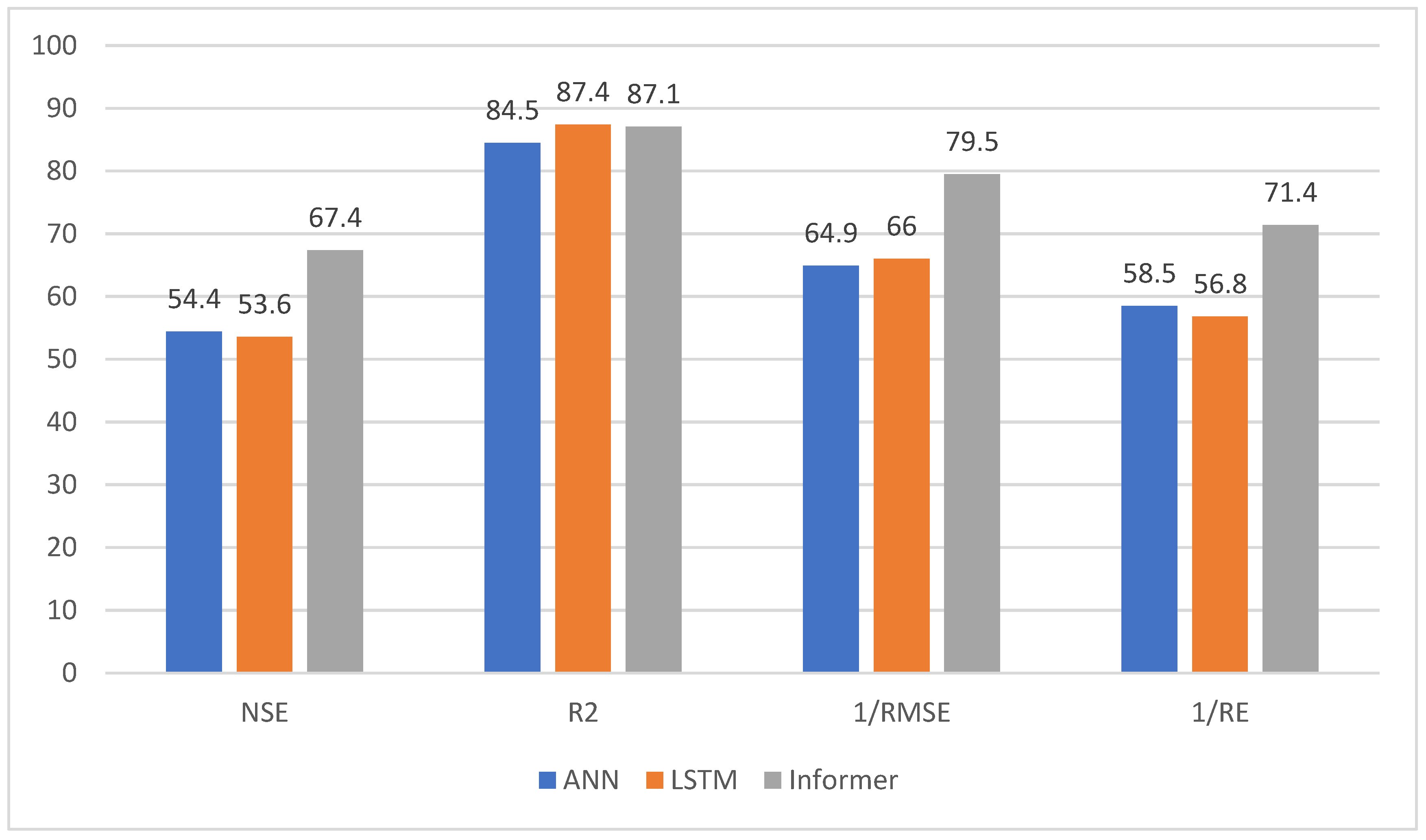
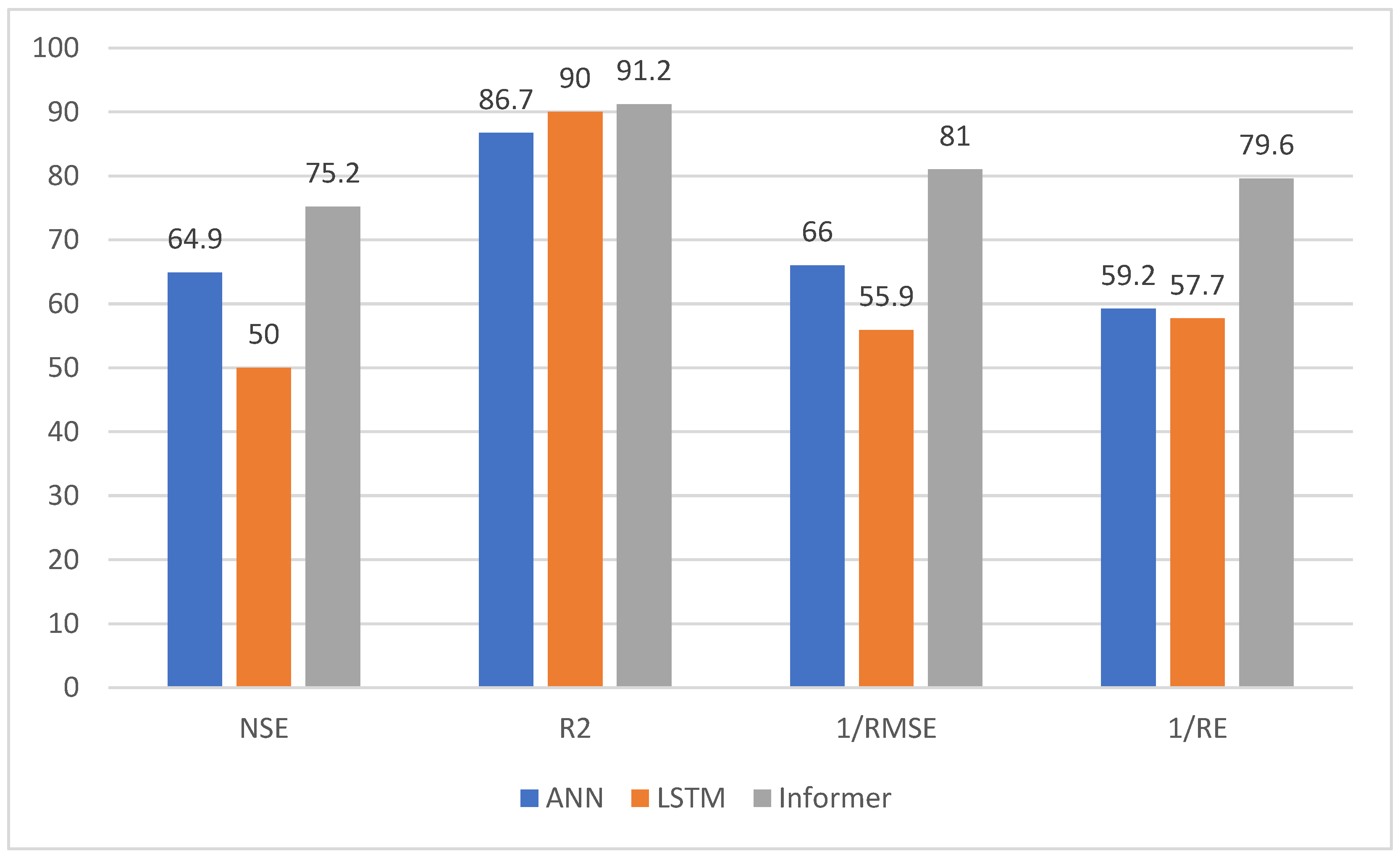
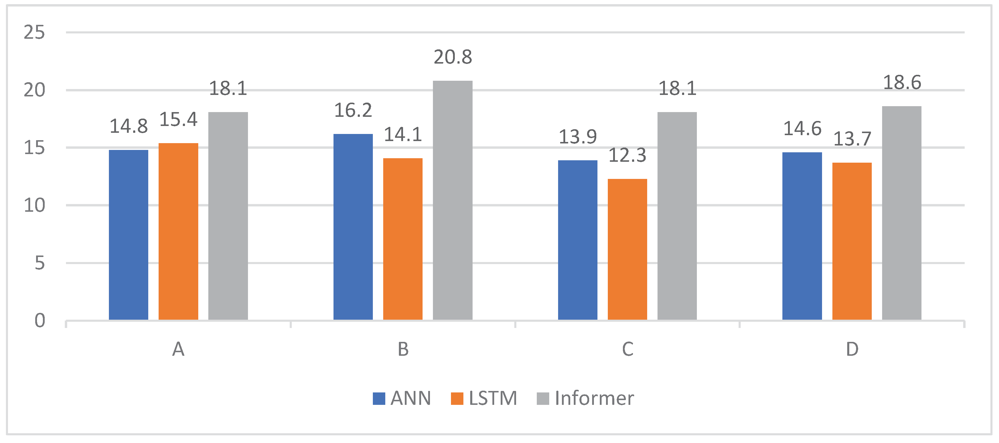
5. Conclusions
Acknowledgments
References
- Mlv, M.; Todini, E.; Libralon, A. A Bayesian decision approach to rainfall thresholds based flood warning. Hydrol. Earth Syst. Sci. Discuss. 2006, 2, 413–426. [Google Scholar] [CrossRef]
- Bartholmes, J.C.; Thielen, J.; Ramos, M.H.; Gentilini, S. The european flood alert system EFAS-Part 2: Statistical skill assessment of probabilistic and deterministic operational forecasts. Hydrol. Earth Syst. Sci. 2009, 13, 141–153. [Google Scholar] [CrossRef]
- Park, D.; Markus, M. Analysis of a changing hydrologic flood regime using the variable infiltration capacity model. J. Hydrol. 2014, 515, 267–280. [Google Scholar] [CrossRef]
- QIAO G C,YANG M X,LIU Q,et al. Monthly runoff forecast model of Danjiangkou Reservoir in autumn flood season based on PSO-SVRANN [J]. Water Conservancy and Hydropower Technology(Chinese and English),2021,52(4):69-78. [CrossRef]
- TAN Q F,WANG X,WANG H,et al. Application comparison of ANN, ANFIS and AR models in daily runoff time series prediction [J].South-to-North Water Transfer and Water Conservancy Science and Technology,2016,14(6):12-17+26. [CrossRef]
- Salas, J.D.; Markus, M.; Tokar, A.S. Streamflow forecasting based on artificial neural networks. Artif. Neural Netw. Hydrol. 2000, 36, 23–51. [Google Scholar] [CrossRef]
- Tokar, A.S.; Johnson, P.A. Rainfall-runoff modeling using artificial neural networks. J. Hydrol. Eng. 1999, 4, 232–239. [Google Scholar] [CrossRef]
- LIU H. Research on flood classification and prediction based on neu⁃ ral network and genetic algorithm [J]. Water Resources and Hydro⁃ power Technology,2020,51(8):31-38. [CrossRef]
- LI D Y,YAO Y,LIANG Z M,et al.Hydrological probability predic⁃ tion method based on variable decibel Bayesian depth learning [J/ OL].Water science progress:1-10. [CrossRef]
- XU Y,HU C,WU Q,et al.Research on particle swarm optimization in LSTM neural networks for rainfall-runoff simulation[J]. Journal of Hydrology,2022,608:127 553. [CrossRef]
- CUI Z,GUO S L,WANG J,et al.Flood forecasting research based on GR4J-LSTM hybrid model [J]. People′s Yangtze River,2022,53 (7):1-7. [CrossRef]
- OUYANG W Y,YE L,GU X Z,et al.Review of the progress of indepth study on hydrological forecasting II-Research progress and prospects [J].South-to-North Water Transfer and Water Conservan⁃ cy Technology (Chinese and English),2022,20(5):862-875.
- YIN H,WANG F,ZHANG X,et al.Rainfall-runoff modeling using long short-term memory based step-sequence framework[J].Journal of Hydrology,2022,610:127 901. [CrossRef]
- LI B,TIAN F Q,LI Y K,et al. Deep-learning hydrological model in⁃ tegrating temporal and spatial characteristics of meteorological ele⁃ ments [J].Progress in Water Science,2022,33(6):904-913. [CrossRef]
- VASWANI A,SHAZEER N,PARMAR N,et al. Attention is all you need[J].Neural Information Processing Systems,2017,5998:6 008.
- SCHWALLER P, LAINO T,GAUDIN T,et al.Molecular transform⁃ er:A model for uncertainty-calibrated chemical reaction prediction. [J].ACS Central Science,2019,5(9):1 572-1 583. [CrossRef]
- WANG W,XIE E,LI X,et al. Pyramid vision transformer: A versa⁃ tile backbone for dense prediction without convolutions[C]// 2021 IEEE/CVF International Conference on Computer Vision (ICCV), 2021:548-558.
- ZHOU C H,LIN P Q. Traffic volume prediction method based on multi-channel transformer [J]. Computer Application Research, 2023,40(2):435-439. [CrossRef]
- DONG J F, WAN X, WANG Y,et al. Short-term power load fore⁃ casting based on XGB-Transformer model [J]. Power Information and Communication Technology,2023,21(1):9-18. [CrossRef]
- LI S,JIN X,XUAN Y,et al.Enhancing the locality and breaking the memory bottleneck of transformer on time series forecasting[J]. Neural Information Processing Systems,2019,32. [21] LIU C,LIU D,MU L. Improved transformer model for enhanced monthly streamflow predictions of the Yangtze River[J]. IEEE Access,2022,10:58 240-58 253.
- ZHOU H Y, ZHANG S H, PENG J Q, et al. Informer: beyond efficient transformer for long sequence time- series forecasting[C]//Proceedings of the 35th AAAI Conference on Artificial Intelligence, the 33rd Conference on Innovative Applications of Artificial Intelligence, the 11th Symposium on Educational Advances in Artificial Intelligence, Feb 2-9, 2021. Menlo Park: AAAI, 2021: 11106-11115. [CrossRef]
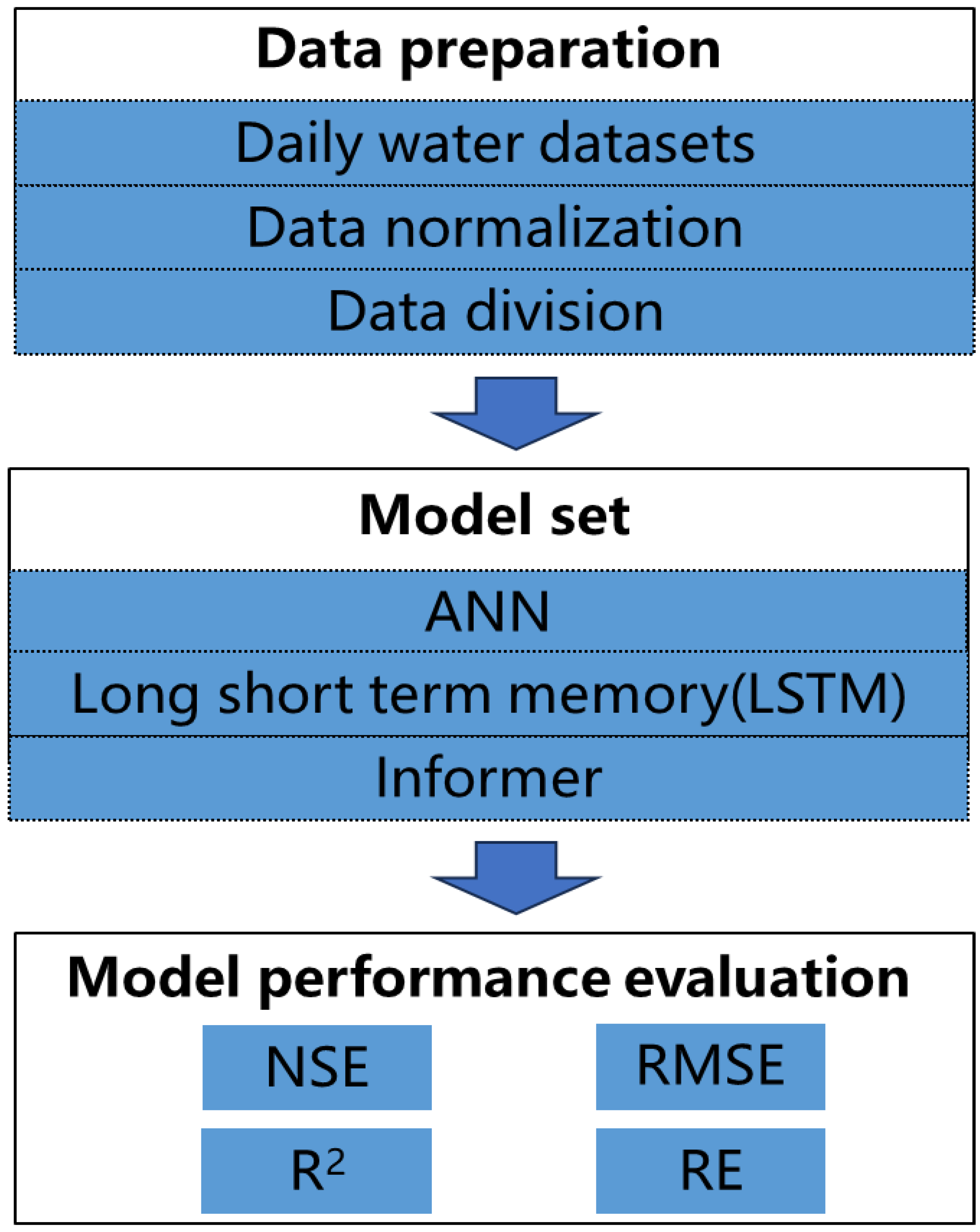
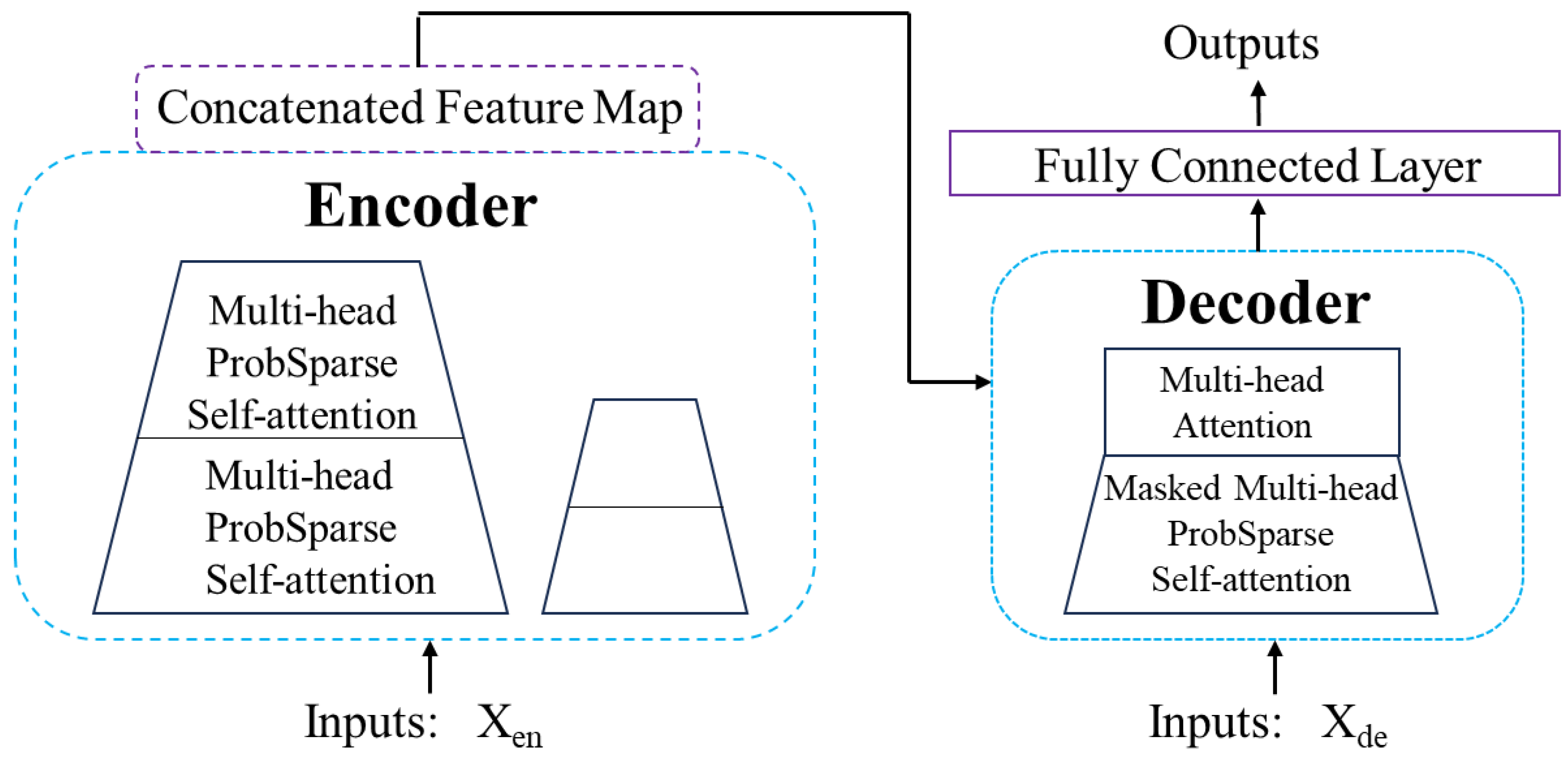
| Accuracy metrics | Loss | Seq len | ANN | LSTM | Informer |
|---|---|---|---|---|---|
| NSE | MAE | 4 | 0.487 | 0.407 | 0.675 |
| 5 | 0.492 | 0.500 | 0.639 | ||
| 6 | 0.416 | 0.436 | 0.522 | ||
| MSE | 4 | 0.628 | 0.711 | 0.746 | |
| 5 | 0.476 | 0.473 | 0.643 | ||
| 6 | 0.494 | 0.304 | 0.665 | ||
| Huber | 4 | 0.596 | 0.610 | 0.710 | |
| 5 | 0.641 | 0.665 | 0.719 | ||
| 6 | 0.672 | 0.715 | 0.744 | ||
| R2 | MAE | 4 | 0.832 | 0.878 | 0.859 |
| 5 | 0.836 | 0.882 | 0.851 | ||
| 6 | 0.842 | 0.833 | 0.855 | ||
| MSE | 4 | 0.847 | 0.895 | 0.873 | |
| 5 | 0.859 | 0.898 | 0.874 | ||
| 6 | 0.827 | 0.883 | 0.889 | ||
| Huber | 4 | 0.857 | 0.832 | 0.858 | |
| 5 | 0.842 | 0.877 | 0.884 | ||
| 6 | 0.859 | 0.886 | 0.893 | ||
| RMSE | MAE | 4 | 754 | 782 | 615 |
| 5 | 794 | 788 | 680 | ||
| 6 | 905 | 993 | 790 | ||
| MSE | 4 | 723 | 591 | 571 | |
| 5 | 755 | 789 | 665 | ||
| 6 | 822 | 936 | 602 | ||
| Huber | 4 | 789 | 704 | 590 | |
| 5 | 689 | 640 | 574 | ||
| 6 | 707 | 603 | 576 | ||
| RE(%) | MAE | 4 | 15.3 | 18.8 | 12.5 |
| 5 | 17.9 | 17.2 | 13.4 | ||
| 6 | 21.1 | 20.9 | 19.5 | ||
| MSE | 4 | 14.4 | 16.5 | 11.4 | |
| 5 | 18.5 | 16.9 | 16.9 | ||
| 6 | 16.6 | 20.1 | 14.3 | ||
| Huber | 4 | 16.1 | 17.2 | 11.7 | |
| 5 | 17.5 | 15.9 | 13.5 | ||
| 6 | 16.2 | 14.8 | 12.5 |
| Accuracy metrics | Loss | Seq len | ANN | LSTM | Informer |
|---|---|---|---|---|---|
| NSE | MAE | 4 | 0.689 | 0.672 | 0.822 |
| 5 | 0.652 | 0.566 | 0.743 | ||
| 6 | 0.656 | 0.594 | 0.684 | ||
| MSE | 4 | 0.674 | 0.734 | 0.775 | |
| 5 | 0.628 | 0.473 | 0.765 | ||
| 6 | 0.632 | 0.587 | 0.705 | ||
| Huber | 4 | 0.666 | 0.743 | 0.753 | |
| 5 | 0.612 | 0.747 | 0.792 | ||
| 6 | 0.636 | 0.736 | 0.757 | ||
| R2 | MAE | 4 | 0.885 | 0.887 | 0.923 |
| 5 | 0.842 | 0.910 | 0.898 | ||
| 6 | 0.866 | 0.874 | 0.912 | ||
| MSE | 4 | 0.863 | 0.910 | 0.916 | |
| 5 | 0.892 | 0.907 | 0.915 | ||
| 6 | 0.832 | 0.902 | 0.899 | ||
| Huber | 4 | 0.869 | 0.909 | 0.917 | |
| 5 | 0.886 | 0.910 | 0.915 | ||
| 6 | 0.885 | 0.905 | 0.906 | ||
| RMSE | MAE | 4 | 575 | 560 | 449 |
| 5 | 597 | 662 | 513 | ||
| 6 | 612 | 604 | 540 | ||
| MSE | 4 | 655 | 591 | 473 | |
| 5 | 667 | 789 | 479 | ||
| 6 | 692 | 655 | 512 | ||
| Huber | 4 | 753 | 521 | 512 | |
| 5 | 711 | 507 | 470 | ||
| 6 | 759 | 517 | 497 | ||
| RE(%) | MAE | 4 | 16.6 | 12.6 | 9.9 |
| 5 | 17.5 | 16.2 | 10.2 | ||
| 6 | 17.1 | 13.4 | 12.2 | ||
| MSE | 4 | 15.9 | 16.5 | 11.3 | |
| 5 | 16.1 | 16.9 | 11.4 | ||
| 6 | 17.5 | 15.8 | 11.2 | ||
| Huber | 4 | 17.5 | 11.9 | 14.4 | |
| 5 | 17.7 | 11.8 | 10.7 | ||
| 6 | 14.6 | 12.0 | 10.5 |
| Accuracy metrics | Loss | Seq len | ANN | LSTM | Informer |
|---|---|---|---|---|---|
| flood peak difference values less than 15% | MAE | 4 | 18 | 23 | 19 |
| 5 | 15 | 18 | 15 | ||
| 6 | 17 | 17 | 24 | ||
| MSE | 4 | 14 | 15 | 17 | |
| 5 | 14 | 13 | 17 | ||
| 6 | 15 | 12 | 21 | ||
| Huber | 4 | 13 | 15 | 13 | |
| 5 | 12 | 13 | 16 | ||
| 6 | 15 | 13 | 21 | ||
| flood peak difference less than 15% | MAE | 4 | 19 | 17 | 23 |
| 5 | 19 | 17 | 22 | ||
| 6 | 17 | 14 | 20 | ||
| MSE | 4 | 19 | 15 | 22 | |
| 5 | 15 | 12 | 21 | ||
| 6 | 19 | 12 | 21 | ||
| Huber | 4 | 14 | 14 | 16 | |
| 5 | 11 | 11 | 21 | ||
| 6 | 13 | 15 | 21 | ||
| NSE more than 0.8 | MAE | 4 | 14 | 14 | 18 |
| 5 | 15 | 16 | 17 | ||
| 6 | 16 | 13 | 19 | ||
| MSE | 4 | 14 | 11 | 18 | |
| 5 | 13 | 8 | 18 | ||
| 6 | 14 | 12 | 18 | ||
| Huber | 4 | 15 | 15 | 16 | |
| 5 | 13 | 10 | 19 | ||
| 6 | 11 | 12 | 20 | ||
| max flood peak gap (%) | MAE | 4 | 34.5 | 38.3 | 30.7 |
| 5 | 36.7 | 27.4 | 31.5 | ||
| 6 | 35.1 | 33.8 | 30.4 | ||
| MSE | 4 | 47.3 | 57.2 | 35.1 | |
| 5 | 39.4 | 36.3 | 35.1 | ||
| 6 | 42.1 | 49.2 | 32.7 | ||
| Huber | 4 | 49.7 | 61.0 | 37.7 | |
| 5 | 42.4 | 45.3 | 29.7 | ||
| 6 | 43.8 | 45.6 | 27.4 |
Disclaimer/Publisher’s Note: The statements, opinions and data contained in all publications are solely those of the individual author(s) and contributor(s) and not of MDPI and/or the editor(s). MDPI and/or the editor(s) disclaim responsibility for any injury to people or property resulting from any ideas, methods, instructions or products referred to in the content. |
© 2024 by the authors. Licensee MDPI, Basel, Switzerland. This article is an open access article distributed under the terms and conditions of the Creative Commons Attribution (CC BY) license (http://creativecommons.org/licenses/by/4.0/).


