Block Kinematic Wave, A Novel Rainfall-Runoff Model For Small Urban Catchments

Preprint

Article

Block Kinematic Wave, A Novel Rainfall-Runoff Model For Small Urban Catchments

Altmetrics

Downloads

Views

Comments

This version is not peer-reviewed

Submitted:

26 January 2024

Posted:

26 January 2024

You are already at the latest version

Alerts

Abstract

BKW is a highly efficient Storage Function-type rainfall-runoff model that utilizes the steady-state storage (S) and outflow (Q) of a catchment at different rainfall intensities as the S-Q relation of the catchment. For the inundation nowcasting of urban areas under high-intensity, short-duration rainfall, a Storage Function-type model is a judicious choice. However, S-Q hysteresis exists in the catchment S-Q relation, and BKW is unable to exhibit hysteresis due to assuming that the S-Q relation of a catchment is a nonlinear relation. The S-Q hysteresis can influence the outflow estimation of BKW, reducing the model's accuracy. Through the evaluation of analytical solutions, we found that the change in rainfall intensity dominates the S-Q relation of a catchment. The S-Q relation during a rainfall event is a dynamic process rather than a monotonic nonlinear relation. By applying the dynamic S-Q relation in BKW, we improved BKW to become a highly efficient and accurate rainfall-runoff model for small urban catchments.

Keywords:

Subject: Engineering - Civil Engineering

1. Introduction

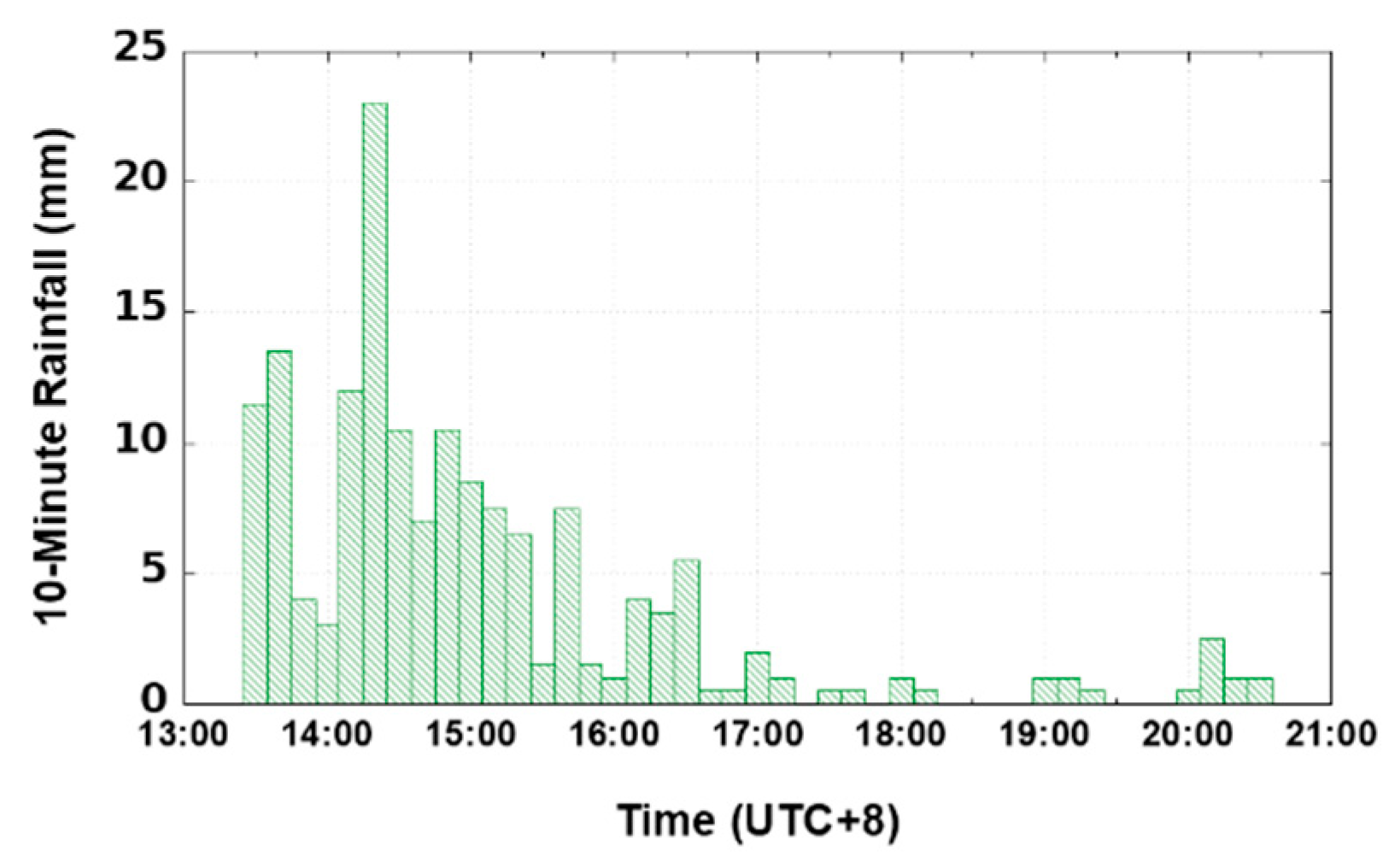
The occurrence of afternoon thunderstorm rain represents a meteorological phenomenon that is particularly prevalent during the summer months in Taiwan, spanning from May to September. In Taipei, this weather pattern is characterized by high rainfall intensity, short duration, and unpredictability, influenced by a combination of factors, including synoptic-scale climate conditions and local orographic effects [1]. Notably, a specific afternoon thunderstorm was documented in [2], on June 14, 2015, in Taipei, where 62.5 mm of rainfall was recorded in the afternoon. Within the span of three hours, 47.5 mm of rainfall concentrated in a brief 30-minute period between 14:50 LST~15:20 LST, equivalent to an intense rainfall intensity of 95 mm hr^-1. This event resulted in multiple inundation spots in Taipei City. Similar thunderstorm rainfall events of comparable magnitude are commonplace in Taipei City during the summer, often causing localized inundation and property damage. The impact of urbanization has intensified these thunderstorm rainfall events, attributed to the urban heat island effect, as observed in [3].

Figure 1. Rainfall record for the afternoon thunderstorm event on June 4, 2021, with an 8-hour duration and 10-minute intervals at Taipei Weather Station.

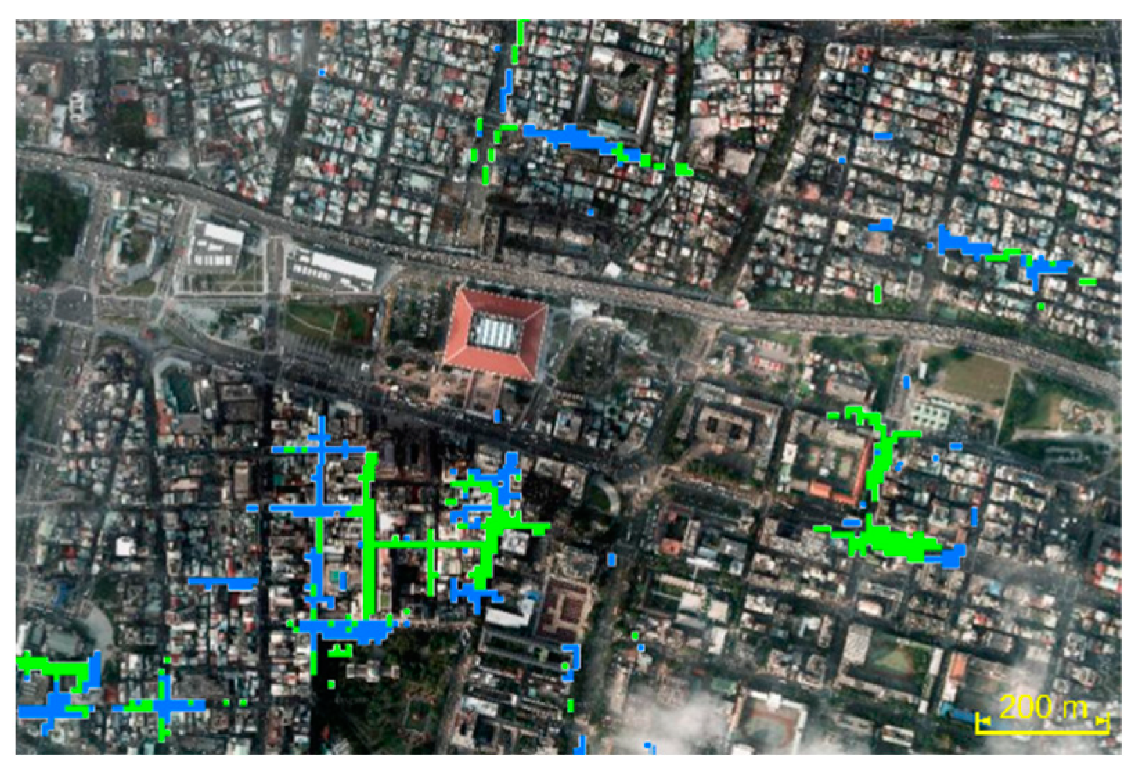
The flood inundation map of Taipei City in Fig. 2 illustrates that, under short-duration heavy rainfall, areas of high flood susceptibility are small and dispersed within the watershed. To mitigate flood damage in susceptible areas and provide timely warnings, an urban rainfall-runoff model capable of nowcasting is imperative. Such a model must be highly detailed to suit the urban landscape, as exemplified by models in Rodiguez et al. [4] and Amaguchi et al. [5], where the delineation between buildings and open spaces is clearly defined from urban geography databases. The rainfall-runoff calculation should scale down to the basic elements of an urban catchment, such as individual buildings or open spaces with distinct boundaries. However, the highly detailed delineation poses a challenge, generating a large number of runoff units. Utilizing a numerical model to calculate all these runoff units piece by piece would be time-consuming, rendering the model inappropriate for rainfall-runoff nowcasting. Therefore, to create a highly detailed urban rainfall-runoff model suitable for nowcasting, the calculation of each runoff unit must be more efficient to reduce the overall calculation time.

Addressing the challenges in flood nowcasting, a novel lumped model was purposed in [6,7] for flood nowcasting in Taiwan. Given the lack of complete observation records for river basins in their research and the highly variable nature of rainfall in Taiwan, traditional lumped models like the tank model from Sugawara [8] and Storage Function model from Kimura [9] are deemed unsuitable. This is due to the high variability of model parameters in different events, and the unit hydrograph, which is inappropriate for the runoff calculation in a river basin experiencing high-intensity rainfall events. The basin discharge under such conditions cannot be linearly transformed into a unit hydrograph, indicating a nonlinear rainfall-runoff process during high rainfall intensity events.

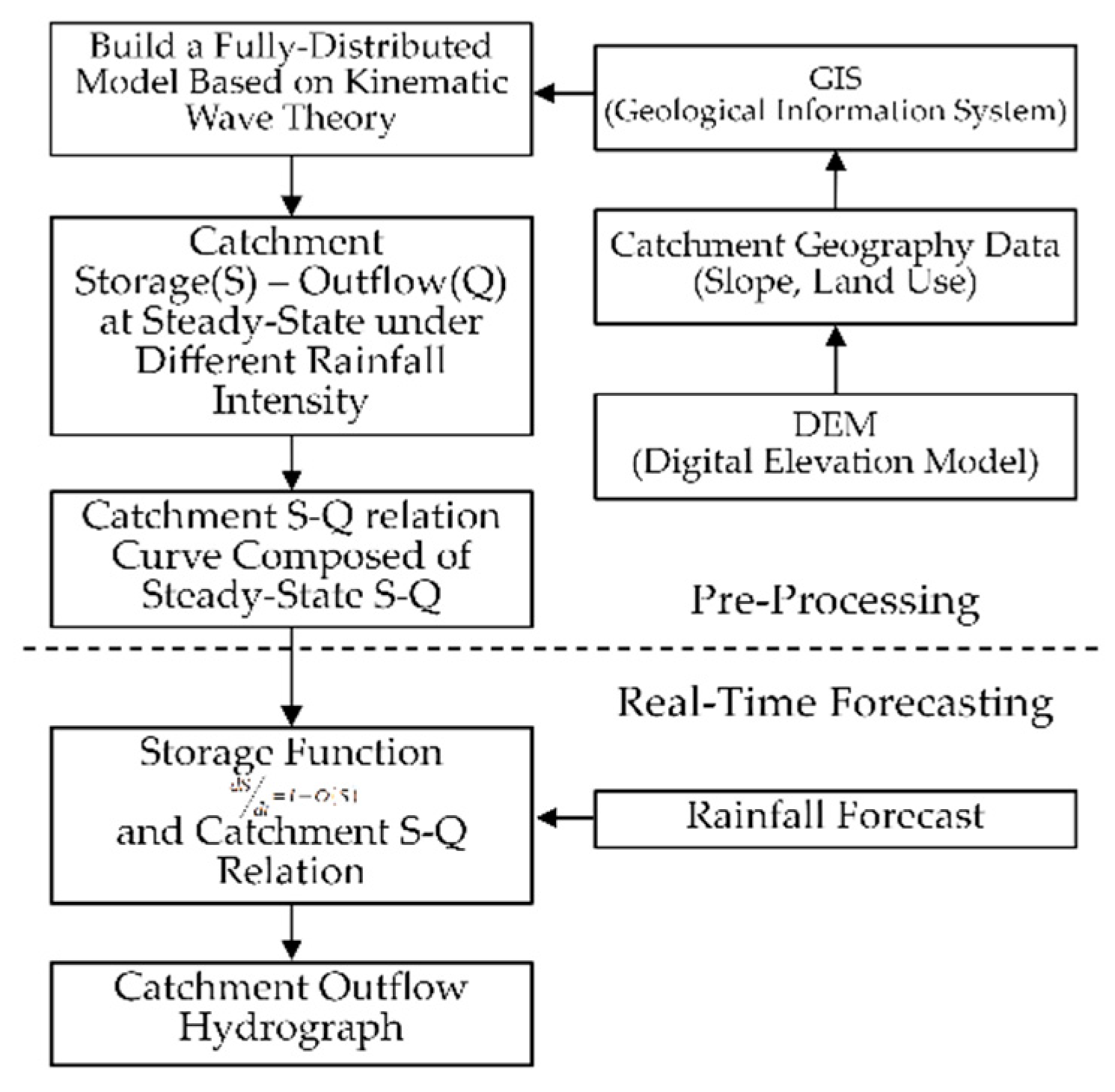
To overcome the complexities in flood nowcasting, the BKW model employs the process depicted in Fig. 4. In the pre-processing phase, a fully-distributed model based on the kinematic wave assumption is constructed to simulate the outflow process of the catchment. Assuming no infiltration and a fixed rainfall intensity, the model simulates the runoff of the catchment until it reaches a steady-state. The steady-state outflow and storage serve as a point in the storage-outflow relation of the catchment. Another event with a different fixed rainfall intensity is simulated to steady-state, generating another point on the catchment storage-outflow relation curve. By repeating this process with multiple events of varying fixed rainfall intensity, a storage-outflow relation curve is obtained. In the real-time forecasting phase, the catchment storage-outflow relation is utilized in a storage function. With forecasted rainfall as input, BKW efficiently simulates catchment runoff compared to a fully-distributed model. Unlike the Storage Function Model, the storage-outflow relation of BKW consists of discrete points from each event of fixed rainfall intensity. To obtain the catchment outflow, BKW interpolates on the storage-outflow curve using the current catchment storage, deviating from the traditional model, which describes the catchment storage-outflow relation through an equation derived from regression analysis of storage-discharge variation processes in previous catchment events.

Figure 3. Workflow chart for the Block Kinematic Wave model.

In scenarios where a sub-catchment possesses a distinct drainage gradient, and the course of runoff aligns with rather than opposes this slope, the kinematic wave model emerges as a viable approach for precise computation of rainfall-runoff dynamics within urban sub-catchments. The analytical solution of kinematic wave overland flow, as presented in Wooding [10] and Eagleson [11], assumes constant roughness and drainage slope. The solution describes the runoff generation of fixed rainfall intensity on an impervious, rectangular plane and the recession of the plane from steady-state. When applying a lumped model to simulate the rainfall-runoff of an urban sub-catchment, the outflow hydrograph should closely align with the analytical solution for the same event.

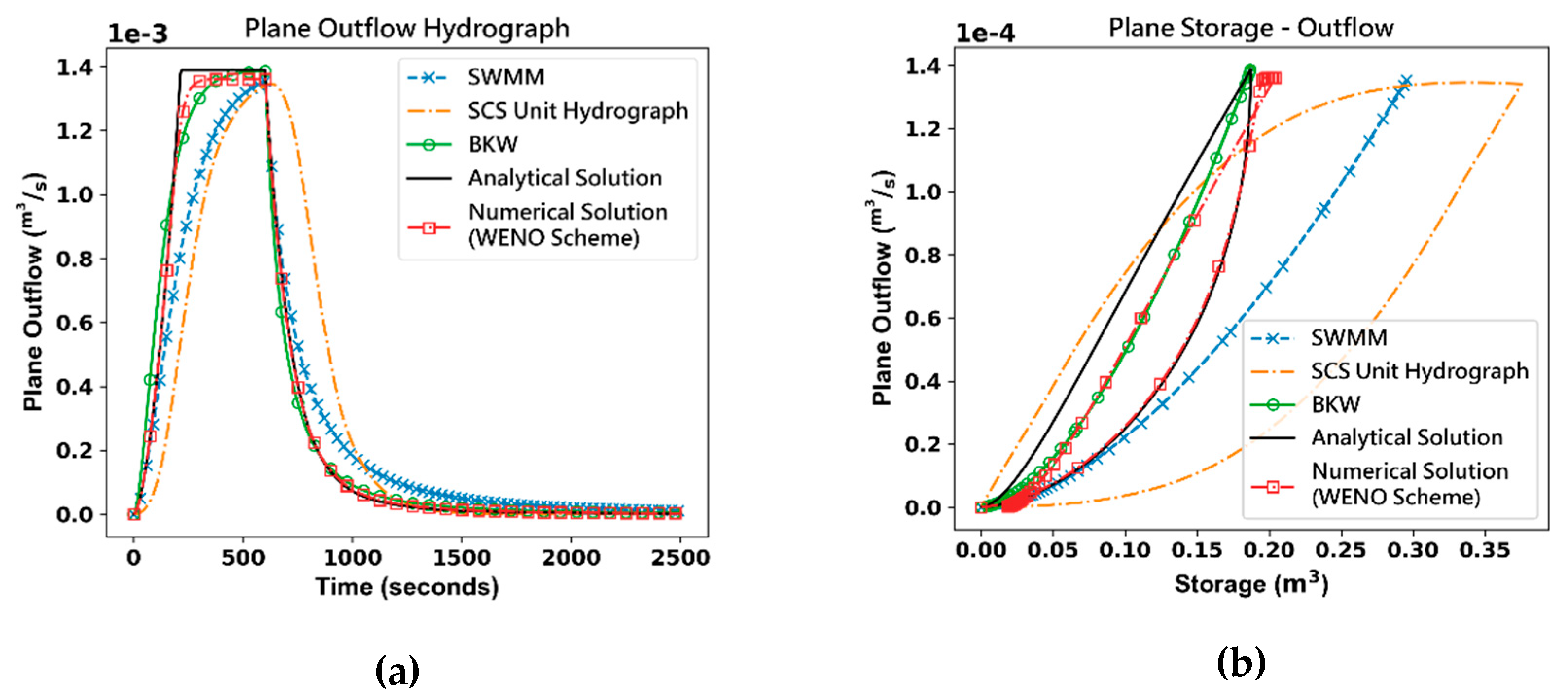
Assuming an impervious urban sub-catchment as Figure 4, where the rectangular plane is 20m in length and 10m in width, the slope of catchment is 0.005 and the manning roughness represented by 0.01. The outflow from this rectangular plane under constant rainfall can be derived through analytical solutions. This approach facilitates the testing and comparison of various runoff simulation methods for an urban sub-catchment against the results obtained through the analytical solution. Figure 5 illustrates the application of multiple rainfall-runoff models, including the SCS Unit Hydrograph, SWMM from Huber and Dickinson [12], and BKW, to evaluate the compatibility of these models in the context of an urban sub-catchment. Figure 5(a) presents the outflow of each model, comparing them with the WENO scheme from Yu and Duan [12]. Notably, all lumped methods in Figure 5(a) take more time to reach steady-state outflow and fail to generate an outflow hydrograph that exactly matches the analytical solution. Achieving accuracy in simulating high-intensity, short-duration rainfall on an urban sub-catchment requires the lumped rainfall-runoff method to provide results much closer to the analytical solution. A comparison of the storage-outflow relation of BKW to the analytical solution in Figure 5(b) reveals that the storage-outflow of the analytical solution exhibits obvious hysteresis behavior also the numerical solution, whereas BKW demonstrates a nonlinear curve.

The observation of hysteresis in the storage-outflow of overland flow has been documented by Holtan and Overton [13], Langford and Turner [14]. In Chung [15], purposed a hypothesis suggesting that storage-outflow hysteresis arises from the lag time in runoff transportation from upstream to downstream. To test this hypothesis, a rectangular catchment was divided into multiple parts from upstream to downstream. Each sub-catchment was calculated by BKW, and the outflow was transported downstream to the next sub-catchment, akin to the concept of a linear reservoir in series. The hypothesis proposed that more divided sub-catchments would take more time in the transportation of runoff, and the storage-outflow hysteresis should be more apparent in the catchment storage-outflow. However, the test results indicated that more divided sub-catchments did not generate hysteric storage-outflow in the simulation. Instead, they approached a single nonlinear storage-outflow curve, suggesting the failure of the hypothesis. The hysteresis in the storage-outflow of overland flow does not hinge on the lag time in the transport of runoff from upstream to downstream. Exploring why BKW in series does not exhibit storage-outflow hysteresis in the simulation may be attributed to the calculation mechanism of BKW. BKW’s calculation relies on integrating the storage function and interpolating the storage-outflow curve using the current catchment storage. This process entails solving an ordinary differential equation (ODE) of catchment storage and time. In contrast, the analytical solution or numerical solution to solve water depth and outflow involves position, water depth on the plane, and time differences, amounting to solving a partial differential equation (PDE) in the process.

A system exhibiting hysteresis, as mentioned in Gharari and Razavi [16], is characterized as either path-dependent or possessing memory. The system’s output is influenced not only by the current input but also by past inputs. Considering overland flow on an inclined plane as a hysteretic system, where the outflow from the plane serves as the system’s output and rainfall acts as the input, BKW’s outflow, solely correlated with the current rainfall input, categorizes BKW as a non-hysteretic system, lacking memory. In an attempt to develop a path-dependent Storage Function model, Wu [17] endeavored to use two sets of parameters to address the rising phase (increasing rainfall intensity) and the recession phase (decreasing rainfall intensity) in a rainfall event. This process involves identifying the rising and recession phases of an event, which can be challenging in highly variable rainfall events. To enhance the accuracy of the BKW model further, the model must be capable of reacting to past rainfall inputs, transforming it into a path-dependent model. Since the storage-outflow relation is the sole factor controlling the output of BKW, understanding how storage-outflow hysteresis forms in overland flow and how past rainfall affects the storage-outflow path on a plane is crucial to harnessing overland flow hysteresis for BKW improvement.

2. Methods

2.1. Overland flow from steady-state to steady-state

Assuming raindrops fall onto the rectangular plane similar to Figure 4, where the length of the plane is denoted as L, and horizontal positions on the plane are represented by x, with the plane having an inclined slope of S₀. The overland flow on the plane is calculated using the kinematic wave model in Eq. (1). In Eq. (1), the upper equation signifies the mass balance, and the lower equation represents the moment equation, where y represents the depth of the overland flow. The Manning equation can be applied in turbulent flow, where α is the runoff parameter of the plane. In Eq. (2), n represents the Manning roughness of the plane, and it is assumed that the roughness is uniform throughout the plane. In the characteristic solution of the kinematic wave, a characteristic moves forward at the speed c in Eq. (3).

\{\begin{matrix} \frac{\partial y}{\partial t} + \frac{\partial q}{\partial x} = i \\ q = α y^{m} \end{matrix}

(1)

α = \frac{1}{n} S_{0}^{\frac{1}{2}}

(2)

\frac{d x}{d t} = c = m α y^{m - 1}

(3)

While the plane is in a steady state under rainfall intensity i₁, with t > t₀, the rainfall intensity becomes i₂. As a characteristic starts from x₀ when t = t₀, the depth changes according to Eq. (4).

y = {(\frac{i_{1} x_{0}}{α})}^{\frac{1}{m}} + \int_{t_{0}}^{t} i_{2} d τ

(4)

And Eq. (5) is the characteristic.

x - x_{0} = m α \int_{t_{0}}^{t} {({(\frac{i_{1} x_{0}}{α})}^{\frac{1}{m}} + \int_{t_{0}}^{θ} i_{2} d τ)}^{m - 1} d θ

(5)

Integrate Eq. (5), we get Eq. (6)

x - x_{0} = \frac{α}{i_{2}} {({(\frac{i_{1} x_{0}}{α})}^{\frac{1}{m}} + i_{2} (t - t_{0}))}^{m} - \frac{i_{1}}{i_{2}} x_{0}

(6)

To reach steady-state under i₂, the characteristic originated from x=0 at t₀ must reach the length L, denoted as t_c in Eq. (7).

t_{c} = \frac{1}{i_{2}} {(\frac{i_{2} L}{α})}^{\frac{1}{m}}

(7)

Using the dimensionless variables in Eq. (8) to replace the variables in the equations above.

\begin{matrix} X = \frac{x}{L} Y = y \cdot {(\frac{i_{2} L}{α})}^{- \frac{1}{m}} T = t \cdot {(\frac{1}{i_{2}} {(\frac{i_{2} L}{α})}^{\frac{1}{m}})}^{- 1} \\ Q = \frac{q}{i_{2} L} γ = \frac{i_{1}}{i_{2}} \end{matrix}

(8)

Replace the variables in Eq. (6) to dimensionless variables.

X - X_{0} = {({(γ X_{0})}^{\frac{1}{m}} + (T - T_{0}))}^{m} - γ X_{0}

(9)

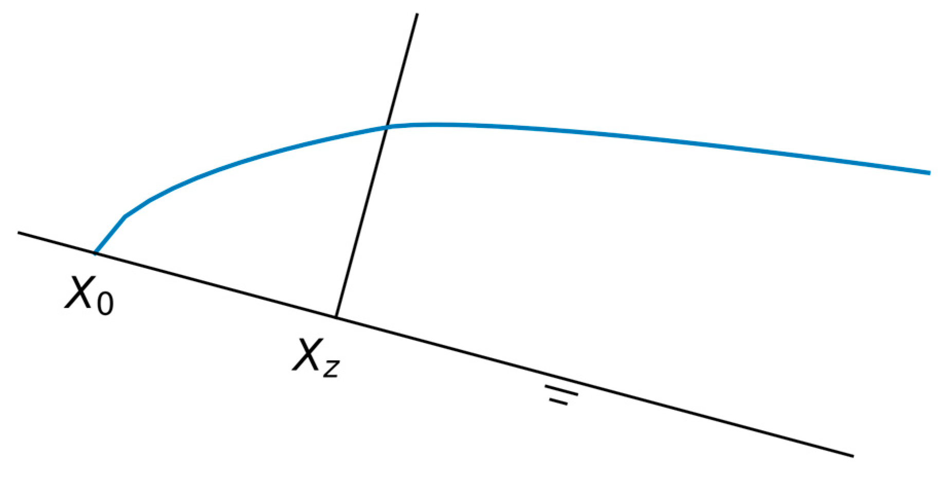
Started from X=0 at T=T₀, the characteristic moves forward to X_z by T. The region where X ≤ X_z on the plane, is under steady-state of rainfall intensity i₂, and the region X > X_z remains unsteady as the characteristics influenced by both the rainfall intensity i₁ and i₂, as shown in Figure 6.

X_{z} = {(T - T_{0})}^{m}

(10)

For any characteristics positioned at X > X_z by the time T, Eq. (6) can be used to track the X₀ where the characteristics originated. For the region where X ≤ X_z at time T, the overland flow depth is proportional to the position X on the plane, as Equation (11) below. For the depth on the position X where X > X_z, as X₀ is found using Equation (6), the depth is Eq. (12)

Y = X^{\frac{1}{m}}

(11)

Y = {(γ X_{0})}^{\frac{1}{m}} + (T - T_{0})

(12)

For X > X_z, employing the depth of overland flow in Eq. (12), the flowrate at X is

Q = {({(γ X_{0})}^{\frac{1}{m}} + (T - T_{0}))}^{m}

(13)

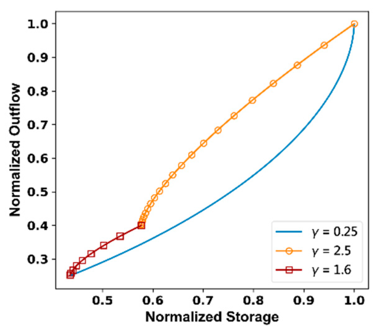
Using different γ, we have the storage-outflow relation curve illustrated in Figure 7 below.

2.2. Storage-Outflow Relation of Overland Flow in Shift Between Two Steady-State

In section 2.1, the derivation shows that the normalized outflow hydrograph of overland flow, as well as the storage-discharge (S-Q) relation, is determined by the ratio of rainfall intensity γ. This implies that the S-Q relationship on a plane during a rainfall event is dynamic, undergoing changes in response to variations in rainfall intensity. Ensuring the accuracy of catchment outflow estimations by the BKW model requires a close alignment of the model’s S-Q relation with that of the catchment. Given that changes in rainfall intensity also affect the catchment’s S-Q relation, the BKW model must dynamically adjust its S-Q relation to accurately estimate catchment outflow under varying rainfall intensities.

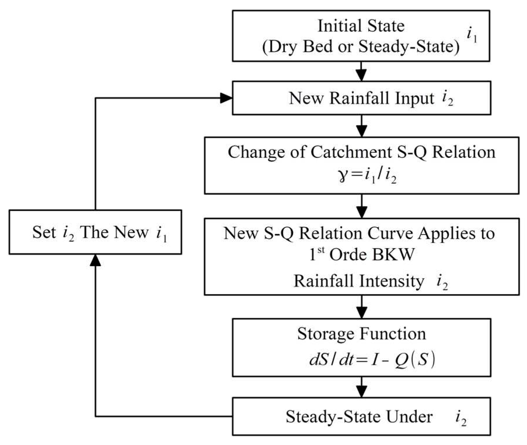
To discern how the BKW model modifies the S-Q relation in response to changes in rainfall intensity, the new model is denoted as the 1st order BKW model, distinguishing it from the 0th order BKW model where the S-Q relation is fixed. The change in the S-Q relation occurs when rainfall intensity shifts. Given a catchment simulated by the 1st order BKW, the S-Q relation of the catchment should change accordingly. In the 1st order BKW, the procedure in Figure 8 is used to simulate catchment runoff. Each time rainfall intensity changes, a new S-Q relation is generated by the ratio of the prior and the current rainfall intensity γ. The new S-Q relation is applied to the 1^st order BKW. As the catchment reaches steady-state, the outflow and storage remain constant until the next change in rainfall intensity occurs. By using the procedure, the S-Q relation in the 1st order BKW follows the S-Q relation in the catchment. The past and current rainfall intensity mutually influence the output of the catchment.

2.3. Normalize the S-Q curves

For a model to be used in real-time forecasting, calculation efficiency is important to provide timely simulation results. As the catchment S-Q relation changes along with the change in rainfall intensity, each time the rainfall intensity changes, a new S-Q relation curve is required. Using an analytical solution to iteratively derive the S-Q relation in each change of rainfall intensity would be time-consuming in real-time applications. Therefore, we need a new method to obtain the S-Q relation curve for the given gamma with less computational cost. A viable strategy is to parameterize the S-Q curves of various gamma values; the parameters can be interpolated and used to generate an S-Q curve for a given γ.

To model the S-Q relation curves, a cubic Bezier curve emerges as a judicious choice. The Bezier curve has clear start and end points, aligning well with the characteristics of the S-Q relation curves. Additionally, it is easy to adjust the curvature of a cubic Bezier curve to fit the S-Q relation curves.

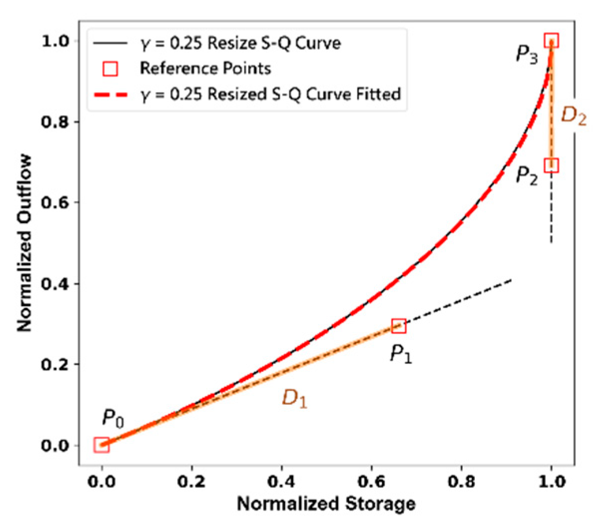
Eq. (14) is the governing equation of cubic Bezeir curve, consists of four control points P₀~P₃ and parameter z in range between (0, 1). P₀ and P₃ is equivalent to the start and end point of the S-Q curve. By adjusting the positions of P₁ and P₂, the Bezier curve can exhibit an appropriate curvature, effectively fitting the S-Q curve.

B (z) = {(1 - z)}^{3} P_{0} + 3 {(1 - z)}^{2} z \cdot P_{1} + 3 (1 - z) z^{2} \cdot P_{2} + z^{3} P_{3}

(14)

Resize the S-Q curve with Eq. (15), where the S-Q curve is stretched or compressed to the range (0, 0) and (1, 1). In Eq. (15), denote

S_{j}

and

Q_{j}

the storage and outflow on the S-Q curve,

S_{j}^{'}

and

Q_{j}^{'}

the resized storage and outflow, where

S_{i_{1}}

denote the steady-state storage under

i_{1}

, and

Q_{i_{1}}

denote the steady-state outflow under

i_{1}

\begin{matrix} S_{j}^{'} = \frac{S_{j} - \min (S_{i_{1}}, S_{i_{2}})}{\max (S_{i_{1}}, S_{i_{2}}) - \min (S_{i_{1}}, S_{i_{2}})} \\ Q_{j}^{'} = \frac{Q_{j} - \min (Q_{i_{1}}, Q_{i_{2}})}{\max (Q_{i_{1}}, Q_{i_{2}}) - \min (Q_{i_{1}}, Q_{i_{2}})} \end{matrix}

(15)

Let D₁ represent the distance between P₀ and P₁, and D₂ the distance between P₂ and P₃. The slope of the vector

\vec{P_{0} P_{1}}

is equal to the tangent of the resized S-Q curve at the starting point, and the slope of the vector

\vec{P_{3} P_{2}}

is equal to the tangent at the endpoint of the curve. Through the use of optimization methods, the optimal values for D₁ and D₂ can be determined, ensuring that the cubic Bezier curve maximally resembles the resized S-Q curve. In Figure 10 below, cubic Bezeir curve is used to fit a γ = 0.25 resized Bezeir curve, by adjusting D₁ and D₂, the cubic Bezeir presents adequate curvature to fit the resized S-Q curve.

Figure 9. γ = 0.25 Resized S-Q curve fitted by cubic Bezeir Curve.

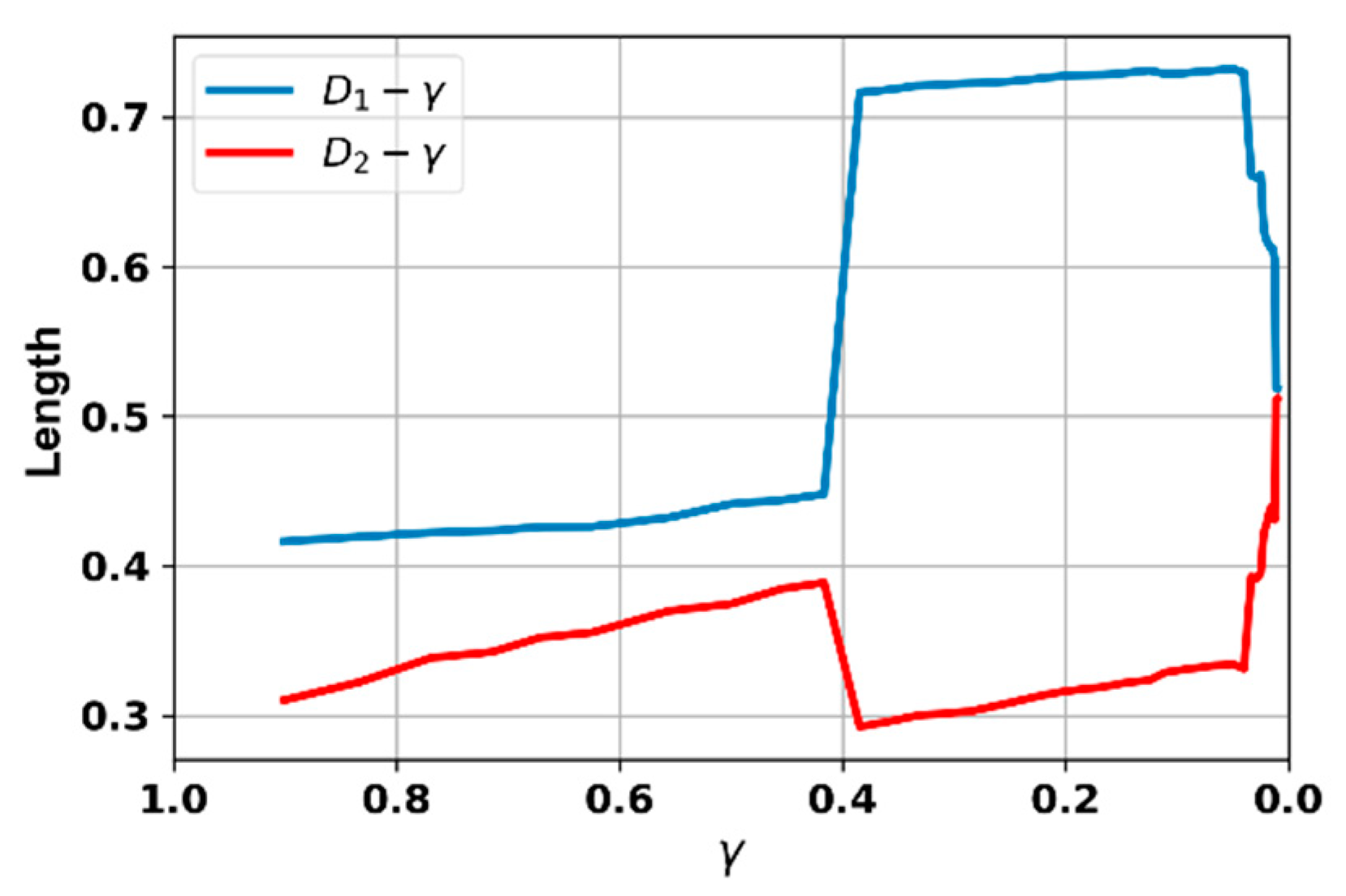
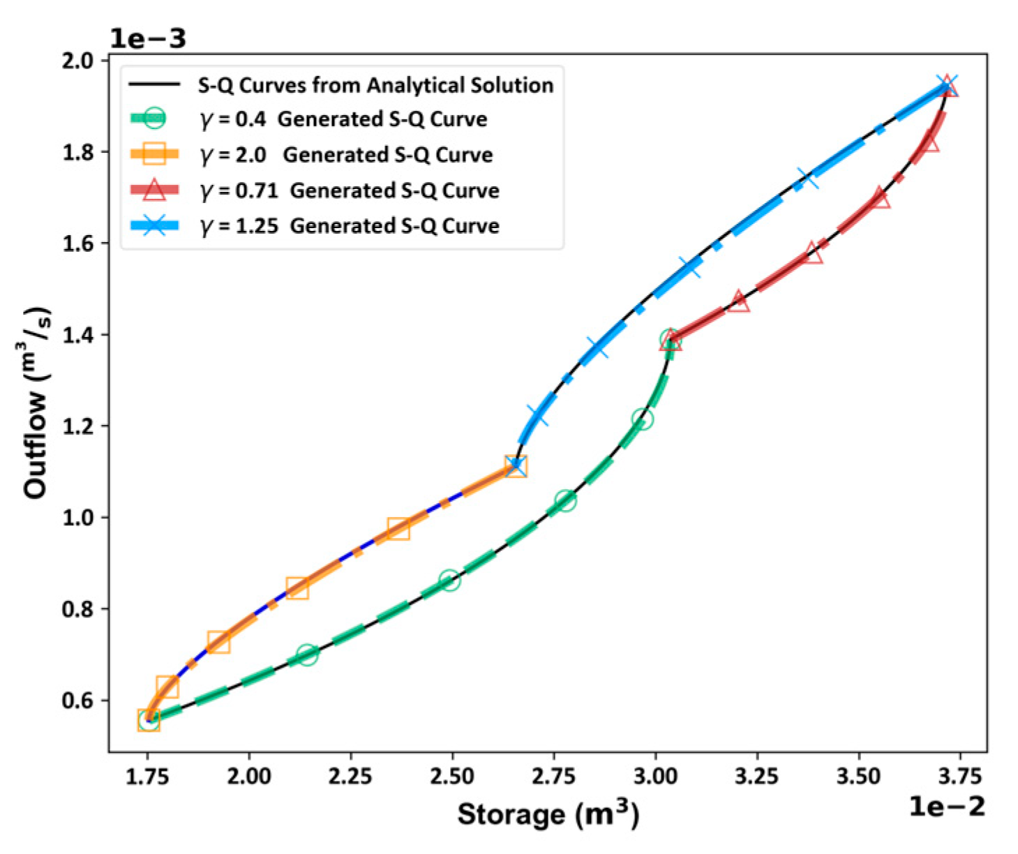
With multiple resized S-Q curves fitted by cubic Bezier curves, the D₁-γ and D₂-γ relation can be built, as illustrated in Figure. 10. To generate an S-Q curve for a given γ, instead of using the analytical solution, a cubic Bezier curve can be employed, as it can fit the resized S-Q curve. The four reference points of the cubic Bezier curve have to be determined prior to curve generation. Since the resized S-Q curve has fixed starting and ending points, only P₁ and P₂ need to be determined. With the given γ, D₁ and D₂ values can be obtained through the interpolation of the D₁-γ and D₂-γ relation. The tangent at the starting point and ending point of a resized S-Q curve can be obtained through the calculation of Eq. (13) and (15). Extend D₁ from P₀ by the tangent at the resized S-Q curve’s starting point, position P₁, and extend D₂ from P₃ by the tangent at the endpoint, position P₂. Using the four reference points and Eq. (14) to generate the Bezier curve, we obtain an approximation curve closely resembling the resized S-Q curve for the given γ, as depicted in Figure 11.

3. Results

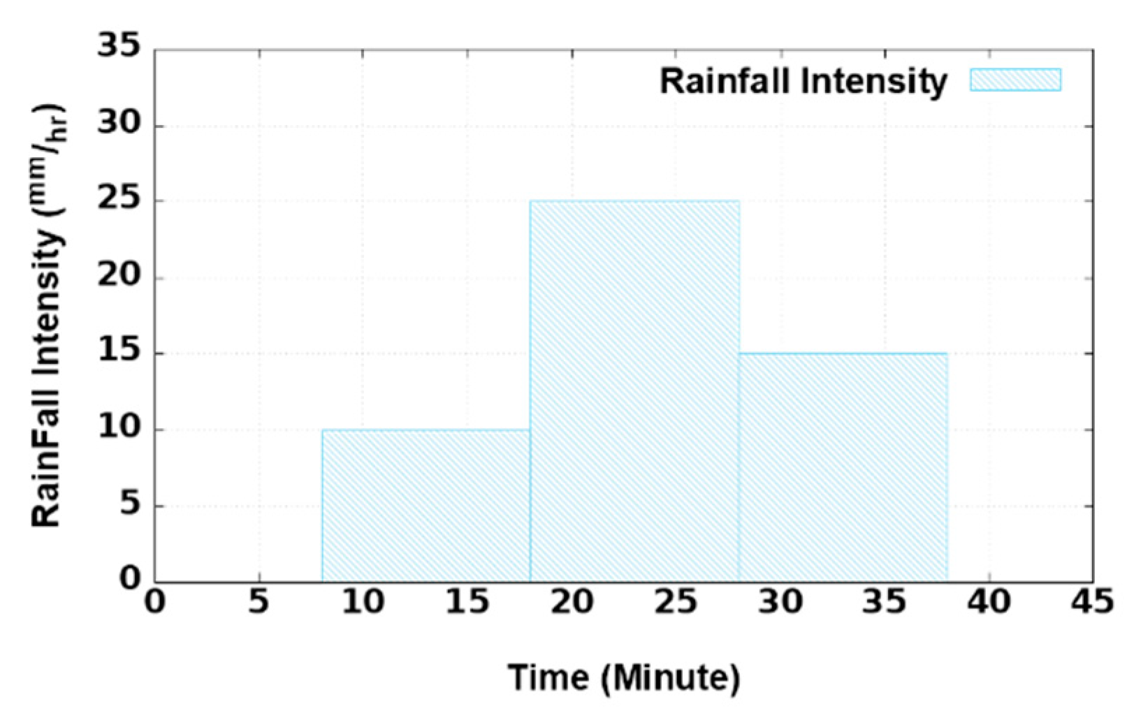
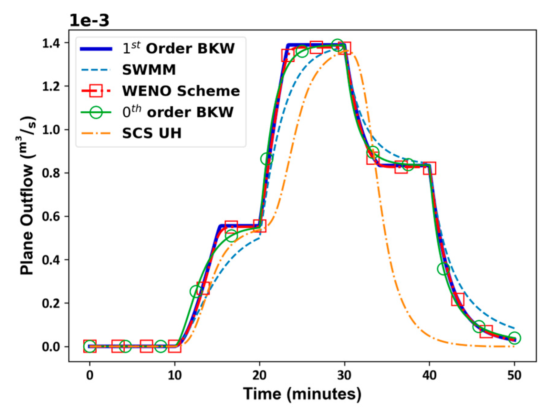
The 1^st order BKW uses a dynamic S-Q relation in simulation, distinguishing it from other Storage Function-type lumped models that utilize a fixed S-Q relation in rainfall-runoff computations. In the first-order BKW model, the S-Q relation dynamically adjusts with variations in rainfall intensity, generating a new S-Q relation applied through the procedural steps illustrated in Figure 8. Using the rectangular plane in Figure 4 and the rainfall hydrograph in Figure 12, we conducted simulations utilizing multiple lumped rainfall-runoff models, including the 1^st order BKW and 0^th order BKW, to compare the model efficiency of each model. A comparative analysis ensued, contrasting the simulated outflow hydrograph with the hydrograph produced by the WENO scheme. On an Intel i7-9750 system with 16 GB RAM, we further examined the calculation times of each model, he resulting outflow hydrographs of the lumped models are visually presented in Figure 13, accompanied by the numerical model’s hydrograph. The efficiency of each lumped model is quantified using the Nash-Sutcliffe Efficiency Coefficient (NSE) in Eq. (16), as detailed in Table 1, along with the respective calculation times.

N S E = \frac{\sum_{j = 1}^{N} (Q_{o}^{j} - Q_{m}^{j})}{\sum_{j = 1}^{N} (Q_{o}^{j} - \bar{Q_{o}})}

(16)

As shown in Table 1, the first-order BKW boasts the highest model efficiency among the lumped models. Despite requiring additional calculation time to adapt to the dynamic S-Q relation in the procedural steps, the necessary computation time is significantly reduced, and the simulated hydrograph closely mirrors the numerical model. As depicted in Figure 13, the numerical model attains a steady state, maintaining constancy as the rainfall intensity persists. In each 10-minute interval, the 1^st order BKW also achieves a steady-state outflow, echoing the behavior of the numerical model. Conversely, the 0^th order BKW takes more time to reach steady-state but other models fail to reach steady-state outflow.

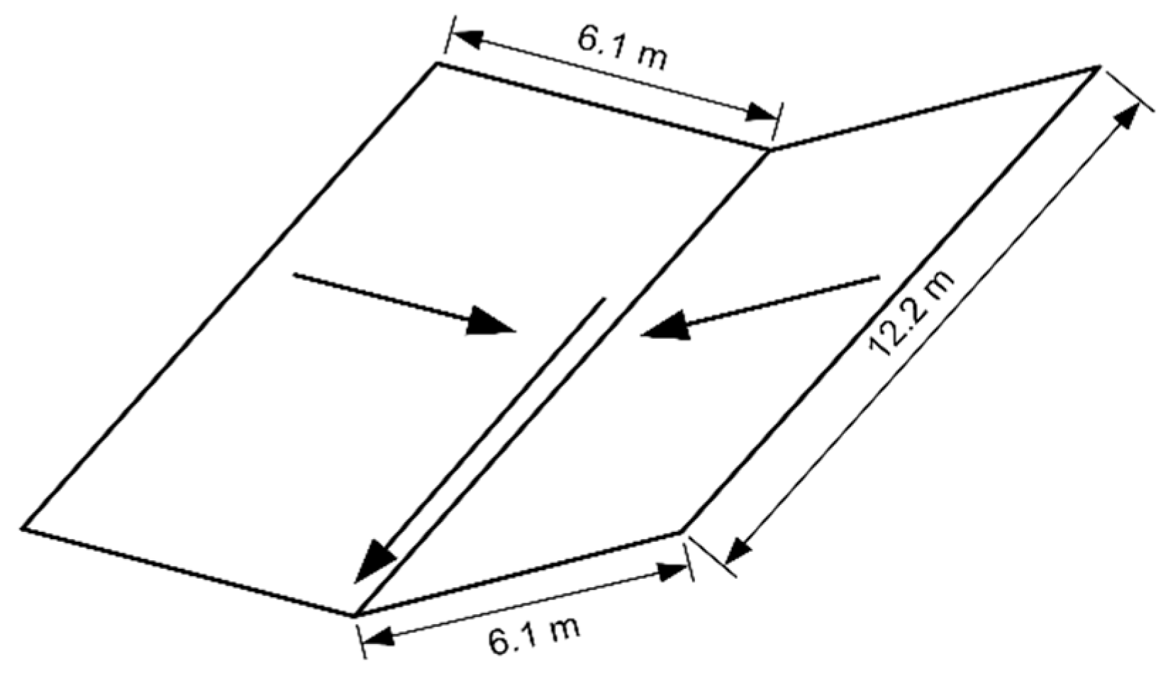
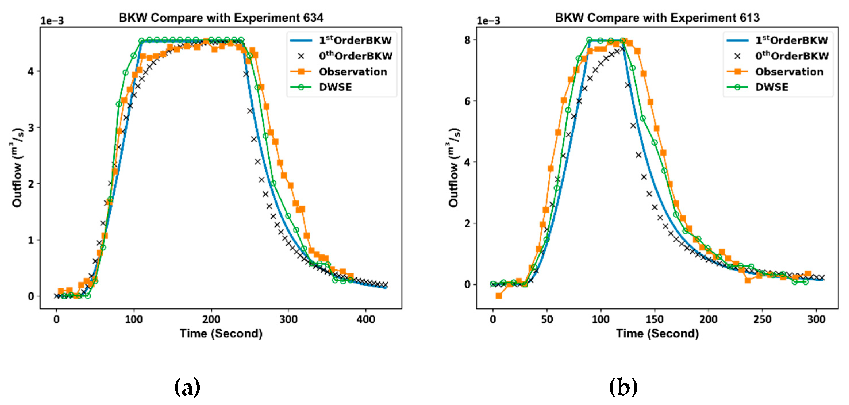
In evaluating the BKW’s performance within a watershed encompassing both catchment and channel elements, the model is applied to the experimental watershed illustrated in Figure 14 to compare with the experiment data in [18]. In the experiment 634 and the experiment 613, the slope of catchment and channel are both set to 0.01. In experiment 634, an event featuring a rainfall intensity of 109.6 mm/hr and a duration of 240 seconds applied to the experimental watershed. Applying identical conditions, the BKW model simulated the runoff of the experimental watershed, and the resulting outflow hydrograph is presented in Figure 15(a), along with the experiment data and DWSE data of the experiment 634. In experiment 613, a fixed rainfall intensity of 192 mm/hr over a duration of 120 seconds was imposed on the experimental watershed. Utilizing the BKW model to simulate this rainfall event, the resultant outflow hydrograph is showcased in Figure 15(b) alongside the experiment data. Model efficiency of the BKW model, in comparison to the experimental data, is assessed using NSE and reported in Table 2.

Table 2 illustrates a marginally superior performance of the 1^st order BKW over the 0^th order BKW. In Figure 15(a), the 1^st order BKW reaches a steady state by 110 seconds, closely mirroring the DWSE model, whereas the 0^th order BKW takes 200 seconds to achieve steady-state outflow. Additionally, in Figure 15(b), the 1^st order BKW attains a steady state within 90 seconds, whereas the 0^th order BKW fails to reach a steady state within 120 seconds. Figure 15(a) and Figure 15(b) reveal that the 1st order BKW’s outflow hydrograph closely aligns with the DWSE model, although displaying some variations in the phase from dry bed to steady-state. Given the composite nature of the watershed, encompassing both catchment and channel elements, the S-Q relation may differ from the S-Q relation derived solely from overland flow. Further investigation is necessary to explore these distinctions in the S-Q relation within the watershed and catchment.

4. Summary and Conclusions

In this research, an analytical solution was derived to elucidate the relationship between storage (S) and outflow (Q) in overland flow on an impervious plane. The study reveals that this S-Q dynamic is predominantly influenced by variations in rainfall intensity. The alteration in the intensity of rainfall governs the trajectory of the S-Q relationship, with the ratio of past to current rainfall intensity playing a pivotal role. This ratio, in turn, delineates a distinctive S-Q pathway.

In response to the dynamic changes in the S-Q relationship resulting from fluctuations in rainfall intensity, the BKW model employs a variable S-Q relation to achieve precise outflow estimation. Through the application of this variable S-Q relation in the BKW model, due consideration is given to the impact of past rainfall inputs on the current model output. This incorporation of past rainfall data leaves a memory in the BKW model, rendering it path-dependent. The resultant model, distinguished by its inherent path-dependent characteristics that set it apart from the original BKW model, denoted as the 1^st order BKW model.

The 1^st order BKW model establishes itself as a viable solution for real-time forecasting of rainfall-runoff in urban catchments, particularly those featuring a high proportion of impervious pavement and relatively brief time of concentration. In such environments, the 1st order BKW model demonstrates high accuracy in simulating runoff outcomes, accomplishing this with significantly reduced computational time compared to numerical models.

However, it is essential to note that the applicability of the 1st order BKW model is constrained to small sub-catchments or small watersheds where steady-state conditions can be achieved during each fluctuation in rainfall intensity. This limitation restricts the utilization of the 1^st order BKW model to relatively small, impervious sub-catchments. Further research efforts are imperative to expand and refine the application of the BKW model for broader usage, enhance its adaptability to diverse hydrological scenarios.

References

Chen, T.-C.; Tsay, J.-D.; Takle, E.S. A Forecast Advisory for Afternoon Thunderstorm Occurrence in the Taipei Basin during Summer Developed from Diagnostic Analysis. Weather and Forecasting 2016, 31, 531–552. [Google Scholar] [CrossRef]
Miao, J.-E.; Yang, M.-J. A Modeling Study of the Severe Afternoon Thunderstorm Event at Taipei on 14 June 2015: The Roles of Sea Breeze, Microphysics, and Terrain. Journal of the Meteorological Society of Japan. Ser. II 2020, 98, 129–152. [Google Scholar] [CrossRef]
Lin, C.-Y.; Chen, W.-C.; Chang, P.-L.; Sheng, Y.-F. Impact of the Urban Heat Island Effect on Precipitation over a Complex Geographic Environment in Northern Taiwan. J. Appl. Meteor. Climatol. 2010, 50, 339–353. [Google Scholar] [CrossRef]
Rodriguez, F.; Andrieu, H.; Creutin, J.-D. Surface Runoff in Urban Catchments: Morphological Identification of Unit Hydrographs from Urban Databanks. Journal of Hydrology 2003, 283, 146–168. [Google Scholar] [CrossRef]
Amaguchi, H.; Kawamura, A.; Olsson, J.; Takasaki, T. Development and Testing of a Distributed Urban Storm Runoff Event Model with a Vector-Based Catchment Delineation. Journal of Hydrology 2012, 420–421, 205–215. [Google Scholar] [CrossRef]
Hu, S.-H. Developing Block Kinematic Wave Model for Direct Runoff Hydrograph Estimate. master’s thesis, National Taiwan University: Taipei, 2011.
Yu, H.-L. The study of hydrological improvement of Block Kinematic Wave Model. Master Thesis, National Taiwan University: Taipei, 2013.
Sugawara, M. Tank Model. Journal of Geography (Chigaku Zasshi) 1985, 94, 209–221. [Google Scholar] [CrossRef]
Kimura, T. The Flood Runoff Analysis Method by the Storage Function Model. The Public Works Research Institute, Ministry of Construction, Japan 1961.
Wooding, R.A. A Hydraulic Model for the Catchment-Stream Problem: I. Kinematic-Wave Theory. Journal of Hydrology 1965, 3, 254–267. [Google Scholar] [CrossRef]
Eagleson, P.S. Surface Runoff And Streamflow. In Dynamic hydrology; McGraw-Hill, 1970; pp. 325–367 ISBN 978-3-936586-09-1.
Yu, C.; Duan, J.G. High Resolution Numerical Schemes for Solving Kinematic Wave Equation. Journal of Hydrology 2014, 519, 823–832. [Google Scholar] [CrossRef]
Holtan, H.N.; Overton, D.E. Storage-Flow Hysteresis in Hydrograph Synthesis. Journal of Hydrology 1965, 2, 309–323. [Google Scholar] [CrossRef]
Langford, K.J.; Turner, A.K. An Experimental Study of the Application of Kinematic-Wave Theory to Overland Flow. Journal of Hydrology 1973, 18, 125–145. [Google Scholar] [CrossRef]
Chung, W.-C. An Error Analysis Study on Block Kinematic Wave Direct Runoff Model. Master Thesis, National Taiwan University: Taipei, 2016.
Gharari, S.; Razavi, S. A Review and Synthesis of Hysteresis in Hydrology and Hydrological Modeling: Memory, Path-Dependency, or Missing Physics? Journal of Hydrology 2018, 566, 500–519. [Google Scholar] [CrossRef]
Wu, S.-J.; Ho, L.-F.; Yang, J.-C. Application of Modified Nonlinear Storage Function on Runoff Estimation. Journal of Hydro-environment Research 2011, 5, 37–47. [Google Scholar] [CrossRef]
Xiong, Y.; Melching, C. Comparison of Kinematic-Wave and Nonlinear Reservoir Routing of Urban Watershed Runoff. J. Hydrol. Eng. 2005, 10, 39–49. [Google Scholar] [CrossRef]

Figure 2. Part of the flood hazard map of Taipei City, Taiwan under short duration, high intensity rainfall. The colored area represents the inundation zone.

Figure 4. A test rectangular plane of fixed length.

Figure 5. Comparison of outflow hydrograph simulations for a rectangular plane under 25 ^mm/_hr, 10-minute duration rainfall, using various simulation methods. (a) The outflow hydrograph (b) The storage-outflow relation in the simulation.

Figure 6. The distribution of overland flow depth on a plane during the transition from one steady state to another, X_z separates the region that has reached steady state under rainfall intensity i₂ from the region that has not yet reached steady state.

Figure 7. Normalized Storage-Outflow relation of different γ.

Figure 8. Calculation procedure of 1^st order BKW model.

Figure 10. The D₁—γ and D₂—γ relation of resized S-Q curves.

Figure 11. Comparison of S-Q curves generated by cubic Bezier curve and the S-Q curves derived from analytical solution.

Figure 12. A simple rainfall hydrograph with 4 times of rainfall intensity changes.

Figure 13. Different outflow hydrographs generated by various rainfall-runoff models using the rainfall input in Figure 8.

Figure 14. The experimental catchment.

Figure 15. The experiment data from Xiong [18] compared with simulated watershed outflow by BKW (a) Experiment 634 of rainfall intensity 109 ^mm/_hr with 240-second in duration. (b) Experiment 613 of rainfall intensity 192.6 ^mm/_hr with 120-second in duration.

Table 1. Comparison of calculation time used in simulation of different methods using rainfall hydrograph in Figure 8.

Methods	Calculation Time (second)	NSE
1^st order BKW	0.278	0.999
0^th order BKW	0.058	0.996
SCS Unit Hydrograph	0.036	0.674
SWMM	0.22	0.975
WENO Scheme (Numerical Method)	25.56	—

Table 2. Model efficiency of BKW in reproducing experiment in Xiong [18] through simulation of BKW.

Model	Experiment 634	Experiment 613
1^st order BKW	0.912	0.864
0^th order BKW	0.850	0.829

Disclaimer/Publisher’s Note: The statements, opinions and data contained in all publications are solely those of the individual author(s) and contributor(s) and not of MDPI and/or the editor(s). MDPI and/or the editor(s) disclaim responsibility for any injury to people or property resulting from any ideas, methods, instructions or products referred to in the content.

© 2024 by the authors. Licensee MDPI, Basel, Switzerland. This article is an open access article distributed under the terms and conditions of the Creative Commons Attribution (CC BY) license (http://creativecommons.org/licenses/by/4.0/).

Copyright: This open access article is published under a Creative Commons CC BY 4.0 license, which permit the free download, distribution, and reuse, provided that the author and preprint are cited in any reuse.

MDPI Initiatives

Important Links

Choose an area of interest and we will send you notifications of new preprints at your preferred frequency.

Disclaimer

Block Kinematic Wave, A Novel Rainfall-Runoff Model For Small Urban Catchments

Abstract

1. Introduction

2. Methods

2.1. Overland flow from steady-state to steady-state

2.2. Storage-Outflow Relation of Overland Flow in Shift Between Two Steady-State

2.3. Normalize the S-Q curves

3. Results

4. Summary and Conclusions

References

MDPI Initiatives

Important Links

Subscribe