1. Introduction
The crucial role of transportation in everyday life, coupled with the limited capacity of transportation routes and the imperative to prevent accidents, underscores the significance of transportation planning. However, effective transportation planning is contingent upon having accurate road traffic information[1, 2]. Transportation plays a crucial role in modern society[
3], and efficient traffic flow management is essential for ensuring the smooth operation of highways. Predicting traffic flow is a key component of effective traffic management, aiding in the prevention of congestion, reduction of travel time, and enhancement of overall transportation efficiency. Traditional methods of traffic prediction have relied on simulation and statistical approaches based on mathematical relationships. In recent years, artificial neural networks (ANNs) have emerged as powerful tools for predicting complex and dynamic systems The significance of Artificial Intelligence (AI) in the field of computer science, particularly within the era of big data, cannot be overstated. Over the past 50 years, AI has made remarkable strides, particularly in machine learning, data mining, computer vision, expert systems, natural language processing, robotics, and various applications[
4]. Initially introduced in 1958[
5] and later refined in 1986[
6], ANNs have gained prominence for their ability to analyze and learn patterns from available data, providing valuable insights for predicting future outcomes[
7]. Indeed, short-term traffic flow prediction serves as a pivotal component of Intelligent Transportation Systems (ITS). This crucial function contributes to various aspects of transportation management, including traffic planning, control, and management. Additionally, it plays a vital role in supporting roadway safety evaluation and estimating energy consumption[
8].By unraveling these complexities, researchers and policymakers gain valuable insights that can guide informed decision-making and contribute to the development of sustainable, health-conscious urban environments[
9]. The advent of artificial intelligence (AI) approaches has paralleled the rapid development of new traffic flow prediction models and frameworks within the ITS[
10].
This study focuses on the design and implementation of an ANN model for predicting traffic flow in highways, with a specific emphasis on short-term predictions. The short-term aspect is particularly relevant for real-time traffic management.By leveraging historical data from a traffic counter station, this research aims to train an ANN using a multilayer perceptron approach. The trained network will then be tested for its accuracy in predicting traffic and speed for the upcoming week. The comparison between the predicted and recorded data, and statistical methods will be employed to assess the model's performance. This approach aims to utilize available data, extracting pertinent patterns to predict and derive suitable data in comparison to the patterns acquired during training. The primary objective of this article is to explore and ascertain the prediction of traffic .
2. Literature Review
Traffic congestion is a significant issue that affects transportation systems in both developed and developing countries. It can lead to increased travel times, reduced fuel efficiency, and increased emissions. Traffic control systems are designed to minimize traffic congestion and maximize traffic flow. However, effective traffic control requires accurate traffic flow data. This is where artificial neural networks (ANNs) can play a valuable role[
11]. traffic flow prediction has relied on human expertise, which can be subjective and limited by the availability of real-time data. This approach often fails to capture historical trends, seasonal patterns, and other factors that can significantly impact traffic patterns.Artificial neural networks (ANNs) offer a promising alternative for traffic flow prediction in Istanbul. ANNs are powerful machine learning algorithms inspired by the structure and function of the human brain. They can learn from large amounts of data, identify complex patterns, and make predictions with a high degree of accuracy. In the study, ANNs were used to predict traffic volume in major junctions across Istanbul. The model was trained on historical traffic data, including time of day, day of the week, holidays, school timings, and other relevant factors. The results were highly encouraging, demonstrating that ANNs can effectively capture the complex dynamics of Istanbul's traffic flow[
12]. Real-time traffic flow prediction is a crucial component of intelligent transportation systems (ITS). However, accurately predicting short-term traffic flow remains a challenging task due to the complexity and stochastic nature of traffic patterns. To address this issue, a novel combined prediction method for short-term traffic flow is proposed. This method leverages the autoregressive integrated moving average (ARIMA) model and the long short-term memory (LSTM) neural network to capture both linear and nonlinear patterns in traffic data[
13]. Traffic congestion has been a major problem in Italy, particularly in Rome. To address this issue, a Levenberg-Marquardt (LM) artificial neural network heuristic model was developed to predict traffic flow for non-autonomous vehicles. Traffic data was collected using inductive loop detectors and video cameras. The data was then used to train, test, and validate the LM model. The model achieved training, test, and regression values (R2) of 0.99892, 0.99615, and 0.99714, respectively. These results suggest that the LM model is a promising tool for predicting traffic flow in Italy[
14].
Despite the development of deep neural networks for traffic flow modeling, predicting citywide traffic flow at a fine temporal scale remains challenging, attributed to spatiotemporal dependencies and spatial sparsity. A study proposes a high-accuracy deep learning-based spatiotemporal neural network model after analyzing traffic flow patterns. The approach involves transforming the road network into a compact 2D image, representing road segments as pixels and preserving topological relationships. The end-to-end deep learning structure incorporates a recurrent convolutional network for temporal dependencies and a densely connected convolutional network for spatial dependencies and spatial sparsity. The model aggregates hybrid network outputs with different weights, enhanced by external information like the day of the week[
15]. A study on short-term traffic flow forecasting in undivided two-lane highways in India. The authors propose a back propagation artificial neural network (ANN) model for this purpose and compare its performance with several other machine learning models, including random forest, support vector machine, k-nearest neighbor classifier, regression tree, and multiple regression. The results show that the ANN model outperforms the other models, achieving an R-squared value of 0.9962[
16]. LSTM is a type of Recurrent Neural Network (RNN) specially designed to handle the temporal dependencies in sequential data, making it well-suited for traffic flow prediction, which is a time-series problem. The authors compare the performance of LSTM models trained with different input settings, including flow, speed, and occupancy data from the same detector station, and upstream and downstream detector stations. The results show that LSTM models that include both downstream and upstream traffic information are most accurate. This suggests that considering the spatial context of traffic flow, in addition to the temporal dynamics, is important for improving prediction accuracy[
13].
3. Research Method
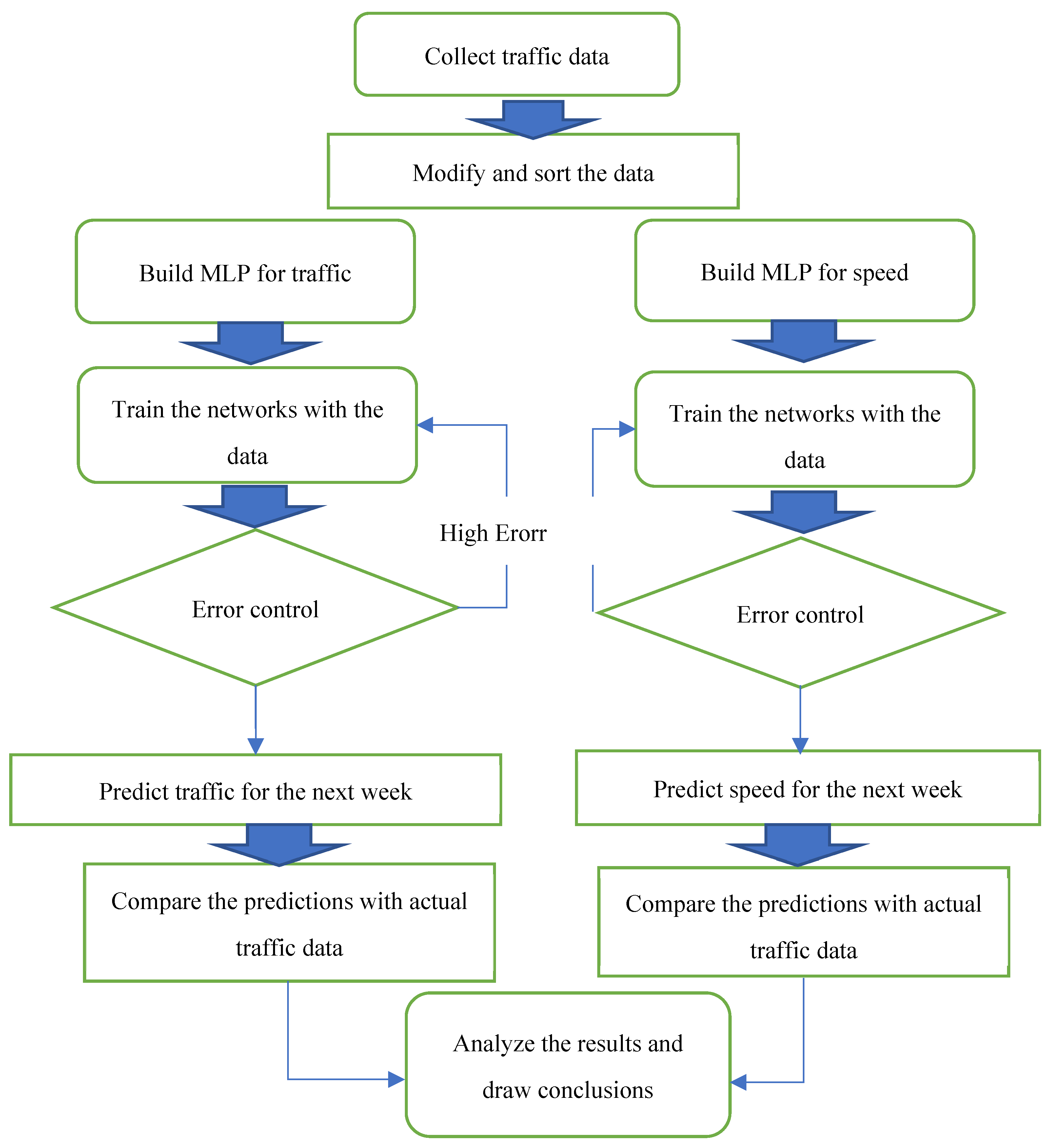
The research method used in this study involved collecting traffic data from the Tehran -Karaj highway, modifying and sorting the data, building neural network models for traffic and speed, training the networks with the data, predicting traffic for the next week using the models, and comparing the predictions with actual traffic data.
Figure 1 outlines the process flow of the proposed method. The first step involves data collection, gathering information from traffic counters. The acquired data undergoes modification and sorting to ensure consistency and completeness. This is crucial as traffic counters may experience downtime due to power outages or other technical disruptions, resulting in missing data. To address this issue and homogenize the data, an averaging approach is employed. For instance, if a traffic counter records 45 minutes of data but requires 60 minutes, the missing data is interpolated using a data ratio. This method ensures minimal data loss, with less than 1% error in the overall dataset.
Next, two neural network models are constructed: one for predicting traffic patterns and the other for forecasting traffic speeds. The models are trained using the processed data, generating an error output. This output serves as the basis for evaluating the model's performance. The model's structure and associated neurons are iteratively adjusted until the error rate reaches its minimum value. Following the development of the optimal model, its predictive capabilities are evaluated by simulating future traffic conditions for the upcoming week. MATLAB software is utilized for this simulation. The output obtained from the model is then compared with real-traffic data (traffic meter readings) to calculate the error variance.Finally, the conclusion is drawn, and the accuracy of the prediction is assessed. This evaluation encompasses both the model's ability to accurately predict traffic patterns and its effectiveness in forecasting traffic speeds.
In the neural network prediction process, the selection of the model, the number of neurons, and the activation function are crucial factors. Defining the model involves specifying input parameters, and in this context, two parameters are considered:
P1: The code representing the days in a month, ranging from 1 to 31.
P2: Traffic hours in a day, corresponding to the 24 hours in a day, with values ranging from 1 to 24.
The dataset contains 744 rows of data, reflecting the records for one month. The target vector consists of two components:
t1: Number of hourly traffic.
t2: Average hourly speed.
To compare the prediction accuracy from the true absolute deviation error(MAD)It has been used in Formula 1 is presented [
17].
where;
X= each value,
= average value.
R-squared (sometimes denoted as r) is a measure of how well a linear regression model fits a set of data. It indicates how close the data points are to the fitted line. However, it doesn't provide a direct measure of how accurate the model's predictions are. This is where Mean Absolute Deviation (MAD) comes into play. MAD measures the average absolute difference between the predicted values and the actual values. It's a more robust measure of prediction accuracy than R-squared, as it doesn't depend on the range of the data.
To account for the varying scales of data, such as traffic volume versus speed, MAD is often divided by the range of the data (R). This normalization helps compare the prediction accuracy of different models for different types of data. For example , predicting 4990 cars per hour instead of 5000 cars for traffic volume is relatively insignificant, as traffic volume typically varies widely. However, predicting 90 km/h instead of 100 km/h for speed is much more impactful, as speed variations are typically much smaller. mean absolute error (MAE), which considers the average absolute difference between the predicted values and the actual values. the MAE for predicting traffic volume would be 10, while the MAE for predicting speed would be 10. This is why MAE is not useful,but MAD by R would ensure that the error is expressed in terms of percentage or proportion, allowing for a more consistent interpretation across different types of data.
Therefore, MAD divided by R is a more comprehensive measure of prediction accuracy than R-squared alone. It considers both the fit of the model and the magnitude of the errors, making it a valuable tool for evaluating forecasting models.
The range of a set of data is the difference between the largest and smallest values in the set. In other words, it is the extent to which the values in the set vary. The range can be calculated using the following formula (2).
where:
R is the range of the set,
MAX(value) is the maximum value in the set,
MIN(value) is the minimum value in the set.
4. Result
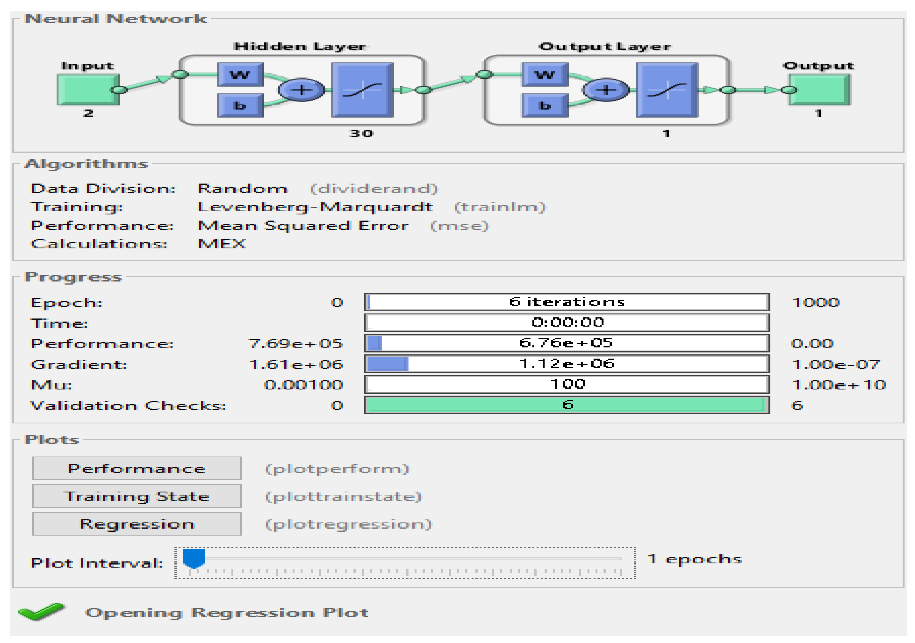
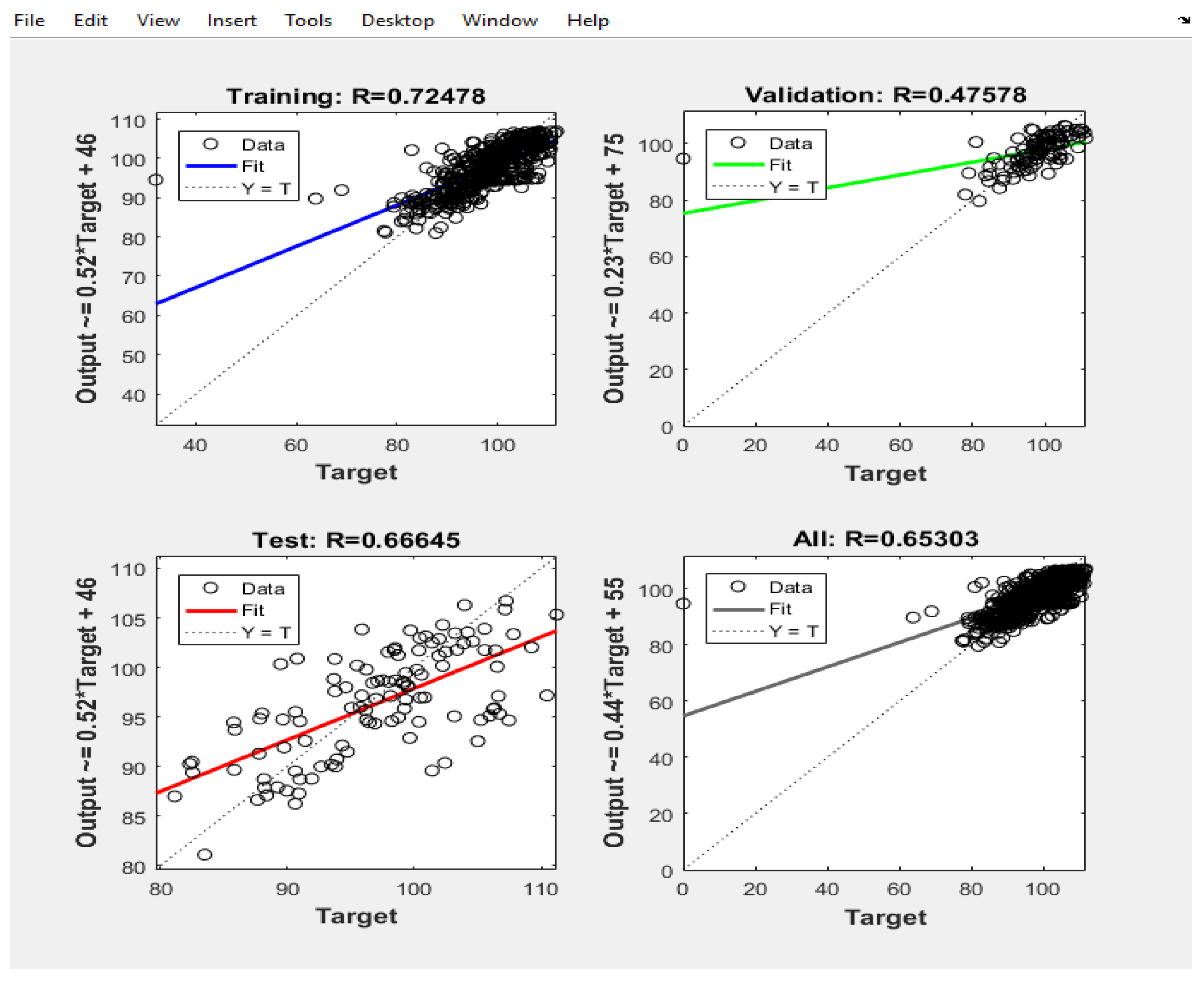
To determine the optimal network for the model, two separate networks have been constructed, each with n neurons in the hidden layer and one neuron in the output layer. Both the output layer and the hidden layer employ the tangent function. This configuration is illustrated in Figure2. This approach ensures that distinct networks are dedicated to predicting the number of hourly traffic and the average hourly speed, aligning with the researcher's view on the unique characteristics of each prediction task.
In
Table 1 and
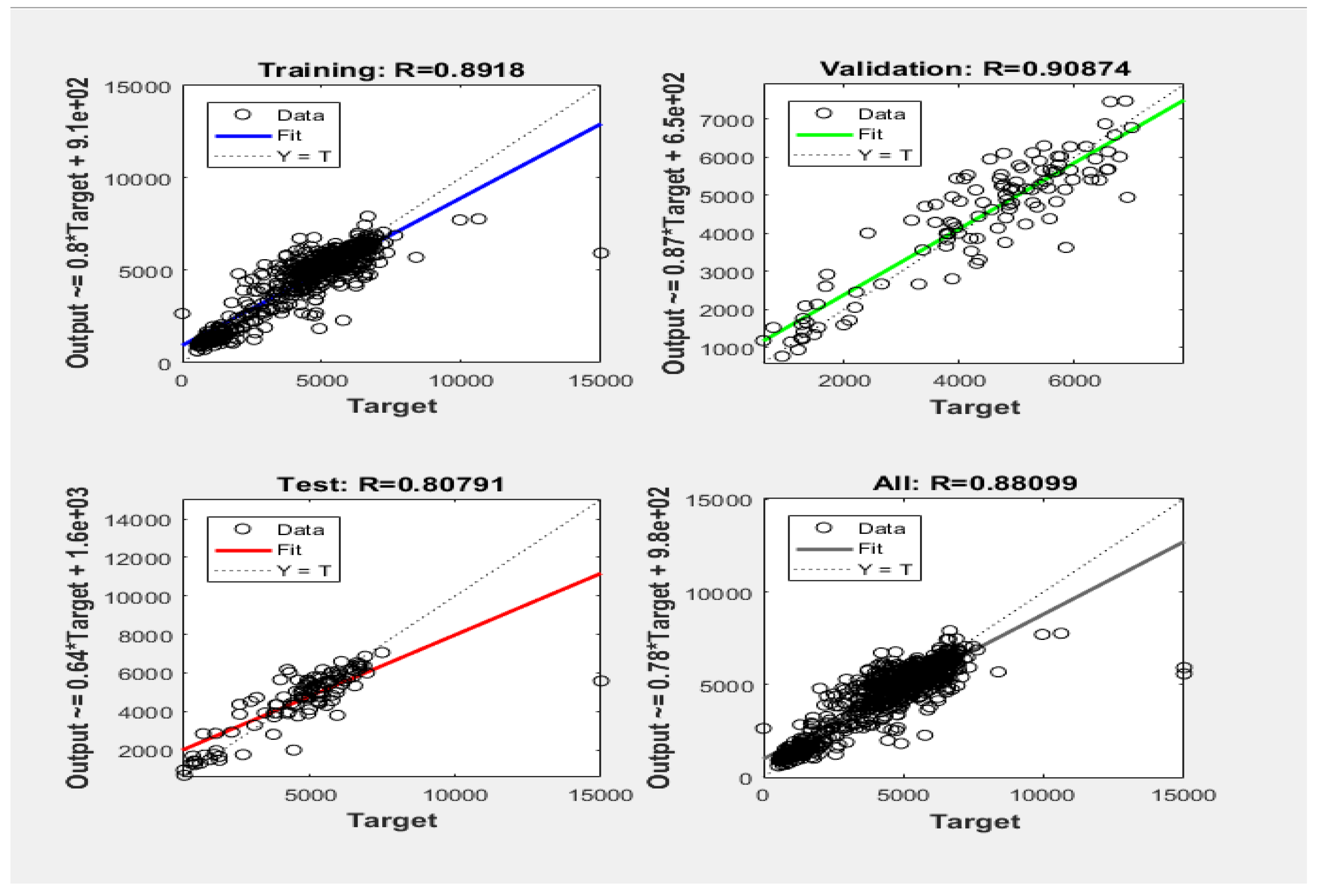
Figure 2 , the algorithm functions employed in the traffic volume neural network are detailed.
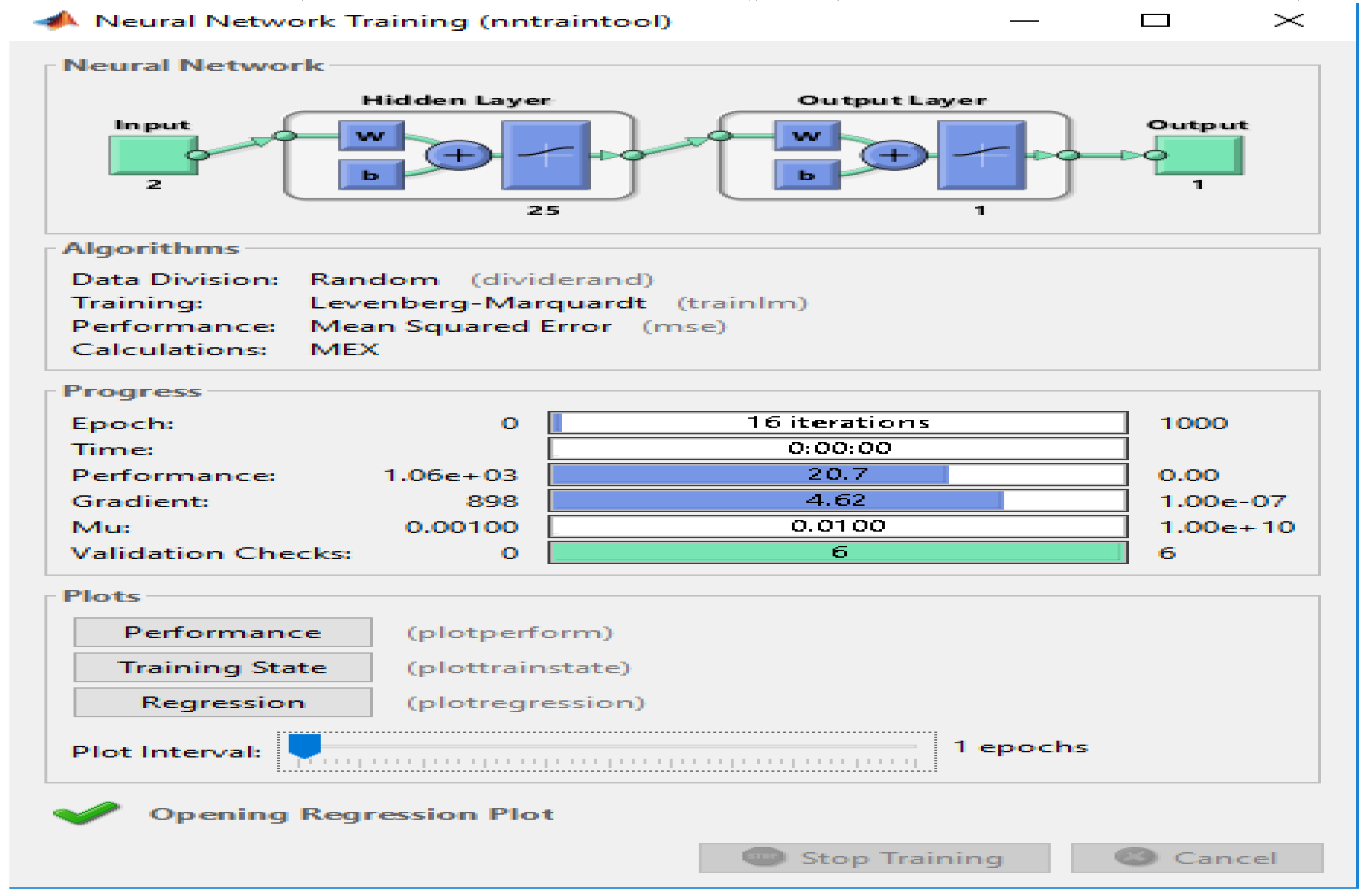
In
Figure 4 network for Speed the algorithm functions employed in the traffic volume neural network are detailed. For speed, a three-layer perceptron network with two input neurons and 25 neurons in the hidden layer and one neuron in the output layer has been used in the last layers.
5. Findings and Discussion
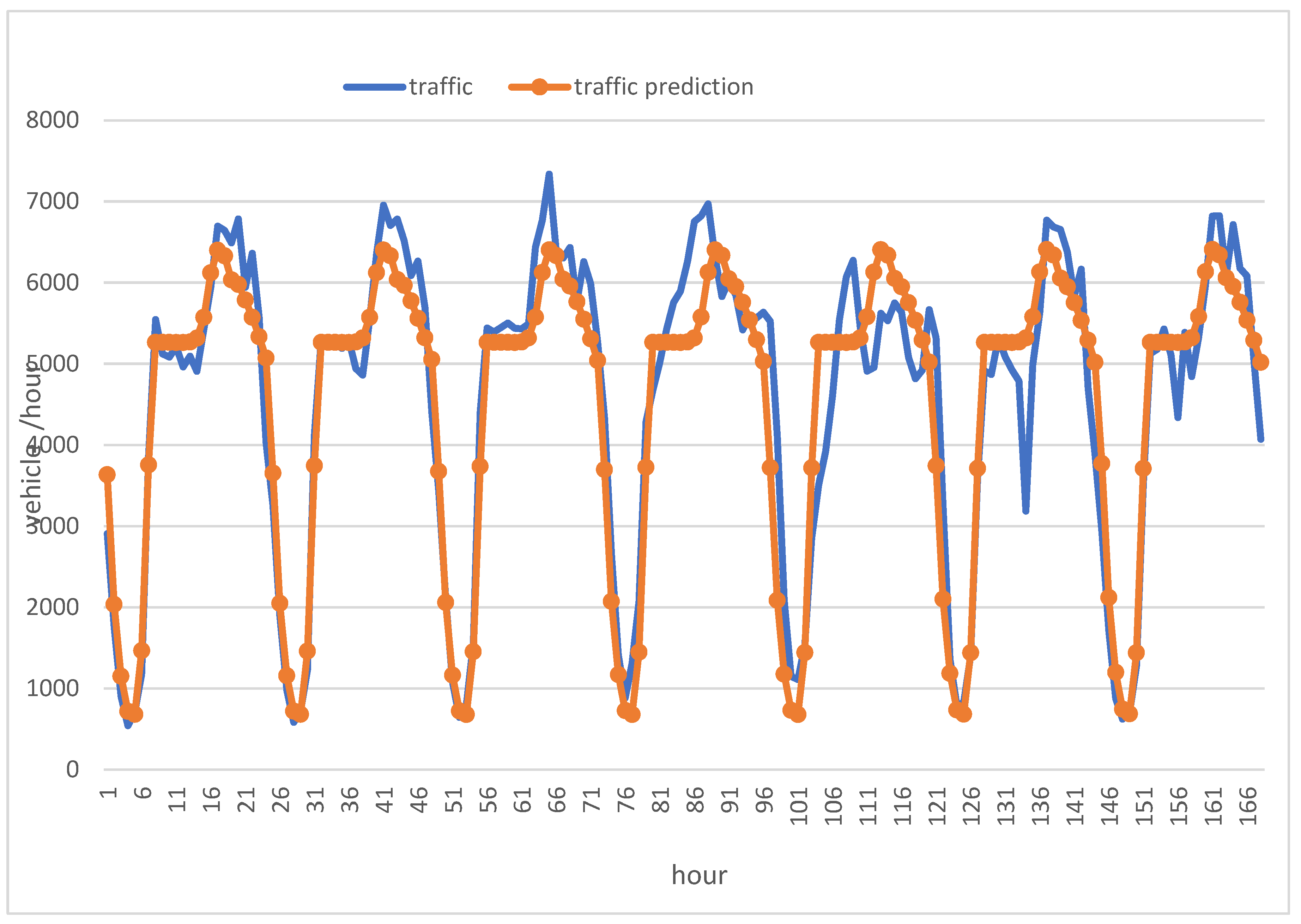
Table 3 displays the neural network output for the first week, organized into 168 rows. The initial column represents the day (1 to 7), followed by the hour (1 to 24). The "Average Speed" column showcases observed speed data, while the "Volume" column presents actual traffic volume from the counter. The last two columns, "Prediction Speed" and "Prediction Volume," depict the neural network's forecasts for speed and volume, respectively. This concise arrangement allows for a clear comparison between actual and predicted values, aiding in the assessment of the neural network's performance in forecasting both average speed and traffic volume over the specified time frame..
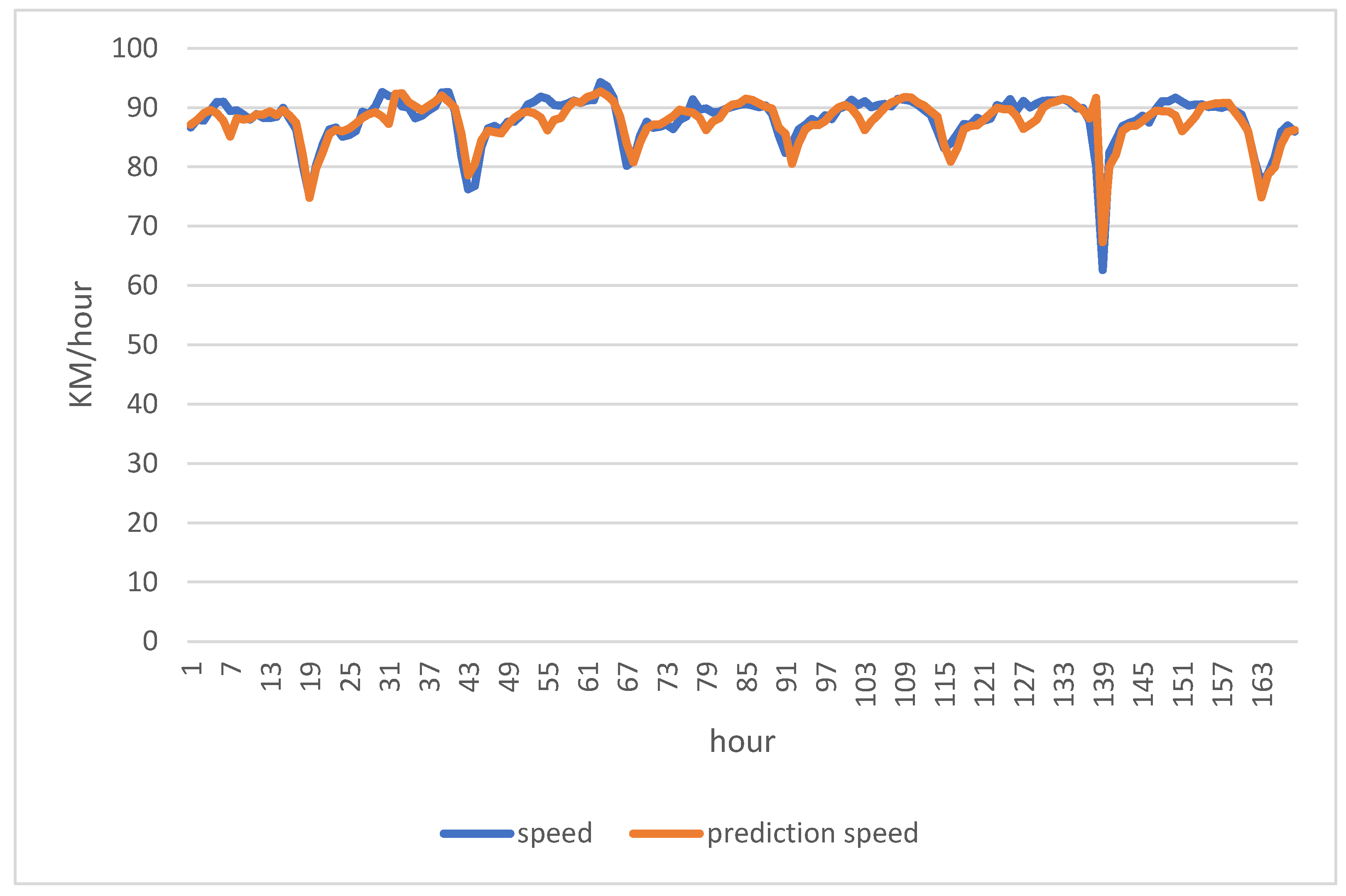
Mean Absolute Error (MAD) serves as a metric quantifying the average magnitude of prediction errors. For speed, the MAD is 4.15, indicating an average deviation of 4.15 kilometers per hour from the actual speed. In the case of traffic, the MAD is 822.87, signifying an average difference of 822.87 vehicles per hour between predicted and actual traffic volume. The Range, representing the spread between maximum and minimum values, is 29 for speed and 6321 for traffic. This implies that predicted speed spans from 25 to 54 kilometers per hour, and predicted traffic volume ranges from 1 to 6322 vehicles per hour.MAD/Range ratios offer additional insights. For speed, the MAD/Range is 14.30%, suggesting the average error constitutes 14.30% of the speed range. Similarly, for traffic, the MAD/Range is 13%, indicating that the average error constitutes 13% of the traffic volume range. These metrics provide a comprehensive understanding of the prediction accuracy relative to the variability within the dataset.
Figure 6 shows the number of vehicles per hour on a road over a period of time. The blue line represents the actual traffic, and the red line represents the predicted traffic. The green area represents the difference between the actual and predicted traffic.The traffic is highest in the morning and evening rush hours. The traffic is lower on weekends. The predicted traffic is generally accurate, but there are some discrepancies.
Figure 7 showing the predicted speed of traffic on a highway compared to the actual speed of traffic. The red line represents the predicted speed, the blue line represents the actual speed.
6. Conclusions
In conclusion, this study delved into the realm of traffic prediction, specifically employing the simple Multilayer Perceptron (MLP) model within the context of artificial intelligence. While various models exist for predicting traffic patterns, our investigation underscored the paramount importance of data quality over the intricacies of the model itself. Notably, the study revealed that data characterized by substantial error and fluctuation presented a more formidable challenge for accurate predictions.
Moreover, we argued for a nuanced approach to model evaluation, advocating against sole reliance on traditional criteria such as Mean Absolute Deviation (MAD) or coefficient of determination (r2). Instead, we proposed the utilization of MAD/Range as a more robust metric, particularly when confronted with datasets exhibiting significant order.The findings of this research, based on a set speed limit of 0.65 and a traffic value of 0.88, indicated parity in accuracy between predicting speed and traffic using the artificial intelligence model. Both criteria yielded MAD/R values of 13% and 14%, respectively, highlighting the model's consistent performance across different variables.
Ultimately, this study contributes to the evolving landscape of traffic prediction by emphasizing the need for a data-centric perspective and introducing an alternative metric for model evaluation. As transportation systems become increasingly complex, these insights pave the way for more effective and reliable predictions in the realm of traffic management.
Author Contributions
Conceptualization: Mohammad Maniat, Methodology, Software Writing—Amin Eebrahimzadeh:Writing—Review and Editing.
Data and Materials availability
Competing of interests
The authors declare that they have no competing interests.
References
- Wachs, M., The role of transportation in the social integration of the aged. The social and built environment in a older society. Washington, DC: Institute, 1988.
- Maniat, M., et al., The difference between the gentrification process in Latin America and other English-speaking countries (Case study Sã, o Paulo). 2023.
- Maniat, M., et al., The contrast of transit-oriented development, sustainable urban development and gentrification with a look at the cities of Karaj and Tehran. 2023.
- Akhtar, M. and S. Moridpour, A review of traffic congestion prediction using artificial intelligence. Journal of Advanced Transportation, 2021. 2021: p. 1-18. [CrossRef]
- Basheer, I.A. and M. Hajmeer, Artificial neural networks: fundamentals, computing, design, and application. Journal of microbiological methods, 2000. 43(1): p. 3-31. [CrossRef]
- Paola, J.D. and R.A. Schowengerdt, A review and analysis of backpropagation neural networks for classification of remotely-sensed multi-spectral imagery. International Journal of remote sensing, 1995. 16(16): p. 3033-3058. [CrossRef]
- Maniat, M., et al., Trip Distribution Modeling Using Neural Network and Direct Demand Model.
- Chen, X., et al., Sensing data supported traffic flow prediction via denoising schemes and ANN: A comparison. IEEE Sensors Journal, 2020. 20(23): p. 14317-14328. [CrossRef]
- Maniat, M., et al., Temporal and Spatial Correlation of Air Pollution with COVID-19 in the USA: Challenges and Implications. 2023.
- Sayed, S.A.; Abdel-Hamid, Y.; Hefny, H.A. Artificial intelligence-based traffic flow prediction: a comprehensive review. J. Electr. Syst. Inf. Technol. 2023, 10, 13. [Google Scholar] [CrossRef]
- Kumar, K., M. Parida, and V.K. Katiyar, Short term traffic flow prediction in heterogeneous condition using artificial neural network. Transport, 2015. 30(4): p. 397-405. [CrossRef]
- Çetiner, B.G., M. Sari, and O. Borat, A neural network based traffic-flow prediction model. Mathematical and Computational Applications, 2010. 15(2): p. 269-278. [CrossRef]
- Lu, S., et al., A combined method for short-term traffic flow prediction based on recurrent neural network. Alexandria Engineering Journal, 2021. 60(1): p. 87-94. [CrossRef]
- Olayode, I.O., et al., PREDICTION OF VEHICULAR TRAFFIC FLOW USING LEVENBERG-MARQUARDT ARTIFICIAL NEURAL NETWORK MODEL: ITALY ROAD TRANSPORTATION SYSTEM. Komunikácie, 2022. 24(2).
- Jia, T. and P. Yan, Predicting citywide road traffic flow using deep spatiotemporal neural networks. IEEE Transactions on Intelligent Transportation Systems, 2020. 22(5): p. 3101-3111. [CrossRef]
- Sharma, B., et al., ANN based short-term traffic flow forecasting in undivided two lane highway. Journal of Big Data, 2018. 5(1): p. 1-16. [CrossRef]
- Khair, U., et al. Forecasting error calculation with mean absolute deviation and mean absolute percentage error. in journal of physics: conference series. 2017. IOP Publishing. [CrossRef]
|
Disclaimer/Publisher’s Note: The statements, opinions and data contained in all publications are solely those of the individual author(s) and contributor(s) and not of MDPI and/or the editor(s). MDPI and/or the editor(s) disclaim responsibility for any injury to people or property resulting from any ideas, methods, instructions or products referred to in the content. |
© 2024 by the authors. Licensee MDPI, Basel, Switzerland. This article is an open access article distributed under the terms and conditions of the Creative Commons Attribution (CC BY) license (http://creativecommons.org/licenses/by/4.0/).
