1. Introduction
Automated vehicle controllability in any scenario especially in emergency situations plays a key role in the safety system design. Public acceptance [
20,
26,
27] is another important factor that improves with the capabilities of the safety systems. More and more intelligent safety mechanisms need to be part of the automated vehicles to mitigate this risk in the future and cover all types of scenarios in a proactive and distinguishable way. Operational Design Domain (ODD) [
9,
12,
13] has become increasingly important for Level 2, 3 and 4 automated vehicles [
5] because their performance is usually judged based on the in-scope elements for ODD. For example, if the current ODD is only to handle Urban driving upto 45 mph, then the capabilities of the system would be defined to cover all the scenarios that the vehicle encounters in this particular ODD. The system architecture would be designed with this short-term goal in mind along with the future potential of expansion in the scope. The sensor detection ranges [
28,
29,
30] are estimated based on this definition to be able to handle the scenarios involving operation upto 45 mph like being able to detect traffic lights for example. Similarly, the safety case [
15,
31,
32] would include safety goals, safe state mechanisms that cover the in-scope scenarios in detail. The safety case also has another aspect of handling out-of-scope elements, which involves critical thinking and understanding the operational limitations of the system. Operational limitations on the actuators have been studied before but how to make these thresholds more dynamic and flexible based on the ODD and scenario parameters as they evolve over time and as we move towards higher levels of autonomy has not been considered enough. There is a need for making this limits application strategy more intelligent and adaptable over time. The transition from traditional vehicle dynamic safety limit tables to environmental and scenario based safety limits generated online based on the environment and scenario parameters offers several benefits:
Adaptability to Real-Time Conditions: Environmental-based safety limits are dynamically generated in real-time, considering the current environmental conditions. This adaptability allows for more accurate and context-sensitive responses, as opposed to static tables that may not account for the variability in real-world driving scenarios.
Increased Safety: By considering factors such as weather, road conditions, traffic density, and pedestrian activity, these dynamic limits can enhance safety. They allow the vehicle to adjust its behavior in response to immediate surroundings, reducing the risk of accidents due to unforeseen environmental factors.
Efficiency and Performance: Dynamic limits can optimize vehicle performance by adjusting to the environment, ensuring that the vehicle operates efficiently under varying conditions. This can lead to better fuel efficiency, reduced wear and tear, and an overall smoother driving experience.
Scalability and Learning: As driving environments evolve, traditional tables can become outdated. Dynamic limits, however, can evolve with the environment, continually improving and adapting to new conditions.
Addition of Decision Making (DM) capabilties is needed to make this transition and adaptability possible. Decision Making (DM) Engines using Multi-Criteria Decision Making (MCDM), Decision Trees and Random Forest helped solve numerous problems and has evolved over time to be data-driven [
2] as more and more data is made available. Decision Making (DM) Engines are the systems that are designed to facilitate the Decision Making (DM) algorithms or processes required. Decision Making (DM) algorithm is a step-by-step set of instructions or a computational procedure designed to solve a specific problem. Operational limitations of the system are being addressed in this paper with various examples as mentioned in the
Section 4. The ODD definition helped to further define and decompose the system behavior that is needed to be developed. Scenarios that are in-scope have been derived from the detailed ODD elements as mentioned in section 5 of the AVSC best practices [
12] which in-turn helped with defining the required capabilities and a set of system behaviors.
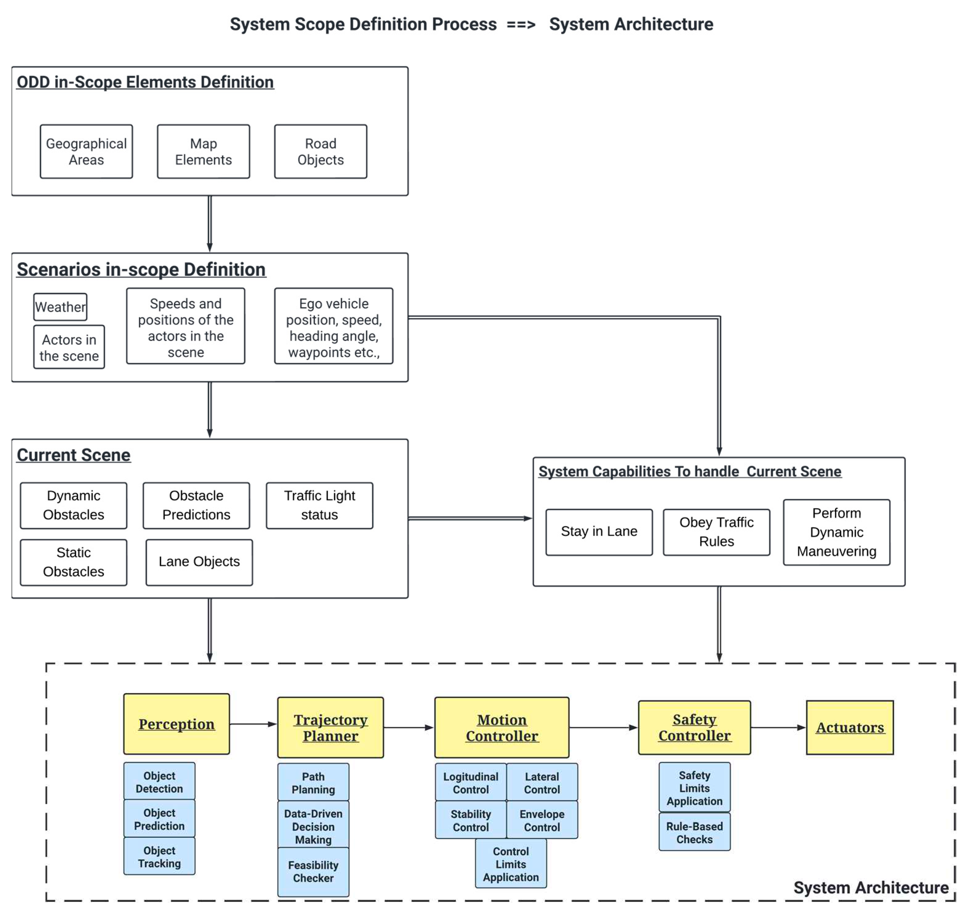
Figure 1 illustrates the complete workflow of defining the system behaviors starting from the ODD definition until the application of controls and safety limits [
1] within the actuators.
Leveraging a simple version of these DM algorithms in all aspects of safety but with proper supervision and safety principles [
11] makes the new approach more powerful and valuable. One good example of such algorithm has been discussed in
Section 5 of this paper. This algorithm takes in the required driving scenario parameters [
14] and outputs the classification of safety limits to be chosen to achieve a certain type of trajectory customized for each scenario.
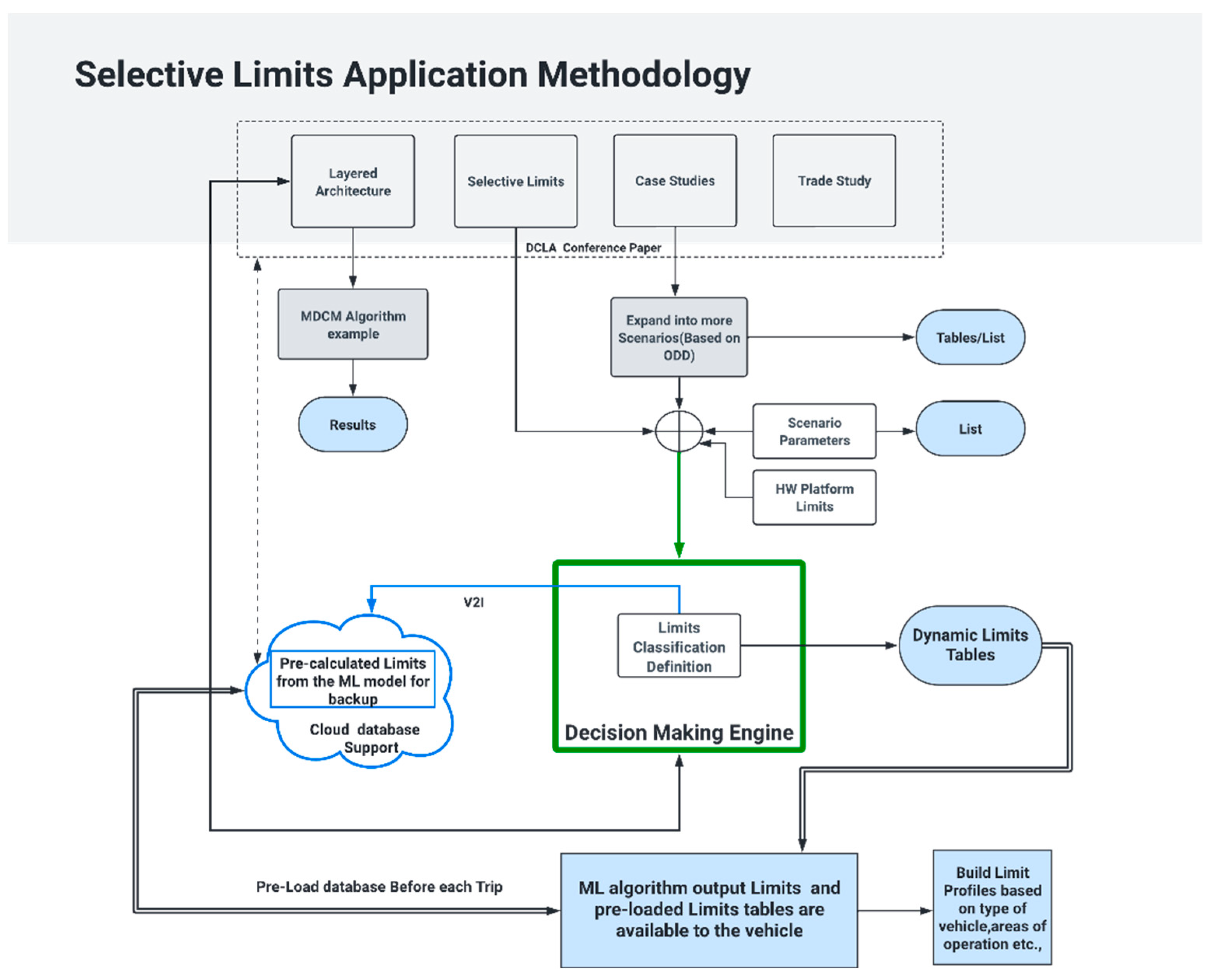
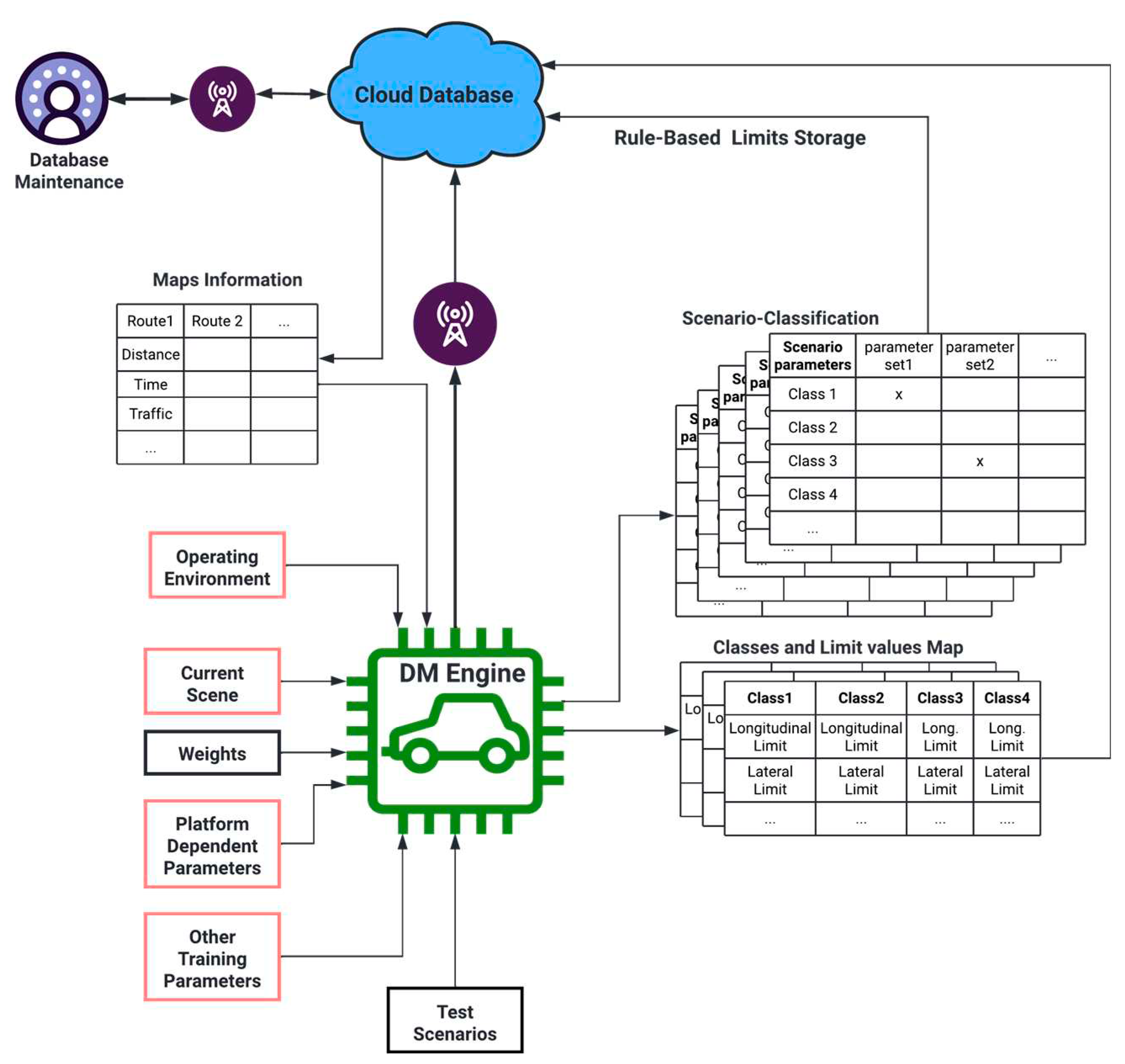
Figure 2 below covers all the extensions from the DCLA strategy [
4] that this paper addresses like incorporating the concepts of system definition process, ODD definitions along with using Decision Making (DM) Engine, providing the complete methodology for selecting the right classification of limits in each of the driving scenarios while also leveraging the cloud database network or the V2I [
3] capability to reduce the on-board processing and storage needed for the components in-vehicle during nominal and failure scenarios of certain algorithms.
2. Limits Evolution and Scenario Identification
Dynamic limits ensure safe vehicle maneuvering in automated driving. The safety controller sets constraints based on the vehicle state, such as current speed, and determines controlled commands or limits. If the actual controller command surpasses the determined limit, the safety controller’s limiter logic is activated, adjusting the output value accordingly. This process, already in use in automated vehicles [
33,
35], prevents exceeding safety thresholds, such as limiting steering angle values that could lead to disengagement if surpassed. In the case of applying steering angle rate limits, predefined limit values based on vehicle speed [
43] are commonly hardcoded into the software, limiting flexibility across various scenarios. However, a more adaptive approach involves developing multiple tables dynamically selected based on the scenario, allowing greater customization during vehicle operation. A model predictive controller (MPC) [
42] can then use these dynamic safety limit tables as constraints, ensuring controller commands align with established safety limits. The Decision Making (DM) Engine plays a crucial role in reliably detecting and classifying scenarios, applying the relevant set of limits. The DM algorithm dynamically adapts during automated vehicle operation, identifying and categorizing new scenarios. When a novel scenario is detected, it is sent to a cloud database using V2I [
3], where it is mapped to an existing class of limits based on DM-extracted parameters and saved for future reference as shown in
Figure 3. In the cases, where the newly identified scenario doesn’t fit into existing classes, the DM algorithm signals this, and V2I-equipped vehicle systems notify the cloud database. Periodic checks by database maintainers ensure updates for new scenario classes. While our work currently focuses on four classes, this can adapt to evolving scenarios. This approach ensures the cloud database evolves with expanding Operational Design Domains (ODDs) and exploration of new aspects, reducing on-board storage needs, but comes with a caveat of the vehicles always needing to have continuous connectivity to the cloud infrastructure. To eliminate this shortcoming, the cloud database is only being used for storing all the mappings of
"Scenario Classes <=
> Limits Tables" that were already taken from the outputs of the DM algorithms in known scenarios previously as shown in
Figure 3. Pre-loading the limits cloud database along with maps information within the vehicle before starting the trip is going to make this available to the system. This serves as a solution in case of network failures as well.
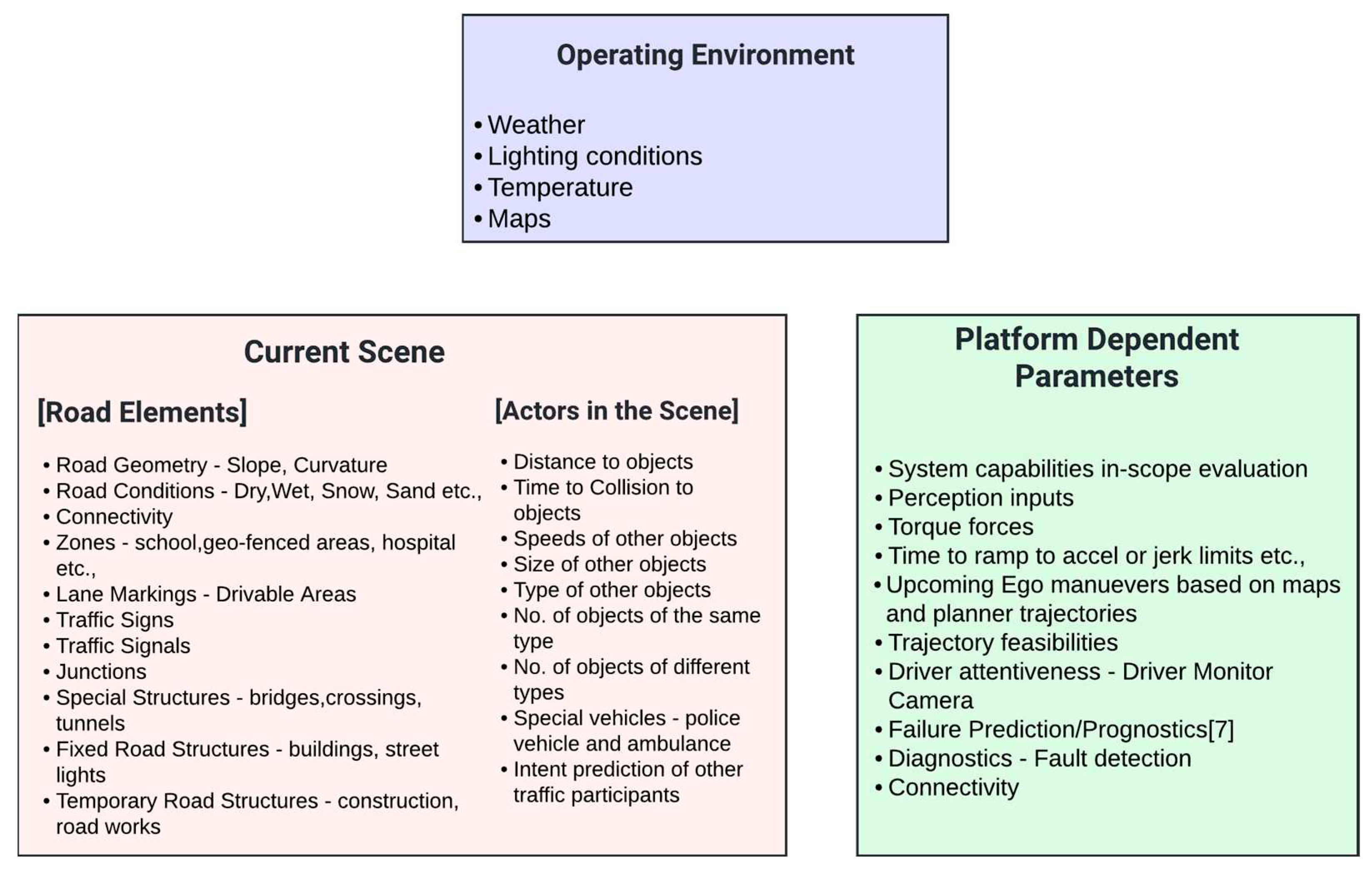
To utilize a DM algorithm, identifying the parameters and tuning hyper parameters is crucial. These parameters encompass operating environment factors (weather, lighting, connectivity), current scene details (road geometry, conditions, markings, signs, structures, actors, ego vehicle parameters), and platform-dependent parameters (ego vehicle system capabilities and physical limitations) as shown in
Figure 4. These considerations, coupled with criticality metrics, such as trajectory, maneuver, energy, uncertainty, or their combinations, contribute to effective DM algorithm performance, as highlighted by Cai et al. [
17].
3. Limits Classification
The autonomy system’s primary functions at different layers can be explained in simple steps as follows and has been illustrated in
Figure 1:
Step1: Perception detects, predicts and tracks the changes in the first 2 categories of scenario inputs mentioned above in
Figure 4. [
At certain Accuracy and Reliability levels].
Step2: Planner [
10] based on current data, previous data, previously followed behav- iors and checking the intended behaviors against traffic rules and violations determines a set of feasible trajectories.
Step2.1: Feasibility checker algorithm within the Planner considers the 3 categories of inputs like the perception inputs, environmental conditions and in-vehicle parameters to pick and choose the limits to be applied and picks the most feasible and appropriate trajectory - [
This is the algorithm that is being further expanded to add more DM capabilities and the cloud database support in this paper to create limits tables and choose the limits dynamically.]
Step3: This is in turn updated in the limits database on the cloud using V2I [
3]. This limits database acts as a ground truth in the known scenarios, backup in some extreme cases and failure cases where the DM Engine’s capabilities are limited. Some corner cases [
17] scenario limits or tables are created as well before-hand to provide more coverage.
Step4: Controller [
21,
34] follows the most feasible and appropriate trajectory selected by the planner, by applying the limits that were chosen by the Feasibility checker algorithm.
Step5: Safety Controller checks if there are limits applied and if they are within the safe operational boundaries. If not, a pre-coded set of limits will be applied. [These limits are present on-board the vehicle that are pre-loaded using the cloud database from Step4.]
The feasibility checker algorithm in Step 3, illustrated in
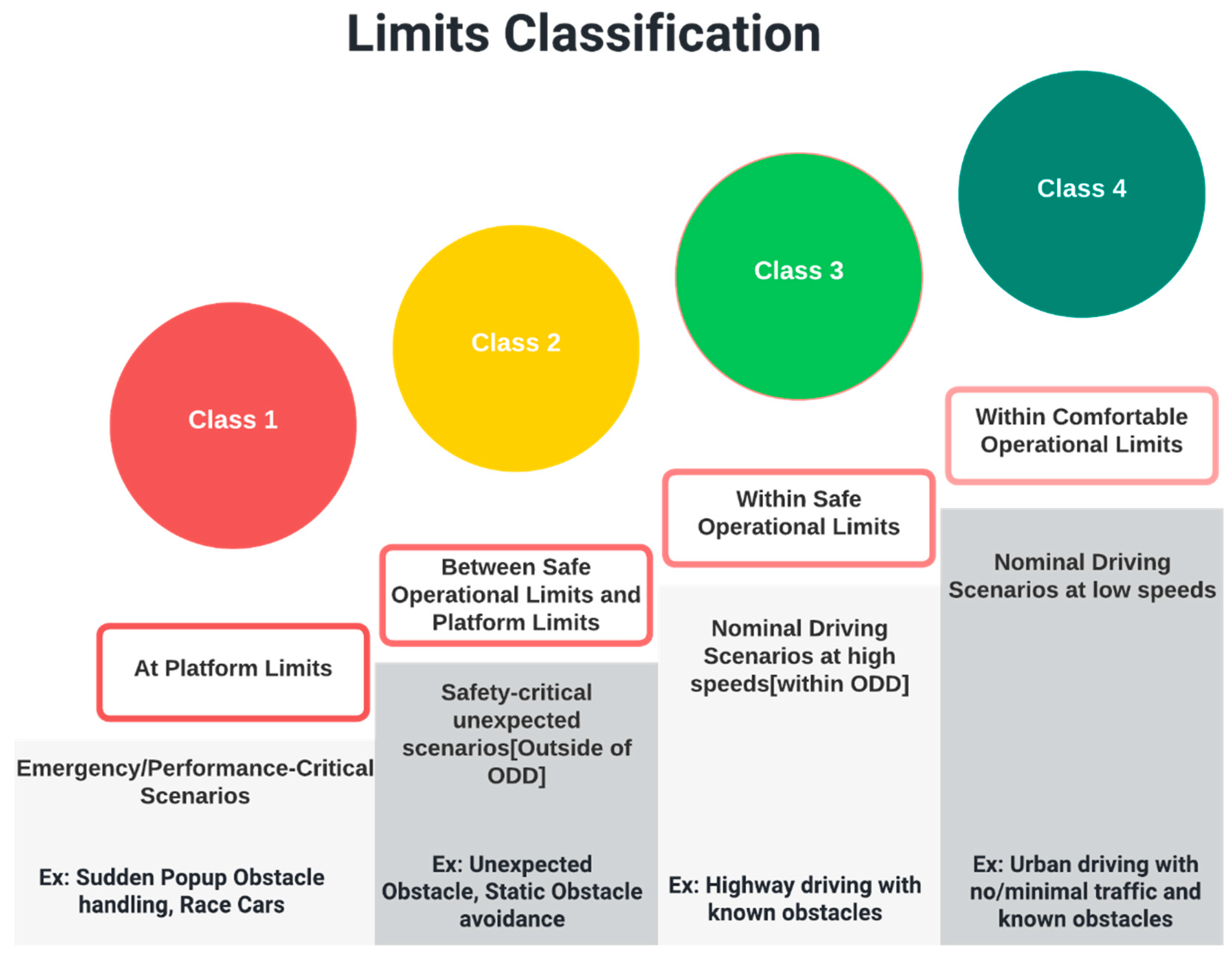
Figure 4, will incorporate DM algorithms to automatically select appropriate limits for each scenario. The ML algorithm classifies scenarios into four distinct classes based on input parameters. Focusing on longitudinal and lateral control limits,
Figure 5 depicts a clear classification of limits according to scenario severity and risk level. Three types of limits—platform, safety, and comfort—are applicable in all scenarios and further divided across the four classes:
Class 1: For this class, being at the highest severity and risk level [
36], the maximum limits that the vehicle platform can allow needs to be applied. There are cases where the component designs can be altered as well to apply limits exceeding the current physical limitations [
23]. Most of the critical scenarios [
25] fall into this category.
Class 2: This class is still at a high risk and severity level but less than Class1. Choosing the limits that are within the platform limits but more than a normal safe operational limits would be necessary [
22,
24].
Class 3: This class covers the most common scenarios that are seen during normal driving but high speed or other slightly elevated risk level conditions are associated with it. Choosing the limits that are within the safe operational constraints would be sufficient in this case.
Class 4: This class consists of all the normal driving scenarios with minimum possible risk level involved and applying the comfort limits is usually sufficient
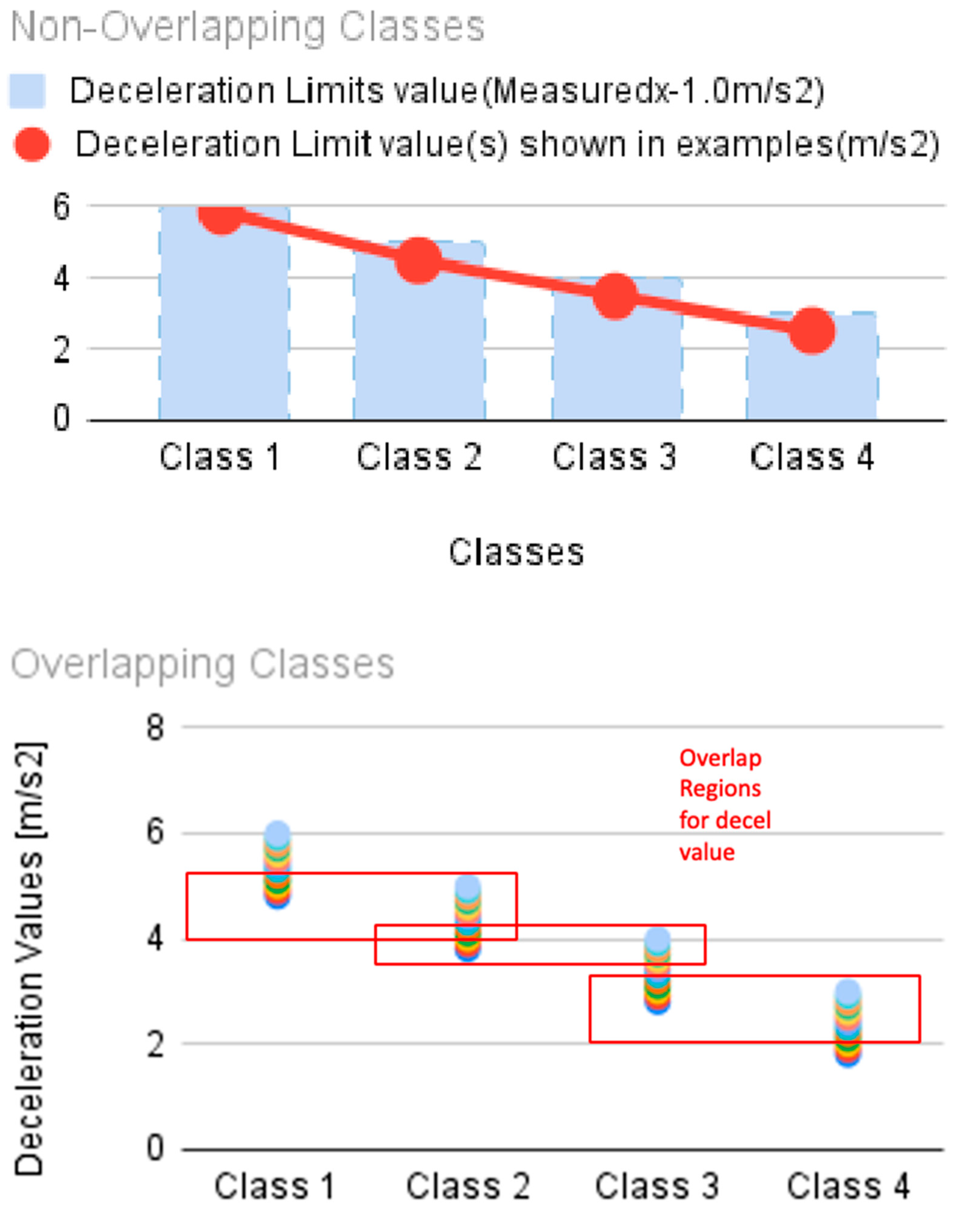
While these classes are defined distinctly, there may be overlap in limit values based on operating scenarios. For instance, the least comfortable longitudinal limit in Class 4 could be the same as the best-case scenario within Class 3, indicating potential correlations between classes as shown in Figure 13.
Figure 5.
Limits Classification.
Figure 5.
Limits Classification.
4. Scenario Case Studies
Diverse case studies have been conducted using 2 different vehicle platforms to make sure that the classification of scenarios applies independent of the platform being tested. First vehicle platform is a full autonomy intent platform that was purpose built to scale to Level 5 Autonomy in the future. Second vehicle platform is an automated driving platform that was custom built to have Dual-Cockpit design for specific research use cases in terms of Advanced Driver Assistant Systems and Parallel Autonomy [
15,
46]. These 2 vehicle platforms were tested in various scenarios and environments like closed courses and public roads which provided insights into the distinct ranges of limits values applicable to each scenario class. As the scenario set could be very large to reach an accurate conclusion, we had to restrict the case studies to certain known critical scenarios like strong emergency braking, sharp turns, J-turn etc., which provided enough insights on the value ranges of the limits needed for each scenario class. One example selection of these ranges has been presented in this section based on the case studies, extensive working knowledge on similar case studies along with a projection of the results to other scenarios that already fall into one of the 4 classes presented in
Section 3.
4.1. Longitudinal Limits:
Figure 6.
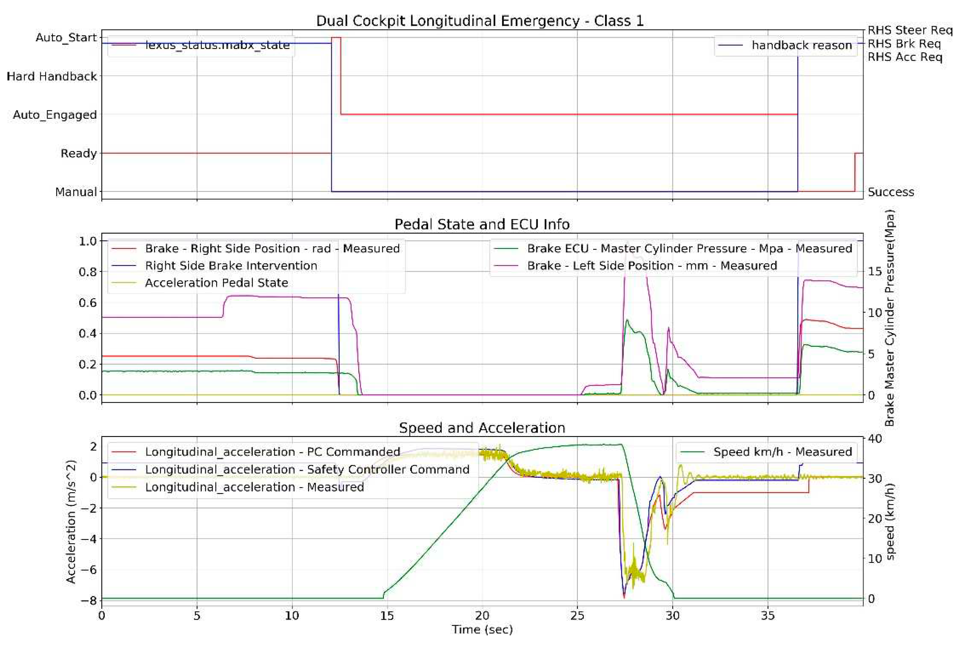
Strong Emergency Braking.
Figure 6.
Strong Emergency Braking.
Results Discussion: The first subplot indicates the state of operation of the system like man- ual, hand back or autonomy. The second subplot shows the brake master cylinder pressure, if there was a brake intervention from the human, and the brake pedal position. Finally, the third subplot illustrates the deceleration profile of the system with the commanded, measured and the safety controller acceleration and deceleration values. At time instance 18-22 secs, the acceleration value of 1.7 m/s2 has been reached. At time instance 26-28 secs, the deceleration value of 0.6g has been reached. Also, the measured values follow the commanded values as expected. Conclusion: Deceleration Class1 example scenario at 5.88 m/s2 and an Acceleration Class 2 example scenario at 1.7 m/s2 have been identified.
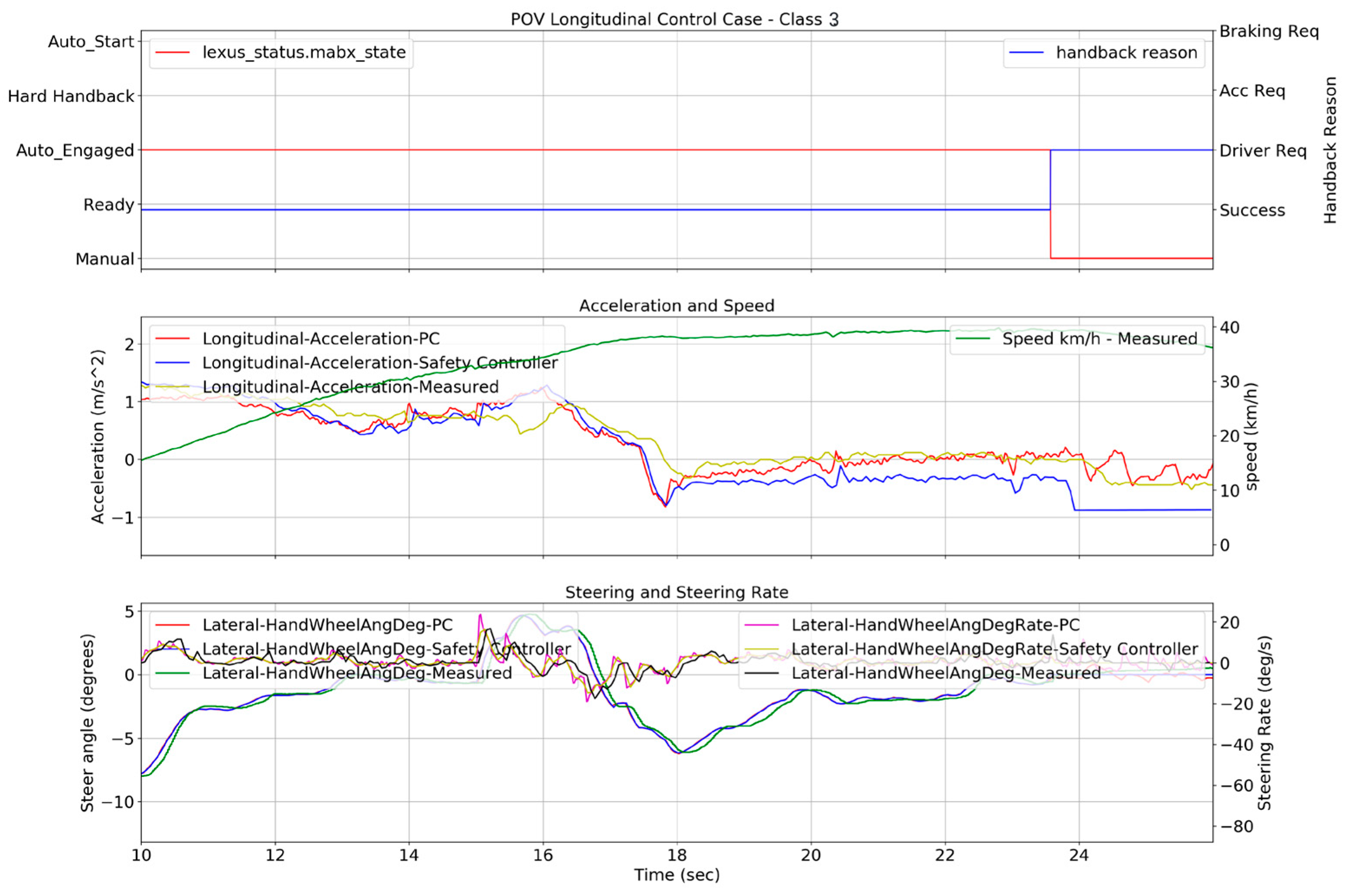
Results Discussion: The maximum acceleration applied in this case did not exceed the range of 1-1.5 m/s2 acceleration. To be able to maintain the controllability of the vehicle in terms of getting closer to the bicyclist. Conclusion: Acceleration Class 3 at >1.5 m/s2 scenario has been identified.
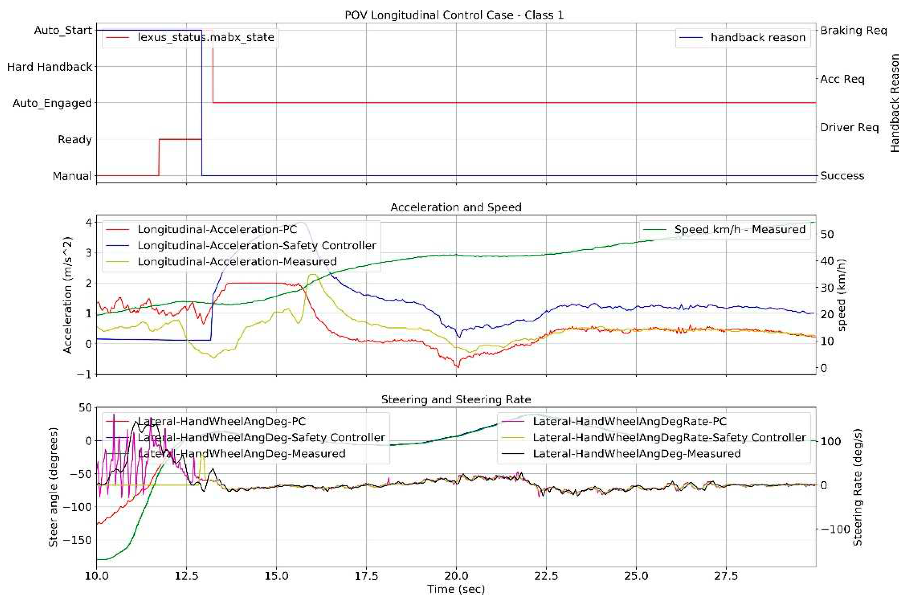
Results Discussion: Between 15 - 17.5 secs, the acceleration value exceeded 2.0m/s2 which could be classified as the Acceleration Class1 value and then it follows nominal acceleration values of 0.7 to 0.0 m/s2 between 17.5 -20 secs which falls into the Class 4. Between 20-21 secs, nominal deceleration value of 0.2 m/s2 has been observed which falls into the Class 4 deceleration values category. Conclusion: Acceleration Class 1 and 4 along with Deceleration Class 4 scenarios have been identified.
Figure 7.
Driving near a Bicyclist.
Figure 7.
Driving near a Bicyclist.
Figure 8.
Start From Stop.
Figure 8.
Start From Stop.
4.2. Lateral Limits:
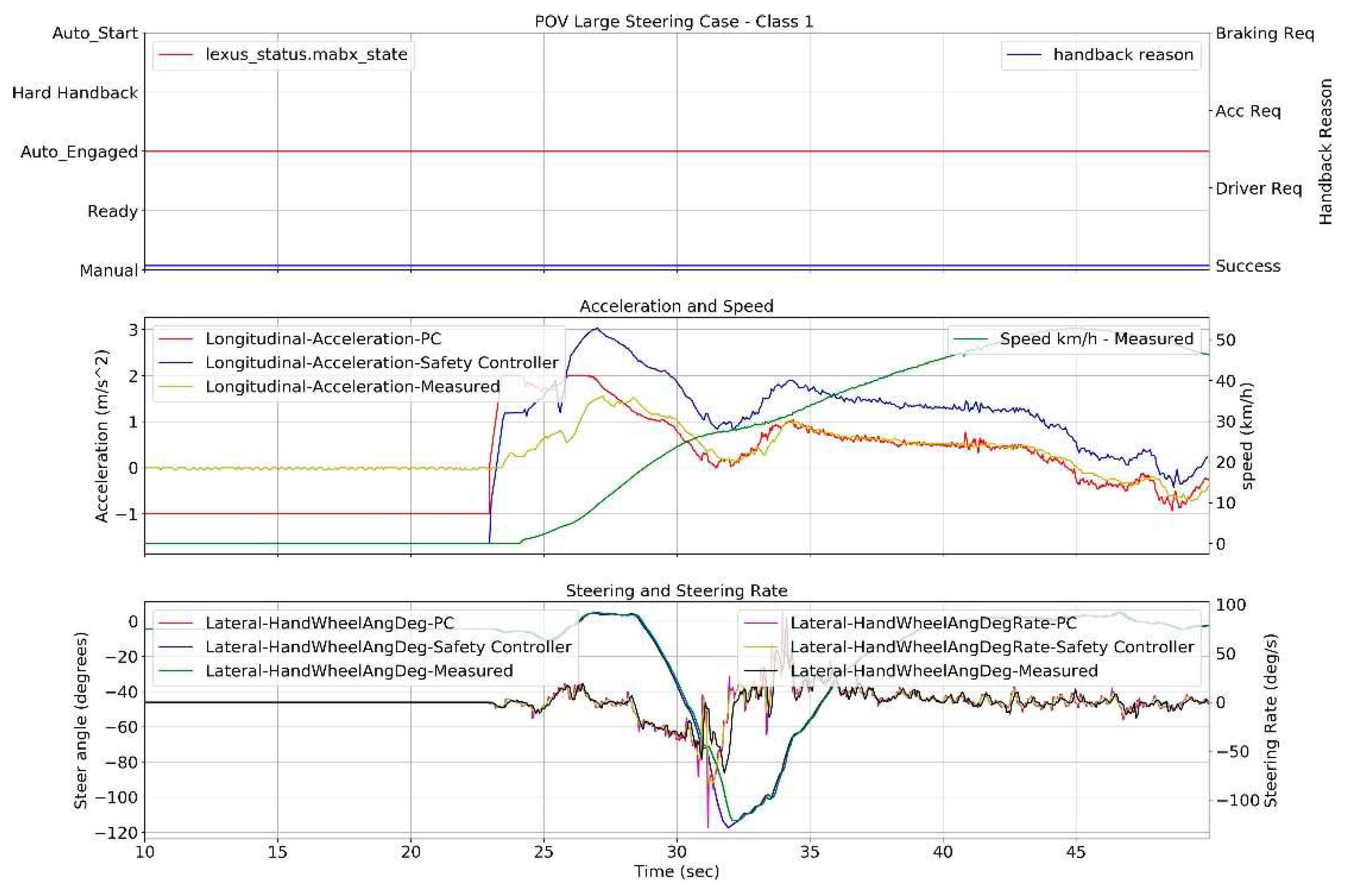
Results Discussion: Between 30 - 35 secs, there is a large steering angle between 100-120 deg which falls into the Class 1 steering angle values. At 32 secs, there is a large steering angle rate of 80 deg/sec which falls into the Class 3 of the steering angle rate. Conclusion: Steering angle Class1 and steering angle rate Class 3 scenarios have been identified.
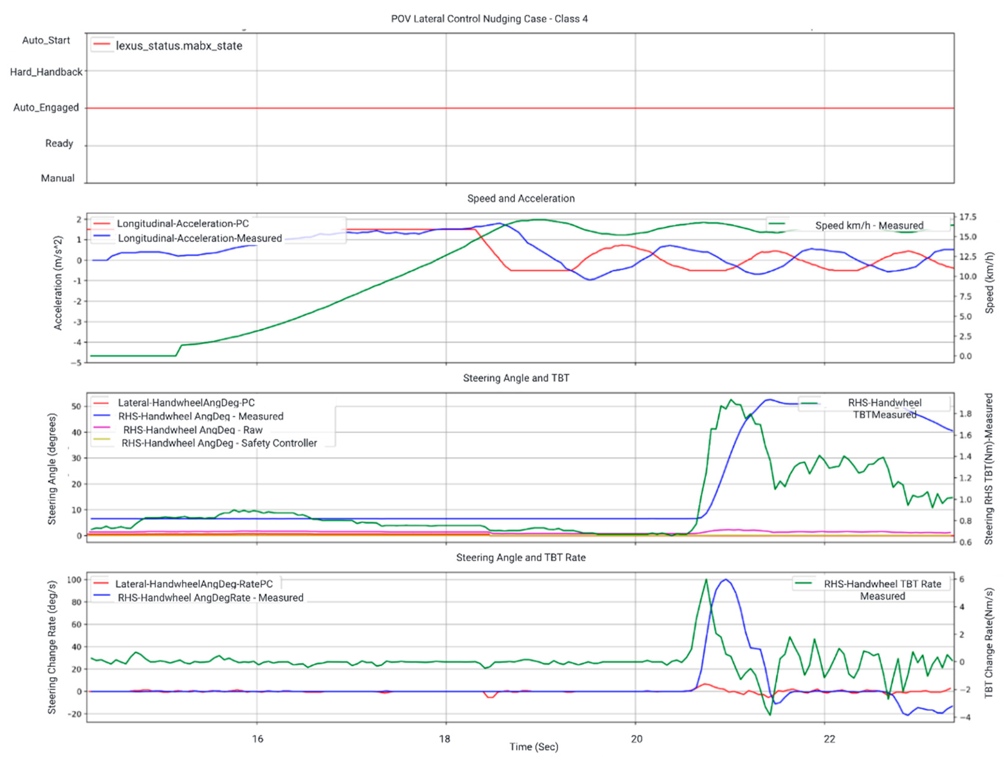
Results Discussion: This is a drive-by-wire system example and we have two steering angles i.e a Dual-Cockpit vehicle. The 2nd subplot plot: blue line is the measured steering angle from the hand wheel which reflects the driver’s input. The purple line is the calculated steering angle from the road wheel, which means the AV stack’s input. The 3rd plot: blue line is the measured steering angle rate from the hand wheel, which reflects the driver’s input. The red line is the calculated steering angle from the road wheel, which means the AV stack’s input.The blue line and red line are not necessarily matching, because of the the driver’s input. We see that the blue line in the 2nd subplot represents a small steering angle around 8 deg to the left being applied for nudging between 14-20 secs. Conclusion: Steering angle Class4 scenario has been identified.
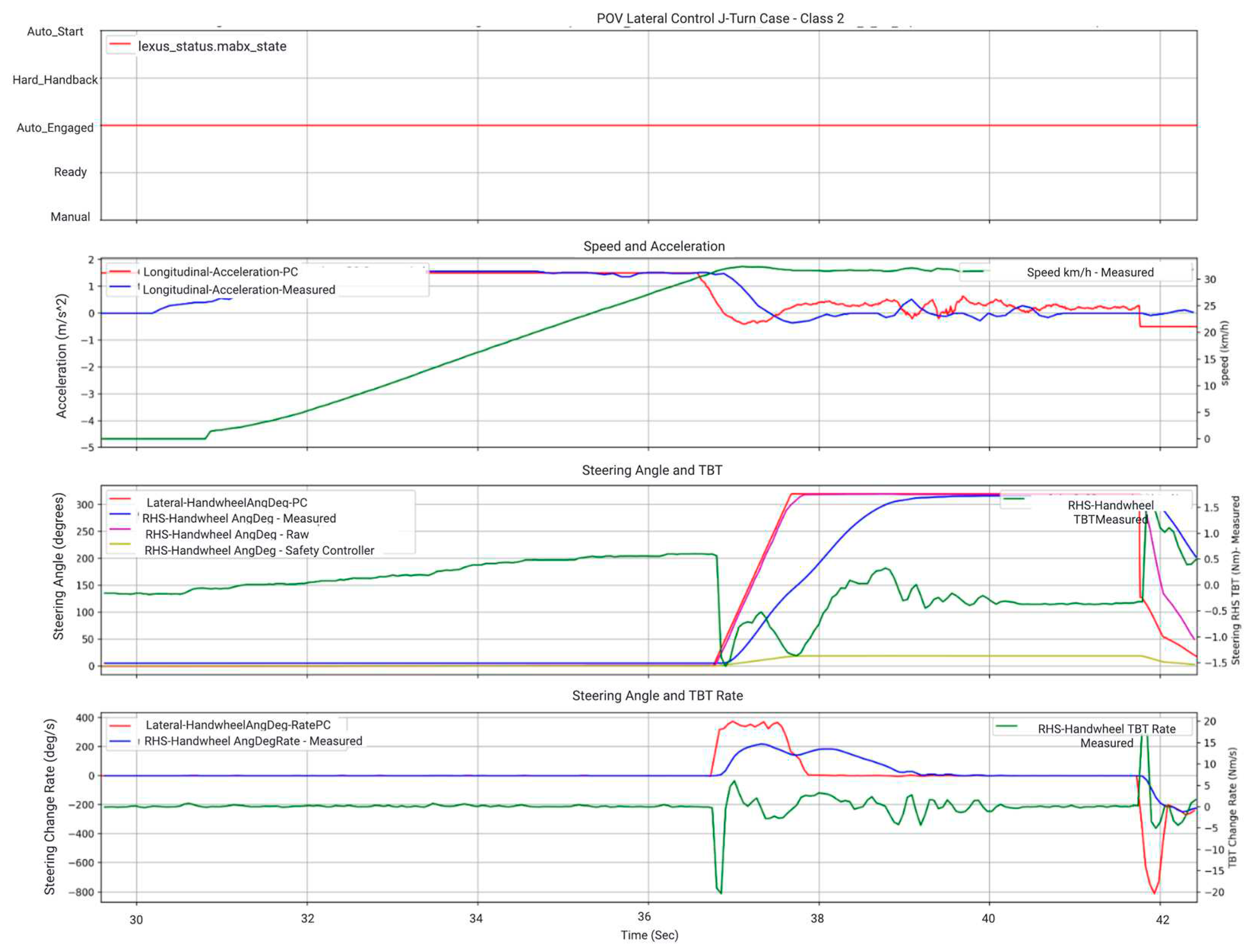
Results Discussion: On the 2nd subplot, red line indicates the steering angle commanded from the PC.Between 37-43 secs, the steering angle commanded >300 deg to be able to complete the J-turn maneuver at 20kmph. Conclusion: Steering angle Class2 scenario has been identified.(Note:Based on lower speeds like 20kmph, the limit for Class2 would be <350 deg)
Figure 10.
Nudging Scenario.
Figure 10.
Nudging Scenario.
4.3. More Class Examples:
Class 1:[Emergency Cases]
As per Funke J. et. al [
7] emergency scenarios demand vehicle maneuvers at operational limits to prevent collisions and maintain stability.
Extreme cases, such as race car driving, exemplify system models operating at friction limits.
Longitudinal critical scenarios include rapid acceleration from a stop or reaching a specific speed promptly.
Lateral critical scenarios involve U-turn steering and swerving to avoid sudden obstacles.
Operating at or above friction limits on icy/snowy roads is another example in this class.
Class 2:[Warning Cases]
Longitudinal: Braking for Lead Vehicle, Worst-case scenario considers a suddenly stopped lead vehicle scenario.
Lateral: Nudging over parked cars, U-turn scenarios etc.,
Class 3:[Elevated Caution]
Longitudinal :Coming to a stop at the Traffic lights stop line, Normal braking for lead vehicle scenarios etc.,
Lateral : Taking Right Turns at the Traffic Lights at lower speeds.
Class 4:[Nominal]
Longitudinal: Low speed urban driving with less traffic, normal braking for speed adjustments during low speed driving.
Lateral: Normal steering or no steering required scenarios.
Based on scenario case studies, prior working knowledge, and examples provided earlier,
Table 1 and
Table 2 summarize chosen limit values for longitudinal and lateral limits, respectively.
Table 3 provides an example of deceleration limit classification based on scenario inputs like the current scene, weather conditions and platform dependent parameters as was introduced in
Section 2. Finally,
Figure 13 illustrates the behavior of limit values when transitioning between classes, presenting variations of overlapping and non-overlapping classes.
5. DM Algorithm Case Study
As we have now derived the limits tables and their mapping towards the classes
(Scenario Classes<=
>Limits Tables) already in
Section 4. This section provides a case study on how to apply a Decision Making algorithm using the Feasibility Checker within the Planner as defined in
Section 3 in Step 2.1 to determine the
"Classes" of the driving scenarios. For this case study, Multi-Criteria Decision Making(MCDM) algorithm [
44] is being considered. MCDM is more suitable for complex decision problems with multiple conflicting criteria. It is highly flexible, offers clear interpretation of criteria weights and alternatives’ performance. MCDM is really good at handling uncertainty through sensitivity analysis and scenario analysis. There are multiple types of MCDM algorithms [
44] like WSM, AHP, WPM and TOPSIS [
45]. TOPSIS algorithm has been chosen for our case study as it is relatively simple, easy to understand and can be easily adapted to different decision making scenarios by adjusting criteria and their weights. We considered one example scenario of
"Driving in Rain" and created a synthetic randomly generated dataset as shown in
Table 4 that consisted of 1000 different scenarios with multiple variations of parameters like Rain level, Time to Collision (TTC) to other objects in the current scene, Ego vehicle speed in the current scene and the road surface friction. The Rainfall rates have been taken from the AVSC ODD Framework [
12] i.e., Light rain: Less than 0.1 in/h, Moderate rain: 0.1 to 0.3 in/h, Heavy rain: 0.3 to 2.0 in/h and Very heavy rain: More than 2.0 in/h. Ego vehicle speeds have been considered between 5 and 85 mph which covers a wide range of speeds. Friction values for Dry Asphalt or Concrete (0.7 to 0.9), Wet Asphalt or Concrete (0.4 to 0.7) and other low friction values have been considered upto a value of 0.0. For the ease ofTOPSIS application, we have used equal weights for all parameters to start with.
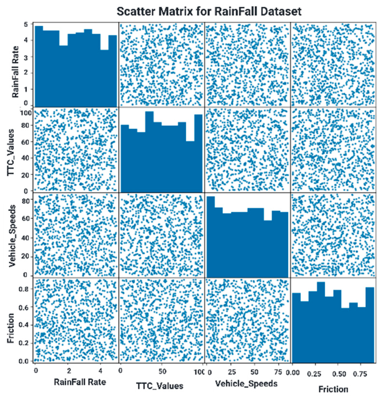
The diagonal cells in
Figure 14 contain histograms that represent the distribution of values for each variable. Histograms display the frequency or count of data points within specific bins or intervals. The shape of the histogram provides insights into the distribution of a single variable. This is important in exploratory data analysis (EDA) to identify patterns and potential issues with individual variables. In the scatterplot matrix’s off-diagonal cells, each point represents a data point, with its position on the x and y axes corresponding to values of the two variables being compared. Random scattering of points suggests a weak or no correlation between the variables and hence with the scenario set being considered.
5.1. TOPSIS Algorithm:
The generated dataset has been considered as the matrix X with n scenario variations with m criteria. First step is to normalize each criteria and then assign the weights to each criteria.
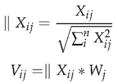
Then, determine the ideal

and

non-ideal values
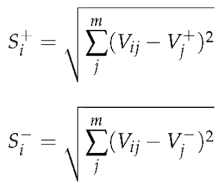
for each criteria from the previously normalized and weighted values. These values are then used to calculate the Euclidean distances to each criteria values in the dataset.

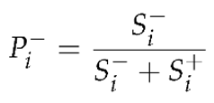
Final step is to calculate the relative performance score for each scenario within the dataset.

Based on the relative performance scores, the range of these scores have been equally distributed into 4 different classes with specified ranges resulting in the classified dataset with the corresponding classes assigned as shown in
Table 5. Using this algorithm, out of the 1000 scenarios, there were 76 scenarios identified as Class1, 368 scenarios identified as Class2, 453 scenarios identified as Class3 and 103 scenarios identified as Class4.
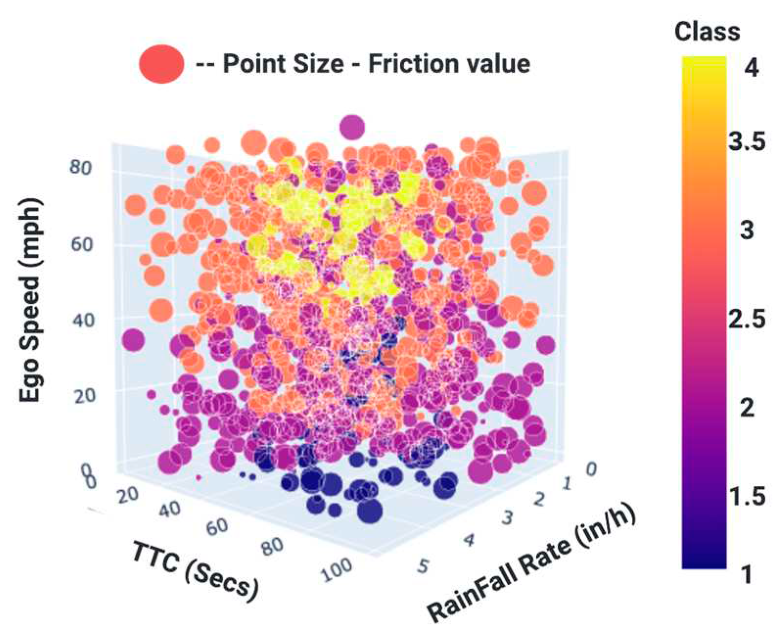
Figure 15 represents a 5-dimensional scatter plot with all 4 criteria plotted against the classes that have been determined using the TOPSIS algorithm. X-axis represents the RainFall Rates in inches/hour, Y-axis represents the TTC values, Z-axis represents the Ego vehicle speed values, size of the scatter plot data points represent the Friction values, color of the scatter plot data points represents the classes and the corresponding heat map has been provided. This type of plot helps visualize the mapping of the multiple criteria and their values being considered in the generated data to their corresponding classes.
Hence, this example provides one way of classifying the scenarios using known MDCM method like TOPSIS. This work can be extended to use more Machine Learning (ML) and Deep Learning techniques to enhance the performance of the classification using decision trees and random forest algorithms.
6. Conclusion
This paper outlines a systematic approach to defining the Operational Design Domain (ODD), system capabilities, and scenarios, providing guidance for developing Level 2, 3, and 4 autonomy systems. It traces the evolution of safety limits, identifies scenario classification parameters for the Decision-Making (DM) Engine, and describes the primary functions of each autonomy stack layer concerning safety limits application. The classification of safety limits into four categories is presented, offering a similar reference to ISO26262 severity or risk levels. The analysis includes real vehicle platforms and tests, informing the classification of actuation values into limits classes using scenario case studies from existing driving logs. These limits are stored in a cloud database, reducing on-board computing resources and promoting fleet-wide utilization. The paper concludes with an example DM algorithm for detecting "Driving in Rain" scenarios, demonstrating the applicability of the proposed classification framework to various scenarios and use cases in the industry’s journey toward Level 5 Autonomy.
7. Future Work
MCDM algorithms could benefit from integration with Machine Learning (ML) and Deep Neural Networks (DNNs) to address increasing complexity with a growing number of criteria. For handling overlapping classes, which are beyond this paper’s scope, fuzzy logic or DNNs might offer more effective solutions. Ongoing work explores the use of ML and DNNs, with results to be included in future publications.
To enhance the accessibility and accuracy of the cloud database, a connected vehicle concept using Vehicle-to-Infrastructure (V2I) communication can involve multiple Original Equipment Manufacturers (OEMs) and entities contributing and subscribing. Further developments should incorporate more ML and Deep Learning algorithms for precise scenario prediction and classification, aiming to refine the correlation between classes over time. Another potential extension involves creating driver models with varying degrees of passiveness or aggressiveness, aligning with human behavior studies, and mapping classes to different driving modes (normal, eco, sport) [
40,
41]. These additions can introduce more granularity and versatility to the system adding the human machine interaction parameter set in determining the limits.
References
- Johnson, Matthew C. Development of a robotic vehicle control system. PhD diss. 2013.
- Ma, C.; Xue, J.; Liu, Y.; Yang, J.; Li, Y.; Zheng, N. Data-Driven State-Increment Statistical Model and Its Application in Autonomous Driving. IEEE Trans. Intell. Transp. Syst. 2018, 19, 3872–3882. [Google Scholar] [CrossRef]
- Ku, I.; Lu, Y.; Gerla, M.; Gomes, R.L.; Ongaro, F.; Cerqueira, E. Towards software-defined VANET: Architecture and services. In Proceedings of the 2014 13th Annual Mediterranean Ad Hoc Networking Workshop (MED-HOC-NET), Piran, Slovenia; 2014; pp. 103–110. [Google Scholar] [CrossRef]
- Garikapati, D.; Liu, Y. Dynamic Control Limits Application Strategy For Safety-Critical Autonomy Features. In Proceedings of the 2022 IEEE 25th International Conference on Intelligent Transportation Systems (ITSC), Macau, China; 2022; pp. 695–702. [Google Scholar] [CrossRef]
- Taxonomy and Definitions for Terms Related to Driving Automation Systems for On-Road Motor Vehicles J3016_202104. J3016_202104: Taxonomy and Definitions for Terms Related to Driving Automation Systems for On-Road Motor Vehicles – SAE International.
- Hajiloo, R.; Abroshan, M.; Khajepour, A.; Kasaiezadeh, A.; Chen, S.K. Integrated steering and differential braking for emergency collision avoidance in autonomous vehicles. IEEE Transactions on Intelligent Transportation Systems 2020, 22, 3167–3178. [Google Scholar] [CrossRef]
- Funke, J.; Brown, M.; Erlien, S.M.; Gerdes, J.C. Collision Avoidance and Stabilization for Autonomous Vehicles in Emergency Scenarios. IEEE Transactions on Control Systems Technology 2016, 25, 1204–1216. [Google Scholar] [CrossRef]
- Tang, L.; Kacprzynski, G.J.; Goebel, K.; Saxena, A.; Saha, B.; Vachtsevanos, G. Prognostics-enhanced Automated Contingency Management for advanced automated systems. 2008 International Conference on Prognostics and Health Management, Denver, CO, USA, 2008, pp. 1-9. [CrossRef]
- PAS 1883:2020 Operational Design Domain (ODD) taxonomy for an automated driving system (ADS) – Specifi cation. Published by BSI Standards Limited 2020. ISBN 978 0 539 06735 4 ICS 03.220.20; 35.240.60.
- Schwarting, W.; Alonso-Mora, J.; Rus, D. Planning and Decision-Making for Autonomous Vehicles. Annu. Rev. Control. Robot. Auton. Syst. 2018, 1, 187–210. [Google Scholar] [CrossRef]
- ISO/CD PAS 8800 - Road Vehicles — Safety and artificial intelligence.
- AVSC00002202004: AVSC Best Practice for Describing an Operational Design Domain: Conceptual Framework and Lexicon – SAE International.
- ISO 34503:2023, Road Vehicles Test scenarios for automated driving systems Specification for operational design domain.
- U.S. Department of Transportation, National Highway Traffic Safety Administration, 2018. A Framework for Automated Driving System Testable Cases and Scenarios. DOT HS 812 623.
- Dawson, J.; Garikapati, D. Extending ISO26262 to an Operationally Complex System. In Proceedings of the 2021 IEEE International Systems Conference (SysCon), Vancouver, BC, Canada; 2021; pp. 1–7. [Google Scholar] [CrossRef]
- Sedghi, L.; Ijaz, Z.; Rahim, N.A.; Witheephanich, K.; Pesch, D. Machine Learning in Event-Triggered Control: Recent Advances and Open Issues. IEEE Access 2022, 10, 74671–74690. [Google Scholar] [CrossRef]
- Zhou, J.; Beyerer, J. Corner Cases in Data-Driven Automated Driving: Definitions, Properties and Solutions. In Proceedings of the 2023 IEEE Intelligent Vehicles Symposium (IV), Anchorage, AK, USA; 2023; pp. 1–8. [Google Scholar] [CrossRef]
- Cai, J.; Deng, W.; Guang, H.; Wang, Y.; Li, J.; Ding, J. A Survey on Data-Driven Scenario Generation for Automated Vehicle Testing. Machines 2022, 10, 1101. [Google Scholar] [CrossRef]
- Hendrik.A.Reese, Driving ! = Driving: Why operational design domain and scenario definition is the essence for safe autonomous driving systems.
- Koopman, P.; Widen, W. Safety Ethics for Design and Test of Automated Driving Features. IEEE Des. Test 2023, 41, 17–24. [Google Scholar] [CrossRef]
- Elliot Weiss, J. Christian Gerdes. Follow My Lead: Designing an ADAS that Shares Decision Making and Control with the Driver. In Proceedings of the 2023 IEEE Conference on Systems, Man, and Cybernetics (SMC), October, 2023. [Google Scholar]
- Kegelman, J.C.; Harbott, L.K.; Gerdes, J.C. Insights into vehicle trajectories at the handling limits: analysing open data from race car drivers. Vehicle System Dynamics 2017, 55, 191–207. [Google Scholar] [CrossRef]
- Goh, J. , Gerdes, J. C., Bobier-Tiu, C., Pavone, M., Rock, S. M., & Stanford University. (2019). Automated vehicle control beyond the stability limits.
- FUNKE, J. , GERDES, J. C., MITIGUY, P., & PAVONE, M. (2015). Collision avoidance up to the handling limits for autonomous vehicles.
- Song, Q.; Tan, K.; Runeson, P.; Persson, S. Critical scenario identification for realistic testing of autonomous driving systems. Softw. Qual. J. 2022, 31, 441–469. [Google Scholar] [CrossRef]
- Yuen, K.F.; Chua, G.; Wang, X.; Ma, F.; Li, K.X. Understanding Public Acceptance of Autonomous Vehicles Using the Theory of Planned Behaviour. Int. J. Environ. Res. Public Health 2020, 17, 4419. [Google Scholar] [CrossRef] [PubMed] [PubMed Central]
- Sitinjak, C.; Tahir, Z.; Toriman, M.E.; Lyndon, N.; Simic, V.; Musselwhite, C.; Simanullang, W.F.; Hamzah, F.M. Assessing Public Acceptance of Autonomous Vehicles for Smart and Sustainable Public Transportation in Urban Areas: A Case Study of Jakarta, Indonesia. Sustainability 2023, 15, 7445. [Google Scholar] [CrossRef]
- Martin, H.; Winkler, B.; Grubmüller, S.; Watzenig, D. Identification of performance limitations of sensing technologies for automated driving. In Proceedings of the 2019 IEEE International Conference on Connected Vehicles and Expo (ICCVE), Graz, Austria, 2019; pp. 1–6. [Google Scholar] [CrossRef]
- Yeong, D.J.; Velasco-Hernandez, G.; Barry, J.; Walsh, J. Sensor and Sensor Fusion Technology in Autonomous Vehicles: A Review. Sensors 2021, 21, 2140. [Google Scholar] [CrossRef] [PubMed]
- Aufrère, R.; Gowdy, J.; Mertz, C.; Thorpe, C.; Wang, C.-C.; Yata, T. Perception for collision avoidance and autonomous driving. Mechatronics 2003, 13, 1149–1161, ISSN 0957. [Google Scholar] [CrossRef]
- Riedmaier, S.; Ponn, T.; Ludwig, D.; Schick, B.; Diermeyer, F. Survey on Scenario-Based Safety Assessment of Automated Vehicles. IEEE Access 2020, 8, 87456–87477. [Google Scholar] [CrossRef]
- Rodionova, A.; Alvarez, I.; Elli, M.S.; Oboril, F.; Quast, J.; Mangharam, R. How safe is safe enough? Automatic Safety Constraints Boundary Estimation for Decision-Making in Automated Vehicles. In Proceedings of the 2020 IEEE Intelligent Vehicles Symposium (IV), Las Vegas, NV, USA, 2020, pp. 1457-1464. [CrossRef]
- Li, S. , Yang, J., Chen, W., Chen, X. (2014). Disturbance Observer-Based Control: Methods and Applications. United Kingdom: Taylor & Francis.
- Kouro, S.; Cortes, P.; Vargas, R.; Ammann, U.; Rodriguez, J. Model Predictive Control—A Simple and Powerful Method to Control Power Converters. IEEE Trans. Ind. Electron. 2008, 56, 1826–1838. [Google Scholar] [CrossRef]
- Koibuchi, K.; Yamamoto, M.; Fukada, Y.; Inagaki, S. Vehicle Stability Control in Limit Cornering by Active Brake. SAE Technical Paper 96 0487, 1996. [Google Scholar] [CrossRef]
- ISO 26262-1:2018 Road vehicles Functional safety, International Standard under systematic review [90.20], vol.2(33),ISO/TC 22/SC 32, ICS : 01.040.43 43.040.10.
- Laurense, V.A.; Goh, J.Y.; Gerdes, J.C. Path-tracking for autonomous vehicles at the limit of friction. In Proceedings of the 2017 American Control Conference (ACC), Seattle, WA, USA; 2017; pp. 5586–5591. [Google Scholar] [CrossRef]
- Hoback, A.S. Relationships between aggressive driving behaviors, demographics and pareidolia. Transportation Research Interdisciplinary Perspectives 2019, 2, 100037, ISSN 2590–1982. [Google Scholar] [CrossRef]
- Wang, Z.; Liao, X.; Wang, C.; Oswald, D.; Wu, G.; Boriboonsomsin, K.; Barth, M.J.; Han, K.; Kim, B.; Tiwari, P. Driver Behavior Modeling Using Game Engine and Real Vehicle: A Learning-Based Approach. IEEE Trans. Intell. Veh. 2020, 5, 738–749. [Google Scholar] [CrossRef]
- Melman, T.; de Winter, J.; Mouton, X.; Tapus, A.; Abbink, D. How do driving modes affect the vehicle’s dynamic behaviour? Comparing Renault’s Multi-Sense sport and comfort modes during on-road naturalistic driving. Veh. Syst. Dyn. 2019, 59, 485–503. [Google Scholar] [CrossRef]
- Kenny Longdon. Driving Modes Explained: What are They? Evans Halshaw, Nov 2022.
- Qin; Joe, S.; Badgwell, T.A. An overview of industrial model predictive control technology. AIche symposium series. Vol. 93. No. 316. New York, NY: American Institute of Chemical Engineers, 1971-c2002., 1997.
- Liang, Z.; Zhao, J.; Liu, B.; Wang, Y.; Ding, Z. Velocity-Based Path Following Control for Autonomous Vehicles to Avoid Exceeding Road Friction Limits Using Sliding Mode Method. IEEE Trans. Intell. Transp. Syst. 2020, 23, 1947–1958. [Google Scholar] [CrossRef]
- Triantaphyllou, E. (2000). Multi-Criteria Decision Making Methods. In: Multi-criteria Decision Making Methods: A Comparative Study. Applied Optimization, vol 44. Springer, Boston, MA. [CrossRef]
- Olson, D. Comparison of weights in TOPSIS models. Math. Comput. Model. 2004, 40, 721–727. [Google Scholar] [CrossRef]
- Naser, Felix et al. A Parallel Autonomy Research Platform. In Proceedings of the 2017 IEEE Intelligent Vehicles Symposium, IEEE, Redondo Beach, CA, USA, 11-14 June, 2017.
|
Disclaimer/Publisher’s Note: The statements, opinions and data contained in all publications are solely those of the individual author(s) and contributor(s) and not of MDPI and/or the editor(s). MDPI and/or the editor(s) disclaim responsibility for any injury to people or property resulting from any ideas, methods, instructions or products referred to in the content. |
© 2024 by the authors. Licensee MDPI, Basel, Switzerland. This article is an open access article distributed under the terms and conditions of the Creative Commons Attribution (CC BY) license (http://creativecommons.org/licenses/by/4.0/).

 and
and  non-ideal values
for each criteria from the previously normalized and weighted values. These values are then used to calculate the Euclidean distances to each criteria values in the dataset.