1. Introduction
In an aging world, accurate modelling of human mortality becomes crucial due to demographic transitions, catastrophic events, healthcare advancements, and societal shifts. Mortality models examine the factors influencing life expectancy, enabling pension plans, insurers, and actuaries to make informed decisions regarding healthcare planning, pension systems, and societal well-being. Since the early 1990s, researchers have developed numerous stochastic models to capture and quantify the patterns of human mortality over time. These models include the Lee-Carter model, its extensions and alternatives (Lee and Carter [
14], Brouhns et al. [
2], Renshaw and Haberman [
22]), the P-splines model (Currie et al. [
10]), and the Cairns et al. model [
4] [
5].
However, recent decades have witnessed significant changes in mortality rates in many countries. Generally, there has been an improving trend, but for some, the last 10 to 20 years have seen either a slowdown or even a reversal of some of these improvements, further disrupted by the COVID pandemic [
3]. Catastrophic events such as COVID-19 are referred to as mortality risks, and they may cause sudden increases in mortality rates over certain periods of time. While these events are infrequent, their occurrences could lead to numerous death claims and mortality jumps on the mortality curve.
Particularly, COVID-19 has highlighted the crucial consequences of these catastrophic events and emphasised the importance of preparing for future outbreaks. Hence, it is essential to incorporate mortality jumps in the modelling process. Although many mortality models without jump effects exist, only a few models have been developed that consider mortality jump effects. These include Chen and Cox [
6], Cox et al. [
8], Deng et al. [
11], and Özen and Şahin [
18], which differ in terms of the duration of the jumps - transitory or permanent, frequency of the jumps, and size of the jumps.
To provide a comprehensive overview, Regis and Jevtic [
20] also present a review of single and multi-population mortality models with and without jumps. Specifically, they focus on multi-population mortality models with jumps since these models are needed to describe the heterogeneous impact of mortality shocks across cohorts of individuals. An example of a two-population model with jump effects can be found in Özen and Şahin [
19].
In this study, we aim to compare and discuss the performance of mortality models, both with and without jump effects, analysing their ability to capture the mortality deterioration caused by COVID-19. The mortality models without jump effects include the Lee-Carter model, Renshaw and Haberman model, and Cairns-Blake-Dowd model. In contrast, the Lee-Carter model with permanent jump effects, transitory jump effects, exponential transitory jumps, and renewal process effects are employed as the mortality models with jump effects. We utilise mortality data from various countries obtained from the Human Mortality Database (HMD) [
13]. Given that COVID-19 is a potential cause for a jump in the mortality curve, our primary objective is to identify the mortality models that can accurately forecast COVID deaths from 2020 onwards. To achieve this, we initially fit the data to the models and simulate the mortality rates to make forecasts for the pandemic years.
Furthermore, we present the pricing of catastrophe bonds using the mortality model with jump effects. We derive the market prices of mortality jump risks by applying the Swiss-Re bond to all mortality models with jump effects.
The remainder of this paper is structured as follows:
Section 2 describes the mortality models utilised in this study.
Section 3 presents the results and compares the models in terms of model parameters, model fits, in-sample, and out-of-sample forecasts.
Section 4 provides an example of pricing mortality-linked security. Finally,
Section 5 concludes the paper.
2. Mortality Models
This section introduces the mortality models considered in this study. To provide a comprehensive analysis of mortality jump models and their performance in forecasting COVID-19 deaths, we compare them with the Lee-Carter (LC) model [
14] with random walk which serves as the benchmark model. Additionally, we include the Renshaw and Haberman (RH) [
21] model as a representative of age-period-cohort (APC) models and the Cairns-Blake-Dowd (CBD) [
4] model as the two-factor mortality model. While we briefly introduce models without jump effects for completeness, the primary focus of the study is to discuss mortality models with jump effects.
2.1. The Lee-Carter Model
In the Lee-Carter model [
14],
denotes the central death rate of age group
x in year
t. The model is expressed as:
Here,
is the average of
over time
t, and
represents the general shape of the mortality rates. The mortality time index
, capturing the variation of log mortality rates over time, is modulated by an age response
that represents how slowly or rapidly mortality at each age varies when the mortality index changes.
is the error term, capturing age-specific effects not reflected in the model. Model parameters can be estimated using a two-stage singular value decomposition (SVD) or the maximum likelihood estimation (MLE) method. As indicated by [
2], estimation results from both methods are almost the same. The SVD method requires the following constraints:
The estimation is a two-stage process. First, the SVD method is applied to the matrix of
to obtain estimates of
and
. Second, the time-varying terms are re-estimated by iteration, given the values of
and
. This ensures the actual sum of deaths at time
t equals the implied sum of deaths at time
t:
where
is the actual sum of deaths at time
t, and
is the population in age group
x at time
t.
In this paper, following [
2] and using the StMoMo R Package [
23], we employ the MLE method to estimate the parameters. We fit the Lee-Carter model assuming a Poisson distribution of the number of deaths, using the log link function to target the force of mortality
. Hence, the predictor
is given by:
We adopted the notation from [
23]. In the original Lee-Carter model, the
parameters are modelled using a random walk with drift, as in Equation (
2):
where
has a standard normal distribution.
The Lee-Carter model with a random walk is considered as a benchmark model in this paper.
2.2. Renshaw and Haberman Model
As a second model, we use the age-period-cohort model proposed by Renshaw and Haberman [
21], which is an extension of the Lee-Carter model.
Here, represents the cohort effect. Mortality projections for this model are obtained by forecasting the time series of the estimated and as univariate ARIMA processes under the assumption of independence between the period and cohort effects.
2.3. Cairns-Blake-Dowd Model
Cairns et al. [
4] proposed a mortality model with two age-period terms with pre-specified age-modulating parameters
and
, no cohort effect, and no static age function. The CBD model is given as follows:
where
is the average age in the data. The period effects
and
are modelled by using a bivariate random walk with drift to obtain mortality forecasts [
23].
2.4. Jump Effect Models as Extensions to the Lee-Carter Model
While the Lee-Carter model is inherently designed for long-term mortality analysis, its time-varying mortality index must incorporate short-term effects to enhance the efficacy of mortality modelling. This necessity has led to the introduction of jump effect models.
In this section, we will present one permanent jump model and two transitory jump models. These models are regarded as extensions of the Lee-Carter model as they specifically address the time-varying parameter and incorporate explicit jump effects.
2.4.1. with Permanent Jump Effect
Cox, Lin, and Wang [
8] proposed a mortality model with permanent jump effects, combining geometric Brownian motion and a compound Poisson process. However, we consider the model in a discrete-time setting, following Chen and Cox [
6], for the consistency of model comparisons.
Therefore, let
denote the number of jumps occurring in year
t. For simplicity, it is assumed that there is at most one jump event in each year, with the probability of a jump being
p. That is,
The jump severity variable, Y, is identically and independently distributed normal variables with mean m and standard deviation s. Moreover, Y and N are independent.
As in [
6], the evolution of the mortality index
with permanent jump effects can be written as
where
and
are constants, and
is a standard normal random variable that is independent of
Y and
N.
2.4.2. with Transitory Jump Effect
In the permanent jump model, if a jump event occurs in year , the size of the jump is incorporated into the mortality factor , and this jump effect persists indefinitely. However, many of these jumps are attributed to short-term catastrophic events, resulting in a transient impact on the mortality curve. Therefore, mortality models with transitory jump effects are deemed more suitable for modelling extreme mortality risks.
We consider the transitory jump effects as proposed by Chen and Cox [
6]. In their model, the mortality factor is modelled as follows:
where
denotes the jump-free mortality factor, and
is the actual mortality factor including jumps.
Equation (
5) indicates that extreme mortality events only have an impact on
, not on
. Therefore, if a mortality jump occurs in a given year, it will revert to the normal mortality level shortly thereafter.
2.4.3. with Exponential Transitory Jumps and Renewal Process Effect
The model with exponential jumps and a renewal process is proposed by Özen and Şahin [
18]. The originality of the model lies in the usage of the renewal process instead of the Poisson process. In the Poisson process, waiting times between mortality jumps are constant, meaning that the occurrence of previous catastrophic events has no impact on the likelihood of the next event. To incorporate the history of events, one approach is to consider the renewal process, featuring a time-varying hazard function reflecting the waiting times between catastrophic events. An increasing hazard function indicates longer waiting times between events than a decreasing hazard function. In these models, waiting times between catastrophic events are no longer constant; however, the occurrence of at least one event (versus none) up to time
t influences the probability of another event’s arrival in
by the time-varying hazard function. Hence, by employing the renewal process, we aim to integrate the history of catastrophic events into the mortality modelling process.
In the proposed model, the mortality factor is modelled as:
where
is standard Brownian motion,
is a renewal process with parameters
and
. The expected value of the process would give the expected frequency of the jumps. Here,
denotes a sequence of independent and identically distributed exponential random variables representing the size of the jumps with parameter
. The terms
and
denote the expected value of the jump size and the jump frequency, respectively.
In the renewal process, to calculate jump probabilities, we need to specify the distribution of the inter-arrival times between mortality jumps. Therefore, we must first detect the mortality jumps on the mortality curve. This is achieved by employing the method proposed by Chen and Liu [
7] to identify outliers in the mortality index. The outlier detection approach classifies the outliers into four categories based on their impacts on the time series. In this study, we focus on the additive outliers since they have one short and immediate effect on the time series [
6]. After performing the outlier detection process and obtaining the additive outliers on the mortality curve, as in Li and Chan ([
16]), we consider the events as outliers that are greater than the critical value of
. Thereafter, we need to specify the inter-arrival times between these events. The years of detected outliers and their test statistics are shown in
Table 1. Subsequently, we determine the distributions of the inter-arrival times of jumps to make predictions for future expected frequencies of outliers (for model details, refer to [
18]).
However, this process requires a decent sample size for distribution fitting. The detected outliers are given in
Table 1, showing 7 outliers for Spain, Sweden, and Switzerland; 5 for Denmark, 3 for the UK, and 2 for Japan. This indicates that the size of the data to fit a distribution for inter-arrival times is 6 for three countries in the best case. It is still too few to fit a distribution properly.
The literature on the topic suggests lognormal, Weibull, and gamma distributions [
17]. Due to the small number of jumps and hence inter-arrival times, we consider the distributions proposed by the existing literature and compare the log-likelihoods and BICs of the overall model for each distribution. Then, we choose the distribution for the inter-arrival times that provides the best fit for each country. Therefore, the analysis reveals that the distributions of inter-arrival times are lognormal for Denmark and Switzerland and Weibull for Japan, Spain, Sweden, and the UK.
Based on the specified distribution, convolution methods are used to obtain the jump frequencies in the renewal process. Let
be the probability of
n jumps occurring in the given time. Moreover,
and
are the distribution and density functions of the inter-arrival times between jumps. Then, the jump probabilities are obtained by
and
(for more details, see [
18]).
Table 1 presents the years of the detected outliers for Denmark, Japan, Spain, Sweden, Switzerland, and the UK after fitting time series models to the obtained
values using the Lee-Carter model. It is crucial to note that the detected years are subject to change due to the fitted time series model. We selected the best-fitting models, which are outlined in the table. The provided years for outliers, hence, mortality jump years, are determined based on the residuals from the given time series models. Notably, for Japan, those two jumps coincide with the Fukui earthquake (1948) and Isahaya flood (1957); for Spain, we observe 7 jumps - 1918-1919 represents the Spanish Flu, and 1942 represents the Civil War. Likewise, for Sweden and Switzerland, we observe 7 jumps - 1918-1919 represents the Spanish flu. In the case of the UK, three jumps are observed, with 1944 representing World War II.
Table 1 also presents the mean absolute percentage errors (MAPE) for each country. As demonstrated in the next section,
over time for Japan during the fitted period is notably smooth compared to the other countries, suggesting minimal indications of jumps in the mortality index.
In Appendix A1, we utilised all available up-to-date data for six countries to observe and compare the number of jumps and jump years in pre- and post-COVID periods. For Spain, Sweden, Switzerland, and the UK, the COVID pandemic caused statistically significant jumps based on the outlier analysis discussed above. The inclusion of the COVID years either increased the number of observed jumps or changed the observed jump years while keeping the number of jumps the same for the time index parameter.
3. Results and Discussion
This section presents results from different models for each country to compare and discuss their fits to the historical data and the performance of the models for forecasting COVID-19 deaths from 2020 onwards.
3.1. Model Comparisons
3.1.1. Fitted parameters
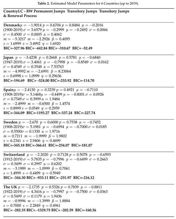
Firstly, we present the parameters obtained from the fitted LC model for each country and proceed to compare these estimates with those derived from three distinct jump models: with a permanent jump, with a transitory jump, and with a renewal process.
Figure 1 visually represents the comparison, highlighting that the
parameters obtained from the transitory jump models exhibit a closer alignment with the original LC parameters across all examined countries.
The utilisation of jump models is particularly insightful, as they contribute to the production of smoother trajectories by explicitly incorporating jumps in the mortality time index. A smoother trajectory that closely mirrors the LC parameter is indicative of a superior fit.
As demonstrated in
Figure 1, the permanent jump model consistently and notably underestimates the time-dependent parameters in Spain, while frequently overestimating
for Denmark, Sweden, Switzerland, and the UK in comparison to the LC parameter. In contrast, both transitory jump models yield more accurate fits. The renewal process utilising the exponential jump model is particularly noteworthy, as it generates trajectories that closely correspond to the LC parameter across all six countries.
It is crucial to acknowledge that, in the case of Japan, the limited number of jumps during the considered period complicates the applicability of any of the jump models. Consequently, none of the models appear to be ideal for this specific scenario. This observation highlights the intricate challenges inherent in mortality jump modelling, especially in situations where jump occurrences are sparse.
3.1.2. Bayes Information Criterion
The Bayes Information Criterion (BIC) serves as a means to compare models and discern which one better fits the data. A key aspect of BIC is its ability to compare models that are not necessarily nested.
The BIC for mortality models is defined as:
Here,
denotes the parameter vector, and
stands for its maximum likelihood estimate. In this context,
represents the maximum likelihood,
N is the number of observations, and
is the number of parameters estimated from the mortality models [
5].
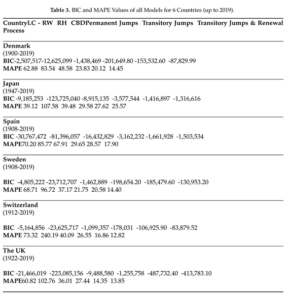
To determine which jump effect better fits the mortality data, we initiate the comparison by examining the mortality time indices (for estimated s), parameter estimations, and BIC values obtained for those s in Table 2. Subsequently, we extend our comparison to encompass all jump-free and jump models, evaluating their overall BIC values (not limited to s alone) as presented in Table 3. It is noteworthy that a higher BIC value indicates a better fit.
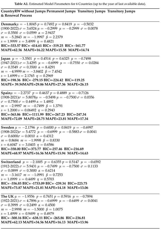
Table 2 presents a comparative analysis between the Lee-Carter with random walk (LC - RW) model and three jump models, all fitted to the parameters derived from the benchmark LC model and its derivatives. Among these models, the two transitory jump models exhibit superior fits, as evidenced by their lower BIC values, in contrast to both the LC-RW (except Japan for one of the models) and permanent jump model. It is essential to note that while the differences in BIC values may seem substantial, a more dependable basis for comparing the performance of the models is provided by the mean absolute percentage errors (MAPE), which is discussed in the following subsection. In Appendix A2, we utilised all available up-to-date data for six countries to observe changes in model parameters and in-sample fits for pre- and post-COVID periods. The results indicate that although including COVID data changed the parameters, the performance of the models did not change significantly.
On the other hand, Table 3 offers a more detailed comparison among three jump-free models—namely, LC-RW, RH, and CBD—and three jump models derived from the LC model. This comparison is facilitated by presenting the overall model BICs and MAPEs. Given the diverse structures of the models, the BIC values appear quite distinct. However, it is evident that, in general, and particularly with transitory jump models, the jump models consistently outperform the benchmark jump-free models.
3.1.3. Mean Absolute Percentage Error (MAPE)
The mean absolute percentage error (MAPE) stands out as a widely used metric for assessing prediction accuracy in mortality modelling. Its formulation is given by:
In this equation, represents the number of observations in each population, calculated as the product of the number of ages and the number of years. Here, denotes the estimated number of deaths, while represents the observed number of deaths for a specific time (t), age (x), and population (i).
We employ MAPE to assess the in-sample prediction performance of the models. Initially, we consider all ages in Table 3 as model MAPEs. Subsequently, we present graphs for specific ages (20, 40, 60, and 80) to observe age-specific variations, focusing exclusively on jump models for different countries in
Figure A1,
Figure A2,
Figure A3,
Figure A4,
Figure A5,
Figure A6 in Appendix. These graphs share a common y-scale, facilitating the comparison of different models and their effectiveness in capturing mortality deterioration across various countries.
Contrary to the BIC values, the overall MAPE values in Table 3 present a much closer scale when comparing jump-free and jump models. However, the LC-RH model stands out by producing relatively distinct and higher MAPEs compared to the others. Consistently lower MAPEs obtained from the jump models indicate better fits for the listed countries, with transitory jump models—particularly the renewal process model—exhibiting superior fits.
Furthermore, the MAPE results illustrated in
Figure A1,
Figure A2,
Figure A3,
Figure A4,
Figure A5,
Figure A6 in Appendix indicate that better fits, characterised by lower MAPE values and reduced volatilities, are observed as ages increase for almost all countries and all three models. Notable differences emerge between the models, with the two transitory jump models consistently demonstrating superior fits and yielding the lowest MAPE values across all countries and ages, except for Japan.
The model incorporating an exponential jump with the renewal process consistently provides the lowest MAPE for all countries and ages, with the same exception—Japan, despite the volatilities observed in the graphs. Additionally, for Japan, the LC-RW model exhibits a slightly better fit as age advances, a detail not clearly depicted in the graphs. This observation aligns with the parameter graphs in the preceding section for Japan, where the time series graph appears notably smoother, suggesting fewer significant jumps compared to other countries discussed in this paper. Essentially, this implies that when there are no jumps or only a few jumps, regardless of their frequency, jump-free models tend to outperform models with jumps.
3.1.4. Forecasts
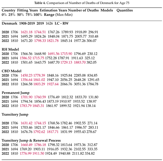
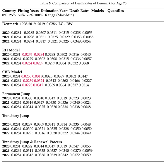
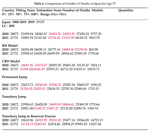
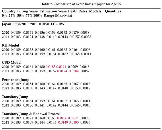
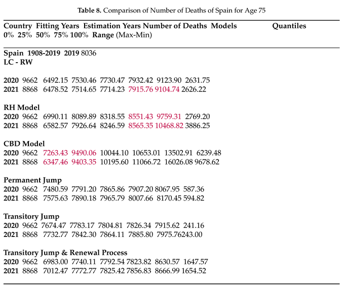
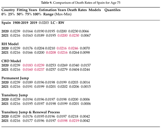
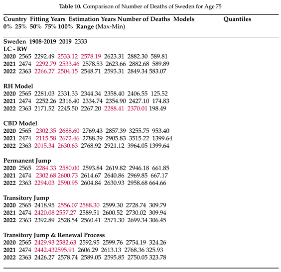
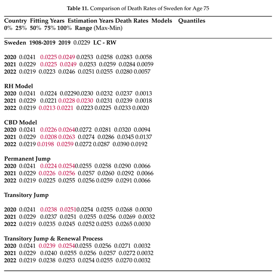
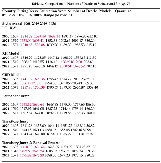
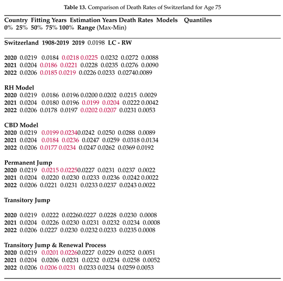
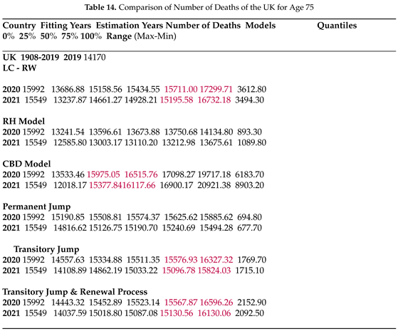
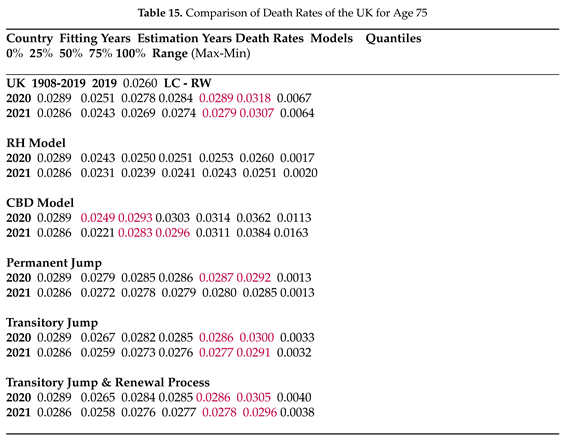
Table 4 to Table 15 present forecasts for the COVID and post-COVID years, including quantiles and ranges derived from 100,000 simulations, along with the observed number of deaths and death rates (obtained by dividing the number of deaths by 2019 exposures) for age 75, serving as an example for six countries. The models, encompassing both jump-free and explicit jump models, were fitted up to 2019, the last pre-COVID year, and are compared in forecasting COVID deaths for the COVID and post-COVID years based on data availability from the HMD website.
In Table 4, only the CBD model forecasts COVID deaths for all three years from 2020 to 2023 for Denmark, with relatively high uncertainty compared to the other models. The LC-RW model captures the number of deaths for 2020 in the first quantile, along with the CBD and all three jump models, while the RH provides true forecasts for deaths at age 75 in the third quantile. Comparing to the number of deaths in the last pre-COVID year (2019) in Denmark, the jump models forecast the number of deaths for 2020 and 2022 in the first quantile with relatively small uncertainty given as the range in the final column. However, in Table 5, when we obtained the death rates by dividing the simulated number of deaths by the 2019 exposure, neither the LC-RW nor the jump models capture true rates. Jump models forecast higher death rates based on the 2019 exposures.
For Japan, in Table 6 all six models provide forecasts with varying degrees of uncertainty. RH, permanent jump, and transitory jump models offer smaller forecast intervals compared to the other two jump-free benchmark models. The transitory jump model with the renewal process presents a less accurate fit, consistent with its structure, which requires the distribution of inter-arrival times, a challenge when only two observations are available. It is important to note that the number of deaths in 2019 for age 75 is higher than the COVID and post-COVID years. Table 7 shows the death rates based on 2019 exposures, and only the CBD model and the transitory jump model with the renewal process seem to provide true forecasts at the expense of including high uncertainty.
In Table 8, only the jump-free models capture the high jump in the first COVID year (2020) in Spain with a huge range of forecasts. Jump models, although providing smaller forecast intervals, perform less accurately. On the other hand, Table 9indicates that the transitory jump model with renewal process manages to forecast the death rate for 2021 with much smaller uncertainty.
For Sweden in Table 16, except for the RH model, which only forecasts 2022 correctly, all other models forecast COVID deaths within the provided ranges for at least first two years (2020 and 2021). Jump models, particularly transitory jump models, offer more accurate forecasts with smaller ranges, although in Table 11, it causes the exclusion of the correct range for 2021 and 2022 when using the 2019 exposure.
Table 12 shows that the LC-RW and CBD models forecast the number of deaths for all three years from 2020 to 2022 with relatively large uncertainty compared to the transitory jump model with the renewal process for Switzerland. The permanent jump model provides the smallest ranges while forecasting the first year within the range. The performance of the models for forecasts for the death rates in Table 13 does not differ significantly from the number of deaths.
In the UK (Table 14), there is a notable jump in the number of deaths due to COVID compared to 2019, and except for the RH and permanent jump models, the other four models for the following two years manage to include the number of deaths in their forecast ranges, although the CBD model produces extremely large forecast intervals. In Table 15, two transitory jump models provide the correct death rates with more accuracy compared to the LC-RW and the CBD models, while the permanent jump model forecasts 2020 death rates within the range different from the number of death results.
When we consider younger ages, such as 60, none of the jump models accurately predicted the high number of deaths for Spain or the UK.
All six models perform differently for different countries. The CBD model successfully forecasts COVID deaths for a higher number of countries and years under examination. However, it is worth noting that the model produces wider intervals for the quantiles, which may not necessarily provide informative insights, as demonstrated in the cases of Spain, Sweden, and the UK.
4. Pricing of Mortality-Linked Securities
This section delves into the impact of mortality models with jump effects on the market pricing of extreme mortality risk. Estimating the market price of risk is crucial as it sheds light on the investor’s reward for assuming extreme mortality risk.
The securitisation of human life has been a significant financial innovation for life insurance companies since late 1980s. Enhancing the value of a firm through securitisation involves minimizing agency costs, transaction costs, regulatory requirements, and taxation [
9]. In recent years, reinsurers have sought to mitigate exposure to extreme mortality risk by issuing catastrophic mortality bonds. These bonds typically have relatively short maturity times, often three or five years. Coupon payments are linked to a market interest rate such as the London Interbank Offered Rate (LIBOR), while the principal repayment is not guaranteed. The principal is reduced if the underlying index exceeds the attachment point and is exhausted if the index surpasses an exhaustion point.
To attract investors with varying objectives and risk preferences, a catastrophic mortality bond may be divided into several tranches, each having its attachment and exhaustion points, coupon rates, credit rating, and/or time to maturity [
15].
However, similar to mortality securities, the modeling of mortality securitisation is in the early stages of development, making the pricing of these instruments challenging. The absence of a complete market for mortality securities makes it impossible to determine a unique market price for risk.
In an incomplete market, there are primarily two approaches for security valuation. One way is to adopt the arbitrage-free pricing framework of interest-rate derivatives. The second method involves using a distortion operator to create an equivalent risk-adjusted distribution and obtain the fair value of the security under this risk-neutral measure [
6].
A common theme in the pricing and valuation of risks and contingent claims is the change of probability measure. In the no-arbitrage financial pricing theory, the price of a contingent claim is evaluated as the expected payoff under a risk-neutral probability measure different from its statistical counterpart [
12]. The risk-neutral probability measure can be inferred from market transaction data in a complete market. In an incomplete market, where there is insufficient market data to infer a risk-neutral distribution, we may rely on historical data to estimate the statistical distribution of potential outcomes and their respective likelihoods [
8]. Methods such as the Wang transform, a market-based equilibrium pricing method that unifies finance and insurance pricing theories [
24], can be employed for this purpose. Thus, we use the Wang transform to obtain the market prices of mortality risk based on different mortality models.
In this paper, we employ a hypothetical bond with specifications similar to the Swiss-Re mortality bond as an example to estimate the implied market prices of risk. While the payment structure and issue price remain the same, fundamental changes have been introduced, including the use of Swiss mortality, different attachments, and exhaustion points. Our primary goal is to ascertain the market prices of risk under various mortality jump models.
4.1. Design of the Swiss-Re Bond
Since mortality-linked instruments are traded in an incomplete market, we require an observed bond price to determine the market price of mortality risk, representing the price that pension funds or insurers are willing to pay to transfer mortality risk. Previous research articles (see [
1,
6]) have utilised the Swiss-Re mortality bond to ascertain the market price of mortality risk.
In December 2003, Swiss-Re insurance company introduced the first mortality risk contingent securitisation. If the bond is triggered by a catastrophic increase in death rates in a particular population, investors will lose principal and interest. The bond offers investors a higher yield as compensation for the mortality risk they undertake. The bond was issued through a special purpose vehicle called Vita Capital, enabling Swiss Re to remove extreme catastrophic risk from its balance sheet.
The bond had a maturity of 3 years, a principal of
million, and a coupon rate of 135 basis points plus the LIBOR rate. The mortality index,
, was a weighted average of mortality rates across five countries, males and females, and a range of ages. The principal was repayable in full only if the mortality index did not exceed 1.3 times the 2002 base level during any year of the bond’s life. If mortality did exceed this threshold, the payment was dependent on the realised values of the mortality index. The payment schedules were given by the following
functions:
where the function
specifies the amount of payment that is lost due to the mortality experience ([
11]).
As mentioned before, although the payment structure of the Swiss-Re bond remains the same, we have some fundamental differences. First, the mortality index of the bond is a weighted average across five countries. For simplicity, we assume the mortality index depends only on Switzerland’s mortality data. Moreover, based on our mortality data, we have different attachment and exhaustion points. For our case,
becomes
4.2. Change Measures via the Wang Transform
The Wang transform serves as a widely employed universal framework for pricing financial and insurance risks. For a given asset (or loss) variable X with a cumulative distribution function (CDF),
, the Wang transform produces a risk-adjusted CDF,
, given by the equation:
Here, represents the standard normal cumulative distribution, and denotes the market price of risk. After obtaining the risk-adjusted distribution , the expectation of X under , denoted by , can be calculated. By discounting this value back to time zero using the risk-free interest rate, we can determine the fair value of the asset (or loss) X.
The payoff of the mortality instrument considered in this article is based on three different jump models. The first model is the permanent jump model. For comparison purposes, the Wang transform is applied to the same variables
Z,
Y, and
N (or
p for the permanent jump model) for all mortality models. Let
,
, and
represent the market prices of risk associated with each of the variables
Z,
Y, and
p. Then the dynamics of the mortality factor under the risk-adjusted measure
Q becomes:
where
,
,
.
The second mortality model considered here is the transitory jump model, and after applying the Wang transform, the dynamics of the mortality factor under the risk-adjusted measure
Q becomes:
where
,
,
, and
([
6]).
The last mortality model is the transitory mortality jump with the renewal process model, and we use the Wang transform on the variables
Z,
Y, and
N. The risk-adjusted mortality factor becomes:
where
,
is distributed exponentially with the parameter
, and
.
Here, we apply the Wang transform to the expected jump frequency, which is different from other models. Since other mortality models with jumps assumed that mortality jumps could occur only once a year, they apply the Wang transform to the one-year jump probability. However, we assume that there could be more than one jump in a year; hence, we apply the Wang transform to the expected jump frequency.
We can derive the implied market price of risk
based on our hypothetical mortality bond. As mentioned before, our hypothetical bond is similar to the Swiss-Re bond. It has the same payment structure and issue price. However, our mortality index is a weighted average of Switzerland’s mortality rates. Age weights are obtained for all ages by dividing the exposures at each age by the total exposure. For the risk-free interest rate, Chen and Cox ([
6]) used the US Treasury yield rates on December 30, 2003. Here, we use Switzerland’s 10-year government bond yield rate on December 30, 2003, as the risk-free interest rate
1. Moreover, we calculate the coupon payments by assuming they are paid annually, as we do not have quarterly data for the Switzerland government bond yield.
The estimation procedure for calculating the market price of mortality risk for the hypothetical bond issued in 2003, based on the Wang transform and following the approach of Chen and Cox ([
6]), involves the following steps:
1. Simulate 10,000 times the future mortality time-series for 2004-2006 based on the known 2003 mortality time series, using the three mortality jump models.
2. Apply the Wang transform to transition from the physical measure
P to the risk-adjusted measure
Q. Calculate the values of
on each path under
Q using Equation
8,
9,
10, given initial values of the market prices of risk
, and
.
3. Calculate the mortality rates for different age groups by the formula under Q. Compute the weighted average mortality index for each year using , where denotes the weight assigned to the age group x based on the year 2003.
4. Calculate the expected value of principal payment in every period T by the formula . Calculate the coupon payment in every period based on the par spread plus 135 basis points obtained from the Swiss-Re bond.
5. Discount the coupon payments for each period and the principal repayment back to the beginning of the year 2004 using the risk-free rate. Equate the discounted expected payoff to the issue size of the Swiss-Re mortality bond (
$400 million) to obtain the market prices of risk using the quasi-Newton method, as in Chen and Cox ([
6]).
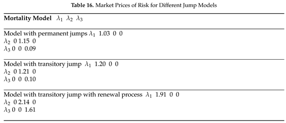
The estimated market prices of risk () for different jump models are presented in Table 16.
Under the permanent jump model, assuming that (indicating that the risk associated with the jump process is diversifiable), the market price of mortality risk is 1.03. If , the market price of risk associated with the jump size is 1.15. The market price of risk associated with the jump frequency is 0.09 if .
Shifting to the model with transitory jump effects, the market prices of risk increase in each case. This increase can be explained by differences in the model setups and the volatility of the mortality index. Higher volatility leads to higher risk and, consequently, lower market prices of risk.
Under the transitory mortality jumps with the renewal process model, the market prices of risk are the highest in each case. This implies that the model with transitory jumps with the renewal process offers a higher risk premium to investors, making the bond with this model more attractive to investors. Although a high market price of risk may suggest high transaction costs, it could also be interpreted as the hypothetical bond with transitory mortality jumps with the renewal process overcompensating investors for taking on its mortality risk ([
8]).
5. Conclusions
This paper aims to analyse the performance of mortality models with jump effects in forecasting COVID-19 deaths, focusing on six countries: Denmark, Japan, Spain, Sweden, Switzerland, and the UK. These models are also compared with benchmark mortality models such as LC, RH, and CBD models. The comparison involves mortality time indices, , in-sample prediction performances using BIC and MAPE, and out-of-sample forecasting performances based on the simulated forecasted number of deaths and death rates based on 2019 exposures for COVID and post-COVID years. While detailed results are discussed throughout the paper, more comprehensive conclusions can be drawn.
One significant observation is that the fit and forecast performance of mortality models, regardless of whether they include jump effects or not, heavily depends on the specific country, time, and age period to which they are fitted. Despite in-sample prediction and model fitting statistics indicating better results for jump models, the forecasting of COVID deaths and death rates for some countries does not support this conclusion. Notably, the performance of the jump models decreases as age decreases, which can be explained by the nature of the pandemic as it mainly affected older ages. This means that the jump caused by the COVID-19 pandemic, if ever that jump occurred, is more visible in older ages and reflected in the performance of the jump models, which are specifically designed for those. However, it is crucial to recognise that these results may change based on various factors, such as altering the age range, exploring gender-specific data, or considering a different time frame for analysis.
Throughout our research, we applied these models to diverse datasets from various countries, aiming to provide a comprehensive view of the predictive capabilities of jump models in anticipating the excess number of deaths caused by the recent pandemic. A broader examination revealed distinctions between countries, with Spain and the UK standing out due to their relatively high jumps in the number of deaths, challenging accurate predictions by the models. In contrast, for countries like Japan, Denmark, Sweden, and Switzerland, the models demonstrated a better ability to incorporate the actual number of deaths into their simulated results.
Finally, we compared the market prices of risk for extreme mortality using three jump models, and our analysis for the specific Swiss-Re mortality bond setup indicates that the model with transitory jump and renewal process produced higher market prices of risk.
Author Contributions
For research articles with several authors, a short paragraph specifying their individual contributions must be provided. The following statements should be used “Conceptualization, Ş.Ş. and S.Ö.; methodology, Ş.Ş. and S.Ö.; software, Ş.Ş. and S.Ö.; validation, Ş.Ş. and S.Ö.; formal analysis, Ş.Ş. and S.Ö.; investigation, Ş.Ş. and S.Ö.; resources, Ş.Ş. and S.Ö.; data curation, Ş.Ş. and S.Ö.; writing—original draft preparation, Ş.Ş. and S.Ö.; writing—review and editing, Ş.Ş. and S.Ö.; visualization, Ş.Ş. and S.Ö.; supervision, Ş.Ş.; project administration, Ş.Ş.; funding acquisition, Ş.Ş. and S.Ö.. All authors have read and agreed to the published version of the manuscript.”, please turn to the
CRediT taxonomy for the term explanation. Authorship must be limited to those who have contributed substantially to the work reported.
Funding
The authors greatly acknowledge partial funding from MAPFRE - Ignacio H. de Larramendi Research Grant 2021.
Institutional Review Board Statement
In this section, you should add the Institutional Review Board Statement and approval number, if relevant to your study. You might choose to exclude this statement if the study did not require ethical approval. Please note that the Editorial Office might ask you for further information. Please add “The study was conducted in accordance with the Declaration of Helsinki, and approved by the Institutional Review Board (or Ethics Committee) of NAME OF INSTITUTE (protocol code XXX and date of approval).” for studies involving humans. OR “The animal study protocol was approved by the Institutional Review Board (or Ethics Committee) of NAME OF INSTITUTE (protocol code XXX and date of approval).” for studies involving animals. OR “Ethical review and approval were waived for this study due to REASON (please provide a detailed justification).” OR “Not applicable” for studies not involving humans or animals.
Informed Consent Statement
Any research article describing a study involving humans should contain this statement. Please add “Informed consent was obtained from all subjects involved in the study.” OR “Patient consent was waived due to REASON (please provide a detailed justification).” OR “Not applicable” for studies not involving humans. You might also choose to exclude this statement if the study did not involve humans.
Written informed consent for publication must be obtained from participating patients who can be identified (including by the patients themselves). Please state “Written informed consent has been obtained from the patient(s) to publish this paper” if applicable.
Data Availability Statement
We encourage all authors of articles published in MDPI journals to share their research data. In this section, please provide details regarding where data supporting reported results can be found, including links to publicly archived datasets analyzed or generated during the study. Where no new data were created, or where data is unavailable due to privacy or ethical re-strictions, a statement is still required. Suggested Data Availability Statements are available in section “MDPI Research Data Policies” at
https://www.mdpi.com/ethics.
Acknowledgments
In this section you can acknowledge any support given which is not covered by the author contribution or funding sections. This may include administrative and technical support, or donations in kind (e.g., materials used for experiments).
Conflicts of Interest
Declare conflicts of interest or state “The authors declare no conflict of interest.” Authors must identify and declare any personal circumstances or interest that may be perceived as inappropriately influencing the representation or interpretation of reported research results. Any role of the funders in the design of the study; in the collection, analyses or interpretation of data; in the writing of the manuscript; or in the decision to publish the results must be declared in this section. If there is no role, please state “The funders had no role in the design of the study; in the collection, analyses, or interpretation of data; in the writing of the manuscript; or in the decision to publish the results”.
Sample Availability
Samples of the compounds ... are available from the authors.
Abbreviations
The following abbreviations are used in this manuscript:
| MDPI |
Multidisciplinary Digital Publishing Institute |
| DOAJ |
Directory of open access journals |
| TLA |
Three letter acronym |
| LD |
Linear dichroism |
Appendix A. MAPE values for different ages and mortality models for different countries
Figure A1.
MAPE values for different ages and mortality models for Denmark
Figure A1.
MAPE values for different ages and mortality models for Denmark
Figure A2.
MAPE values for different ages and mortality models for Japan
Figure A2.
MAPE values for different ages and mortality models for Japan
Figure A3.
MAPE values for different ages and mortality models for Sweden
Figure A3.
MAPE values for different ages and mortality models for Sweden
Figure A4.
MAPE values for different ages and mortality models for Switzerland
Figure A4.
MAPE values for different ages and mortality models for Switzerland
Figure A5.
MAPE values for different ages and mortality models for Spain
Figure A5.
MAPE values for different ages and mortality models for Spain
Figure A6.
MAPE values for different ages and mortality models for UK
Figure A6.
MAPE values for different ages and mortality models for UK
Appendix B. Transitory Mortality Model with Exponential Jumps and Renewal Process
Table A1.
The Years of The Detected Outliers and Test Statistic Values for Countries (Up to the year of last available data)
Table A1.
The Years of The Detected Outliers and Test Statistic Values for Countries (Up to the year of last available data)
Denmark
(1900-2022) |
Time Series Model |
ARIMA(1,1,0) |
|
Year 1909 1909 1921 1977 2011 2019 |
Japan
(1947-2021) |
Time Series Model |
ARIMA(0,2,2) |
|
Years 1949 1957 |
Spain
(1908-2021) |
Time Series Model |
ARIMA(1,1,0) |
|
Years 1918 1919 1942 1952 1958 2016 2020 2021 |
Sweden
(1908-2019) |
Time Series Model |
ARIMA(1,0,0) |
|
Years 1917 1919 1920 1921 2003 2018 2021 |
Switzerland
(1912-2022) |
Time Series Model |
ARIMA(1,1,0) |
|
Years 1918 1919 1921 1923 1964 2016 2021 2022 |
UK
(1922-2021) |
Time Series Model |
ARIMA(1,1,2) |
|
Years 1931 1942 1944 2021 |
Appendix C. Estimated Model Parameters Including COVID Years
References
- Blake, D.; Cairns, A.J.G.; Dowd, K. Living with Mortality: Longevity Bonds and Other Mortality-Linked Securities. British Actuarial Journal 2006, 12, 153–197. [Google Scholar] [CrossRef]
- Boruhns, N.; Denuit, M.; Vermunt, J.K. A Poisson Log-Bilinear Regression Approach to the Construction of Projected Lifetables. Insurance: Mathematics and Economics 2002, 31, 373–393. [Google Scholar] [CrossRef]
- Cairns, A.J.G. The Common Cohort Effect Model for Cause of Death Data. This research forms part of the “Modelling Measurement and Management of Longevity and Morbidity Risk” research program.
- Cairns, A.J.G.; Blake, D.; Dowd, K. A Two-Factor Model for Stochastic Mortality with Parameter Uncertainty: Theory and Calibration. Journal of the Risk and Insurance 2006, 73, 687–718. [Google Scholar] [CrossRef]
- Cairns, A.J.G.; Blake, D.; Dowd, K.; Coughlan, G.D.; Ong, A.; Balevich, I. A Quantitative Comparison of Stochastic Mortality Models Using Data From England and Wales and the United States. North American Actuarial Journal 2007, 13, 1–35. [Google Scholar] [CrossRef]
- Chen, H.; Cox, S.H. Modeling Mortality with Jumps: Applications to Mortality Securitization. The Journal of the Risk and Insurance 2009, 3, 727–751. [Google Scholar] [CrossRef]
- Chung, C.; Liu, L.M. Joint Estimation of Model Parameters and Outlier Effects in Time Series. Journal of the American Statistical Association 1993, 3, 187–211. [Google Scholar]
- Cox, S.H.; Lin, Y.; Wang, S.S. Multivariate Exponential Tilting and Pricing Implications for Mortality Securitization. Journal of Risk and Insurance 2006, 73, 719–736. [Google Scholar] [CrossRef]
- Cowley, A.; Cummins, J.D. Securitization of Life Insurance Assets. Journal of Risk and Insurance 2005, 72, 193–226. [Google Scholar] [CrossRef]
- Currie, I.D.; Durban, M.; Eilers, P.H.C. Cummins J.D. Smoothing and forecasting mortality rates. Statistical Modelling 2004, 4, 279–298. [Google Scholar] [CrossRef]
- Deng, Y.; Brocket, P.L.; MacMinn, R.D. Longevity/Mortality Risk Modeling and Securities Pricing. The Journal of Risk and Insurance 2012, 3, 697–721. [Google Scholar] [CrossRef]
- Harrison, J.M.; Kreps, D.M. Martingales and Arbitrage in Multiperiod Security Markets. The Journal of Econometric Theory 1979, 20, 381–408. [Google Scholar] [CrossRef]
- Human Mortality Database, www.mortality.org.
- Li, R.D.; Carter, L.R. Modeling and Forecasting U.S. Mortality. Journal of the American Statistical Association 1992, 87, 659–671. [Google Scholar]
- Liu, Y. Li, J.S.H. The Age Pattern of Transitory Mortality Jumps and Its Impact on the Pricing of Catastrophic Mortality Bonds. Insurance: Mathematics and Economics 2015, 64, 135–150. [Google Scholar]
- Li, S.H.; Chan, W.S. Outlier Analysis and Mortality Forecasting: The United Kingdom and Scandinavian Countries. Scandinavian Actuarial Journal 2005, 3, 187–211. [Google Scholar] [CrossRef]
- McShane, B.; Adrian, M.; Bradlow, E.T.; Fader, P.S. Count Models Based on Weibull Interarrival Times. Journal of Business and Economic Statistics 2008, 26, 369–378. [Google Scholar] [CrossRef]
- Özen, S.; Şahin, Ş. Transitory Mortality Jump Modeling with Renewal Process and Its Impact on Pricing of Catastrophic Bonds. Journal of Computational and Applied Mathematics 2020, 376, 1–15. [Google Scholar] [CrossRef]
- Özen, S.; Şahin, Ş. A Two-Population Mortality Model to Assess Longevity Basis Risk. Risks 2021, 9, 1–19. [Google Scholar] [CrossRef]
- Regis, J.; Jevtic, P. Stochastic Mortality Models and Pandemic Shocks. In Pandemics: Insurance and Social Protection; Boado-Penas, M.C., Eisenberg, J., Şahin, Ş., Eds.; Springer Actuarial Series: Switzerland, 2021; pp. 61–73. [Google Scholar]
- Renshaw, A.E.; Haberman, S. Lee-Carter Mortality Forecasting with Age-Specific Enhancement. Insurance: Mathematics and Economics, 2003; 33, 255–272. [Google Scholar]
- Renshaw, A.E.; Haberman, S. A Cohort-Based Extension to the Lee-Carter Model for Mortality Reduction Factors. Insurance: Mathematics and Economics, 2006; 38, 556–570. [Google Scholar]
- Villegas, A.M.; Millossovich, P.; Kaishev, V.K. StMoMo: Stochastic Mortality Modeling in R. Journal of Statistical Software 2018, 84, 1–38. [Google Scholar] [CrossRef]
- Wang, S.S. A Universal Framework for Pricing Financial and Insurance Risks. ASTIN Bulletin 2002, 32, 213–234. [Google Scholar] [CrossRef]
|
Disclaimer/Publisher’s Note: The statements, opinions and data contained in all publications are solely those of the individual author(s) and contributor(s) and not of MDPI and/or the editor(s). MDPI and/or the editor(s) disclaim responsibility for any injury to people or property resulting from any ideas, methods, instructions or products referred to in the content. |
© 2024 by the authors. Licensee MDPI, Basel, Switzerland. This article is an open access article distributed under the terms and conditions of the Creative Commons Attribution (CC BY) license (http://creativecommons.org/licenses/by/4.0/).
