Submitted:
31 January 2024
Posted:
31 January 2024
You are already at the latest version
Abstract
Keywords:
1. Introduction
The Problem
2. Current Modelling Approaches
2.1. The Formal Basis of a Model
“The general purpose of a model is to represent a selected set of characteristics or interdependencies of something, which we can call the target or object system. The basic defining characteristics of all models is the representation of some aspects of the world by a more abstract system. In applying a model, the investigator identifies objects and relations in the world with some elements and relations in the formal system”.
Business System Management
“Model-based systems engineering is the formalized application of modelling to support system requirements, design, analysis, verification and validation activities beginning in the conceptual design phase and continuing throughout development and later life cycle phases.”2
2.2. Safety Management
2.3. Real World Systems
3. The Functional Resonance Analysis Method
3.1. A Solution?
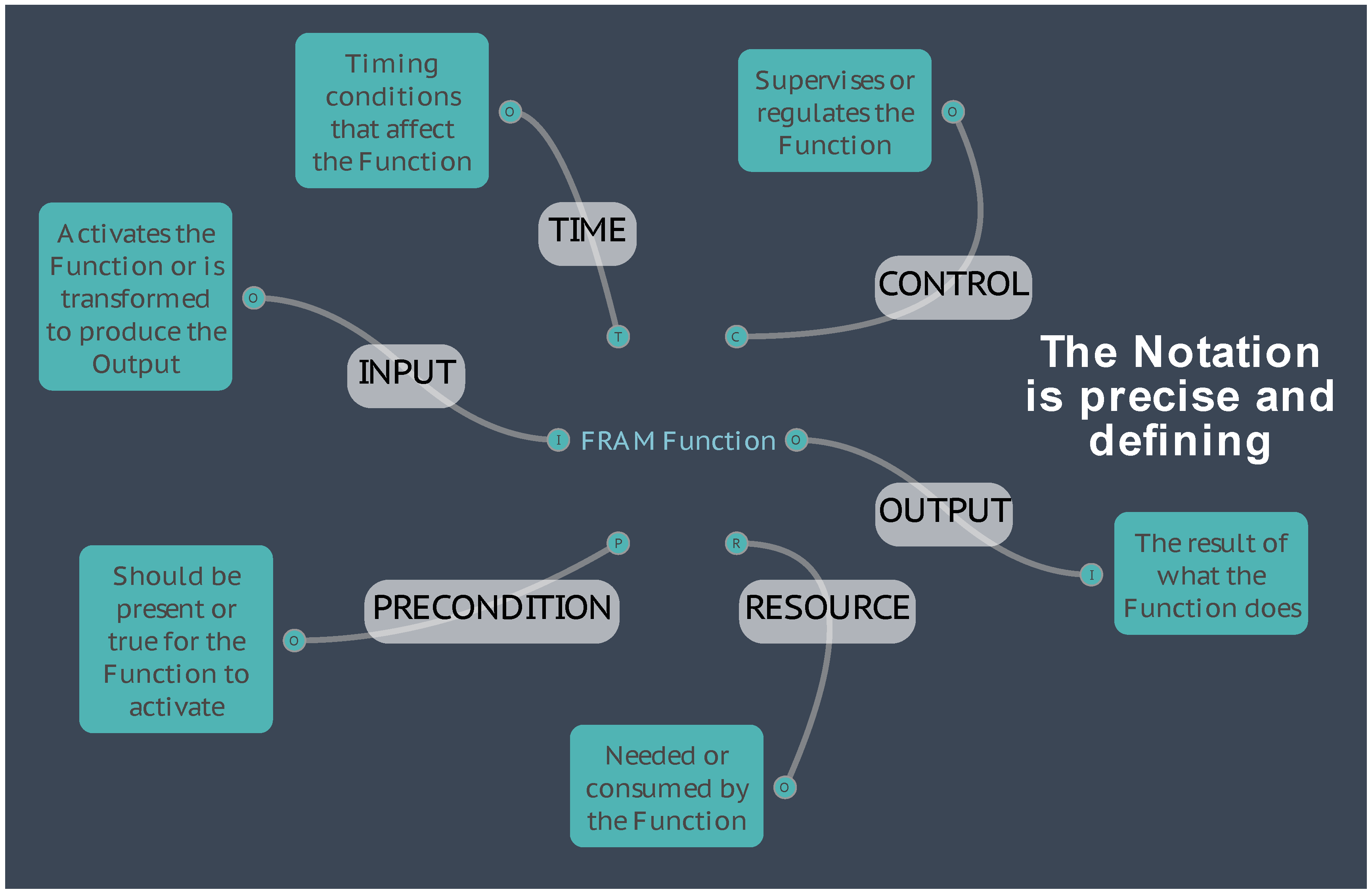
The FRAM Model Visualiser
3.2. Current Applications of the Method
3.3. The Further Development of the Methodology
3.3.1. Variability
- MyFRAM, was developed by Patriarca (2017) and used as a powerful pre- and post- processor by various researchers, where an FMV data file could be read into the application and the data could be viewed and edited in spreadsheet views, including calculations and other qualitative or quantitative analysis of variabilities to predict resonances. The resulting model could be output as an FMV data file to be displayed again in the FMV software. (for example, Patriarca’s MonteCarlo application).
- Early on in the FMV development, a successful integration was made (Slater (2017)) to pass data to an external Bayesian Belief Network (BBN) processor, using the open source i-Depend software, returning results to the FMV for visualisation.
- Another example of quantitative post-processing employed a Fuzzy Logic approach (Takayuki (2019), that manipulated FMV Functional properties (Metadata see 3.2.2.3) in an external program, creating an output that could be displayed and visualised in the FMV application. Variability was represented by a Degree of Variability (DoV) property of a Function, modified by couplings with other Functions.
3.3.2. Validation
A production system (or production rule system) is a computer program typically used to provide some form of artificial intelligence, which consists primarily of a set of rules about behaviour, but it also includes the mechanism necessary to follow those rules as the system responds to states of the world.
3.3.3. Purposes of the FMI
-
One purpose of the FMI is to check whether the model was syntactically correct.
- -
- An important part of that is the identification of “orphans”, (i.e., unconnected aspects), that the FMV already provides as a visual check. To begin the FMI interpretation, all defined aspects must connect to other functions as potential couplings.
- -
- Other problems that the FMI flags as invalid, are potential auto-loops, where the Output from a Function is used directly by the Function itself. The FMV however, will not make this type of connection and flags it as an orphan.
- -
- Finally, there is a check on the Inputs and Outputs by FMI Function Type. If a Function has aspects apart from Inputs and Outputs, then it is, by definition, a foreground Function and it must have at least one Input and one Output.
- A second purpose of the FMI was to understand the difference between potential and actual couplings among Functions. A FRAM model describes the potential couplings among Functions, i.e., all the possible ways Functions are related as specified by their aspects. In contrast to that, the actual couplings are the upstream-downstream relations that occur when an activity is carried out, which means when the FRAM model is realised for a set of specified conditions. (a so-called instantiation).
- A third purpose was to determine whether the activity described by the model will, in fact, develop in practice. In a FRAM model each foreground Function defines a set of upstream-downstream relations through its aspects. The question is whether these relations are mutually consistent and whether they in fact will allow an event to develop as intended.
- It is all too easy in a complicated model, to have Functions that mutually depend on each other, which in practice may lead to conditions where Functions wait forever for an aspect to become fulfilled. The FMI can identify these cases by interpreting the model step-by-step while keeping track of the status of all the aspects and activation conditions.
- A further purpose is to investigate the consequences of variability of Functions. In the Basic FMI this is done indirectly, by specifying the conditions under which a Function may become activated, rather than by considering the variability of outputs directly.
3.3.4. Metadata
3.3.5. Dynamics
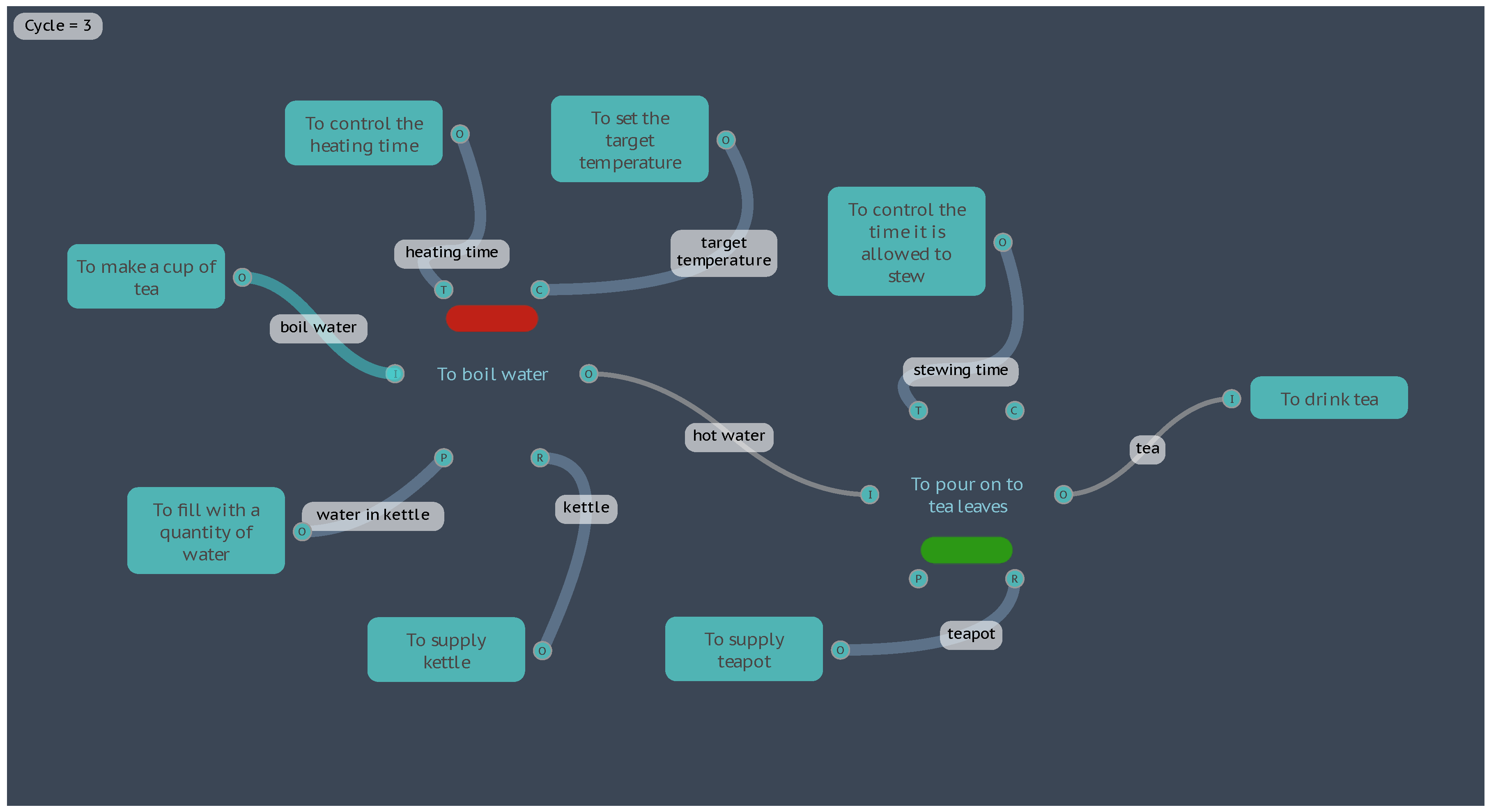
- The activation of the Entry Function(s) on the initial Cycle 0 of the FMI can be repeated at a set cycle interval, effectively pulsing the model.
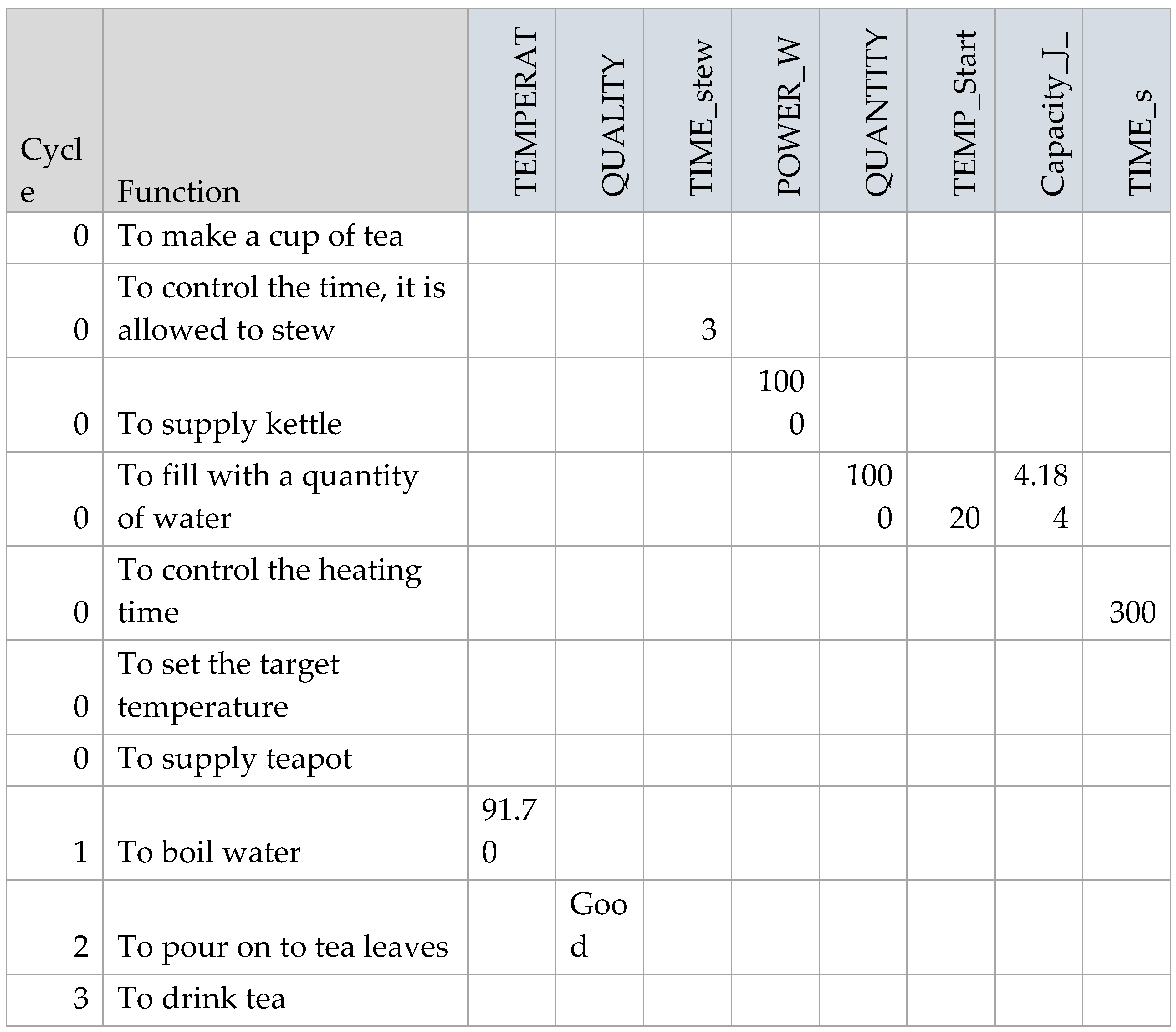
- The FMI interpretation can be extended beyond the default stop conditions (when all Exit Function(s) have activated) for a set number of cycles, or continuously until manually stopped.
- An equation can be added to the FMI Profile to consider the aspects and their Metadata in more detail, before an Output is produced, potentially putting a Function on ‘Hold’ until conditions are met on a subsequent cycle.
- A table of lookup values can be referenced by the equations.
4. How It Works
4.1. Detailed Description of Metadata in FRAM
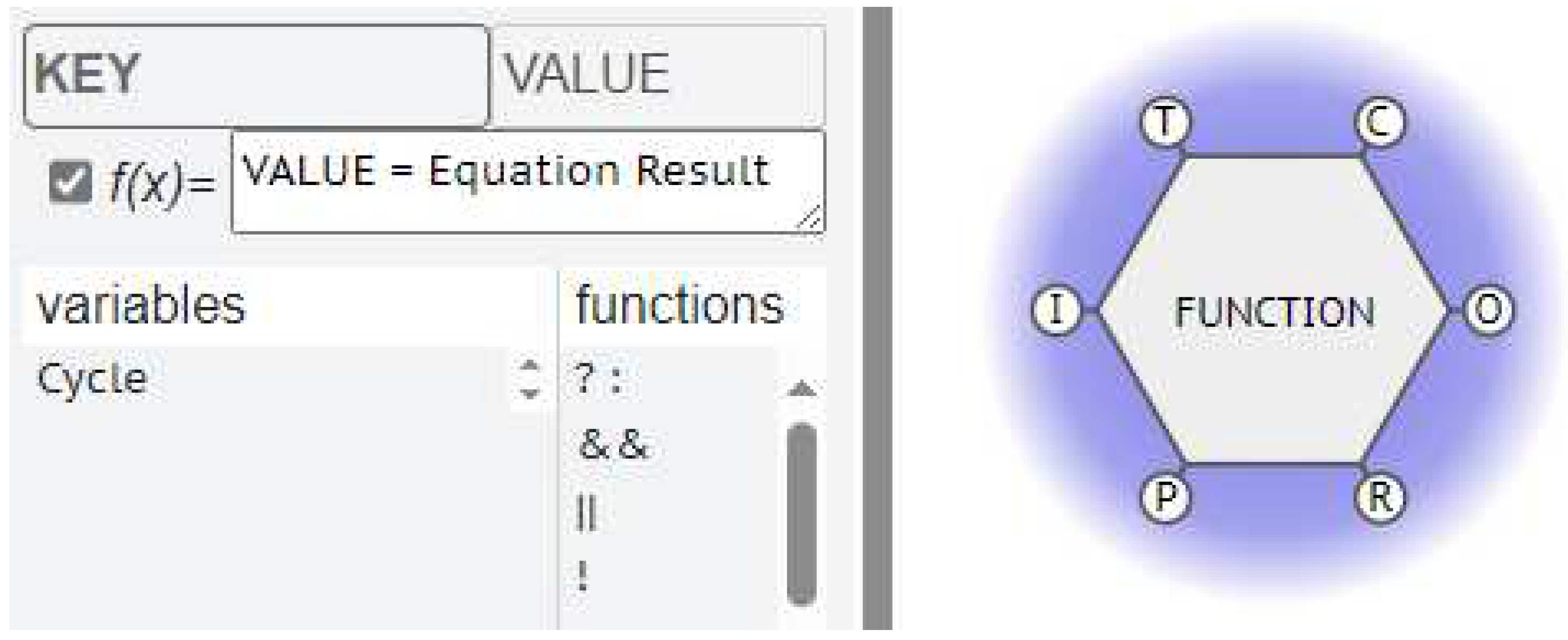
- Fixed constants that represent properties of a specific Function, like a name, description, or other properties.
- Variable properties of a specific Function that can be modified using equations based on other metadata available from upstream Functions.
- Global constants that are set by the starting Function and passed on through the couplings.
- Global variables that are passed on through the couplings but can be modified by Functions using equations as they pass through.
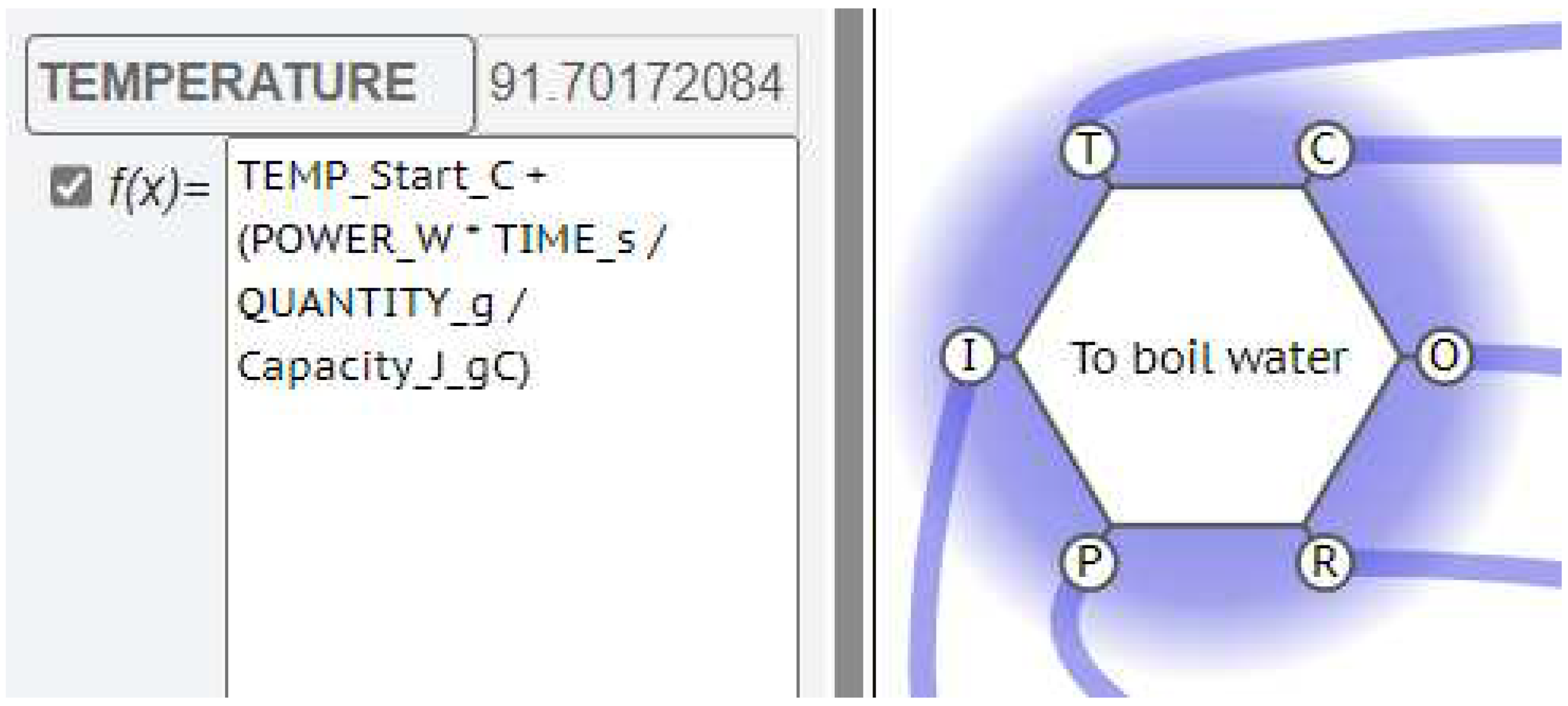
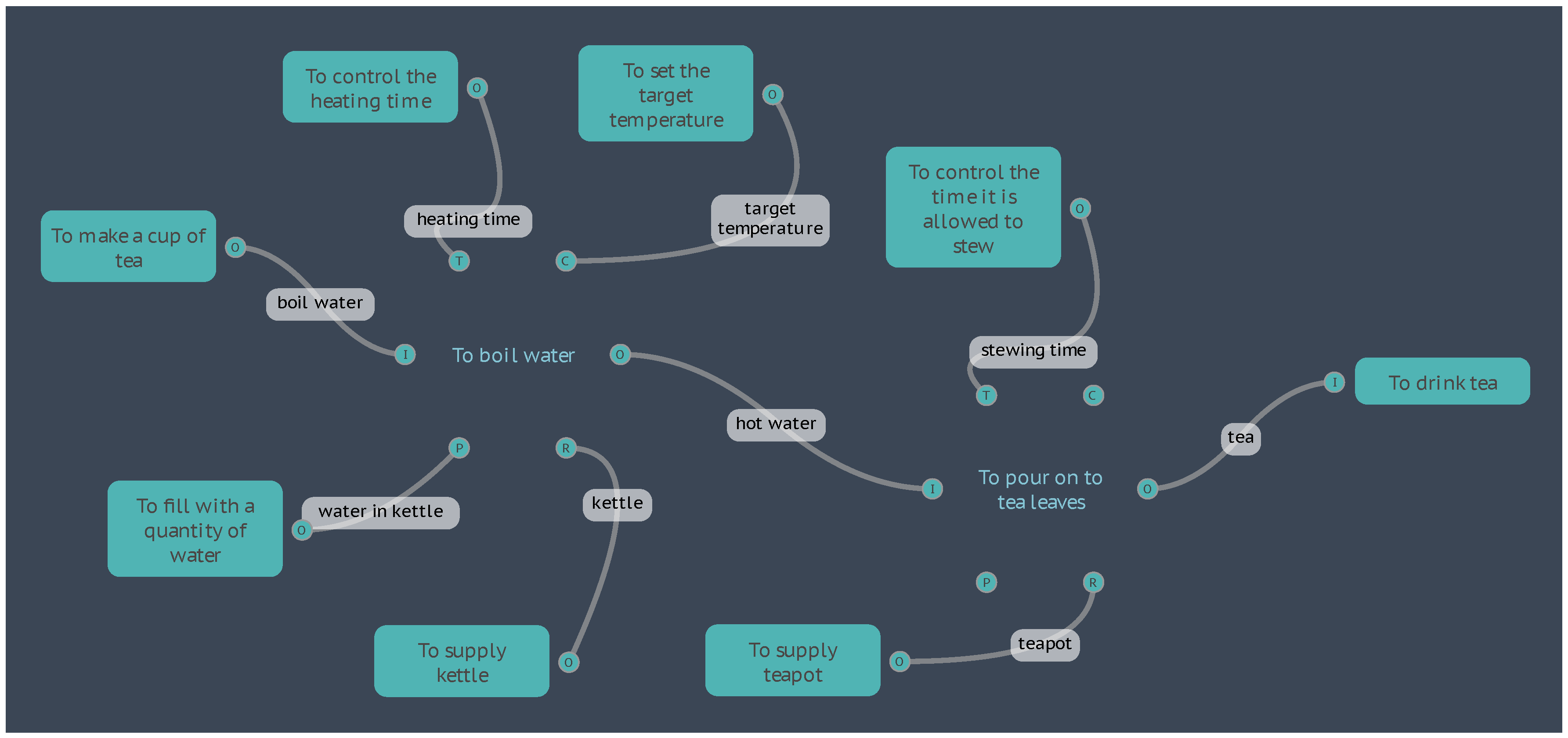
4.2. Examples of Metadata
4.2.1. Boil Water
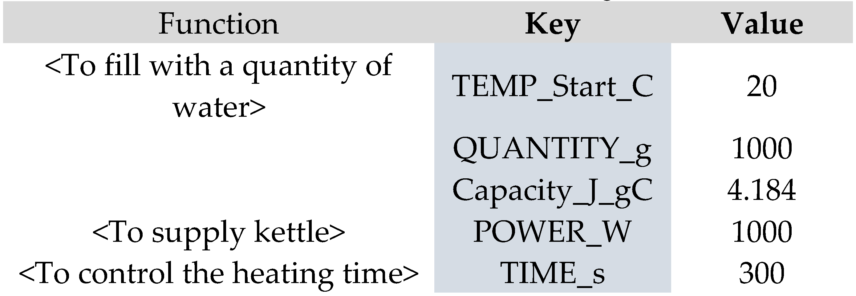
- TEMP_Start_C is the starting temperature of the water in degrees Celsius (°C)
- POWER_W is the power rating of the electric kettle in Watts (W), which is the same as Joules per second (J⋅s-1)
- TIME_s is the time that the water is allowed to heat, in seconds (s)
- QUANTITY_g is the quantity of the water that is being heated, in grams (g)
- Capacity_J_gC is the specific heat capacity of water, at 4.184 Joules per gram, per degree Celsius (J⋅g-1⋅°C-1)
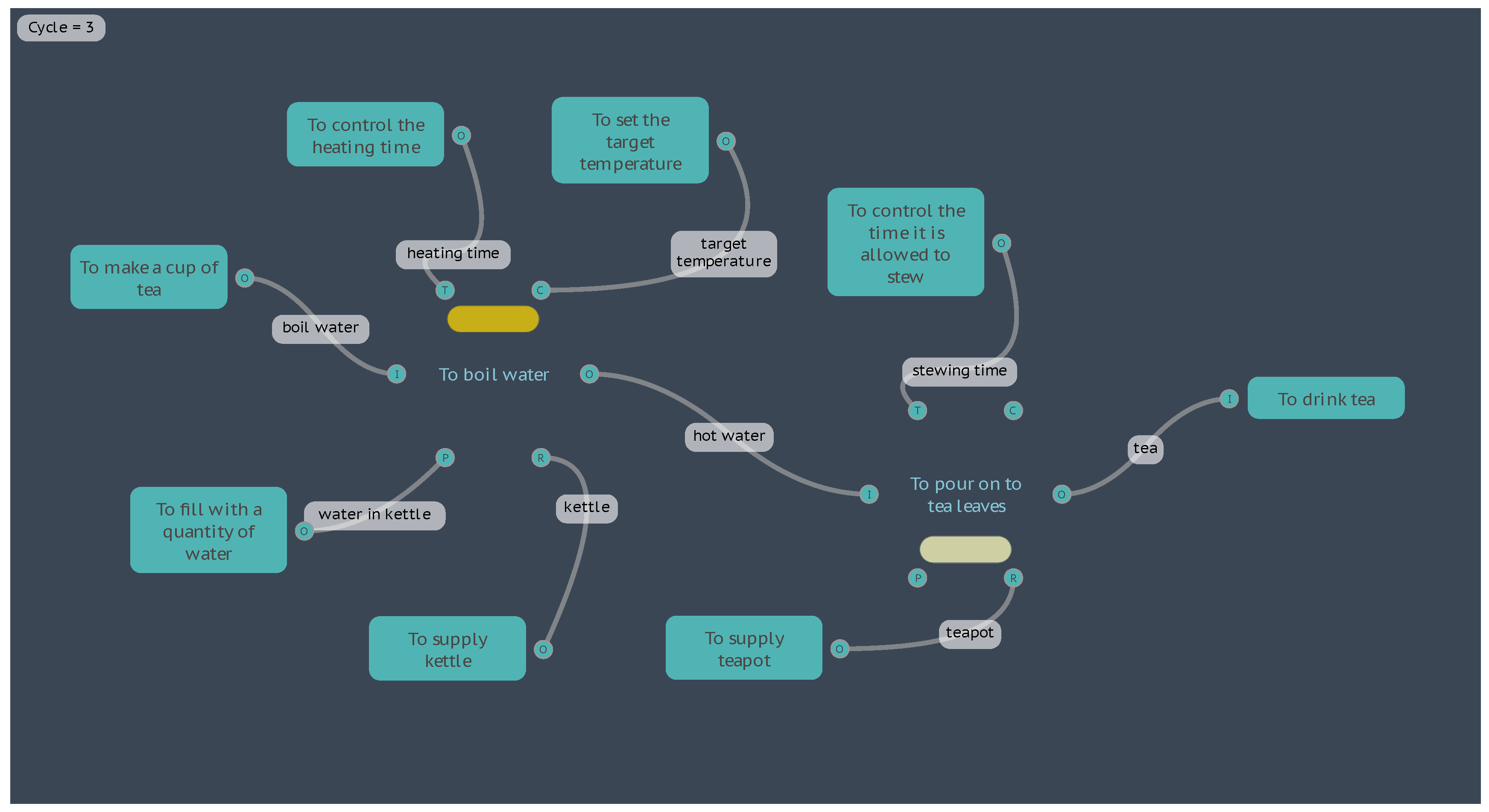
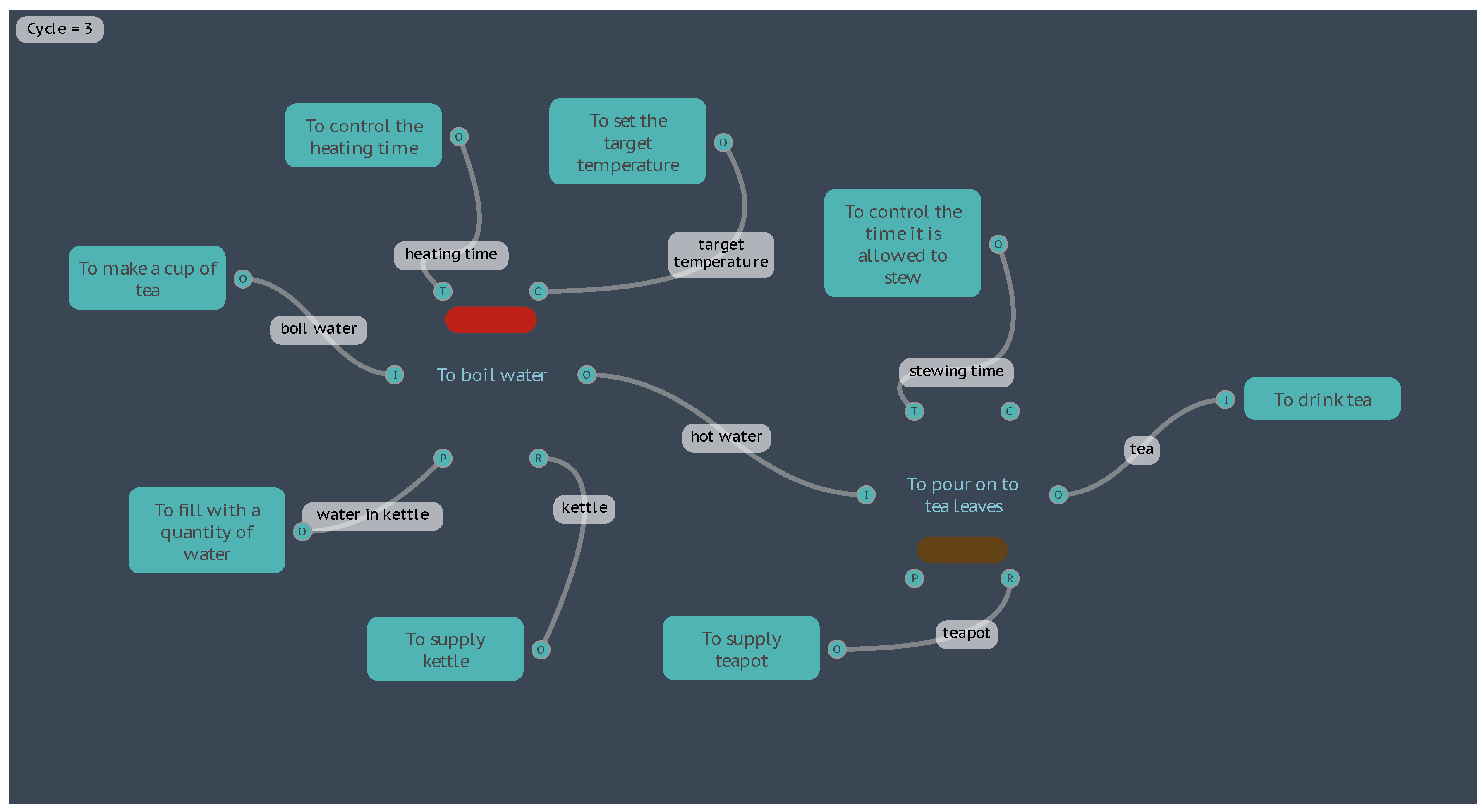
- 1.
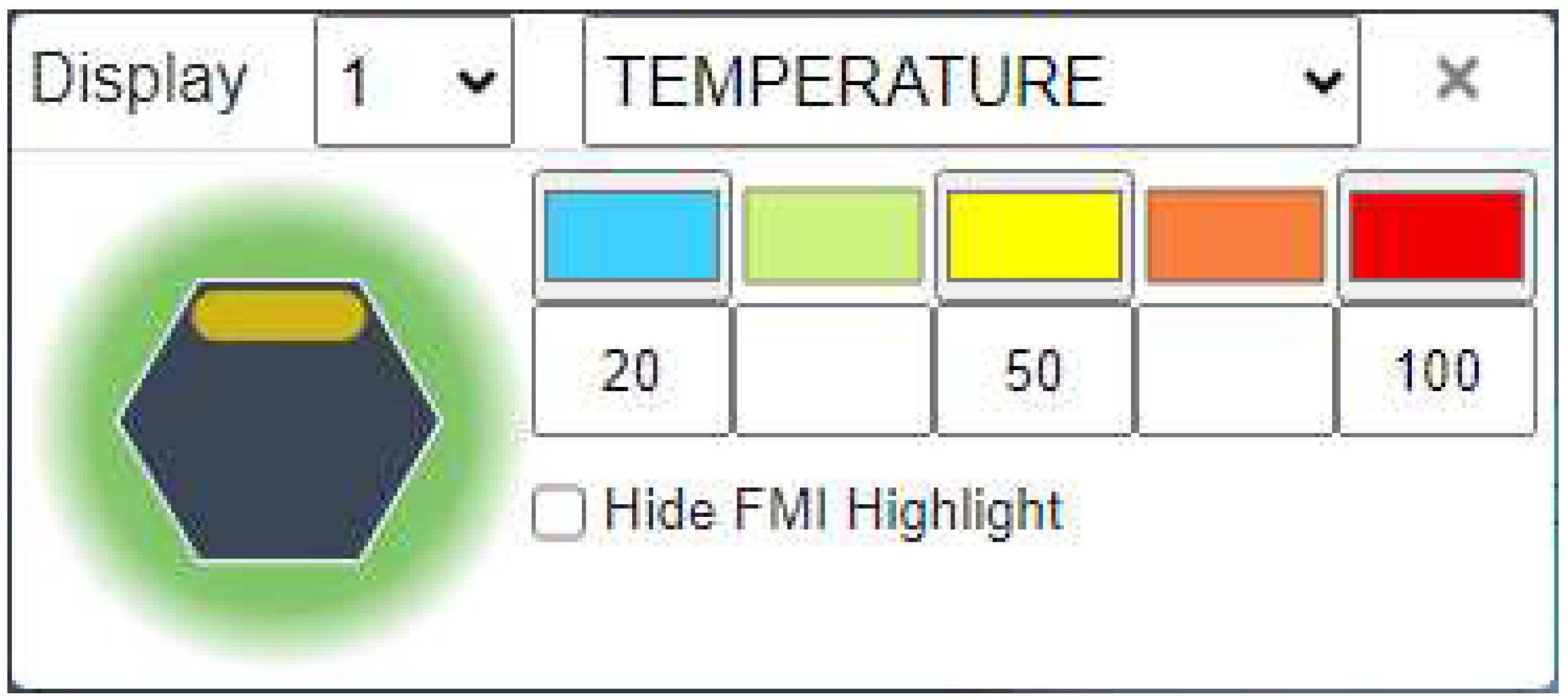
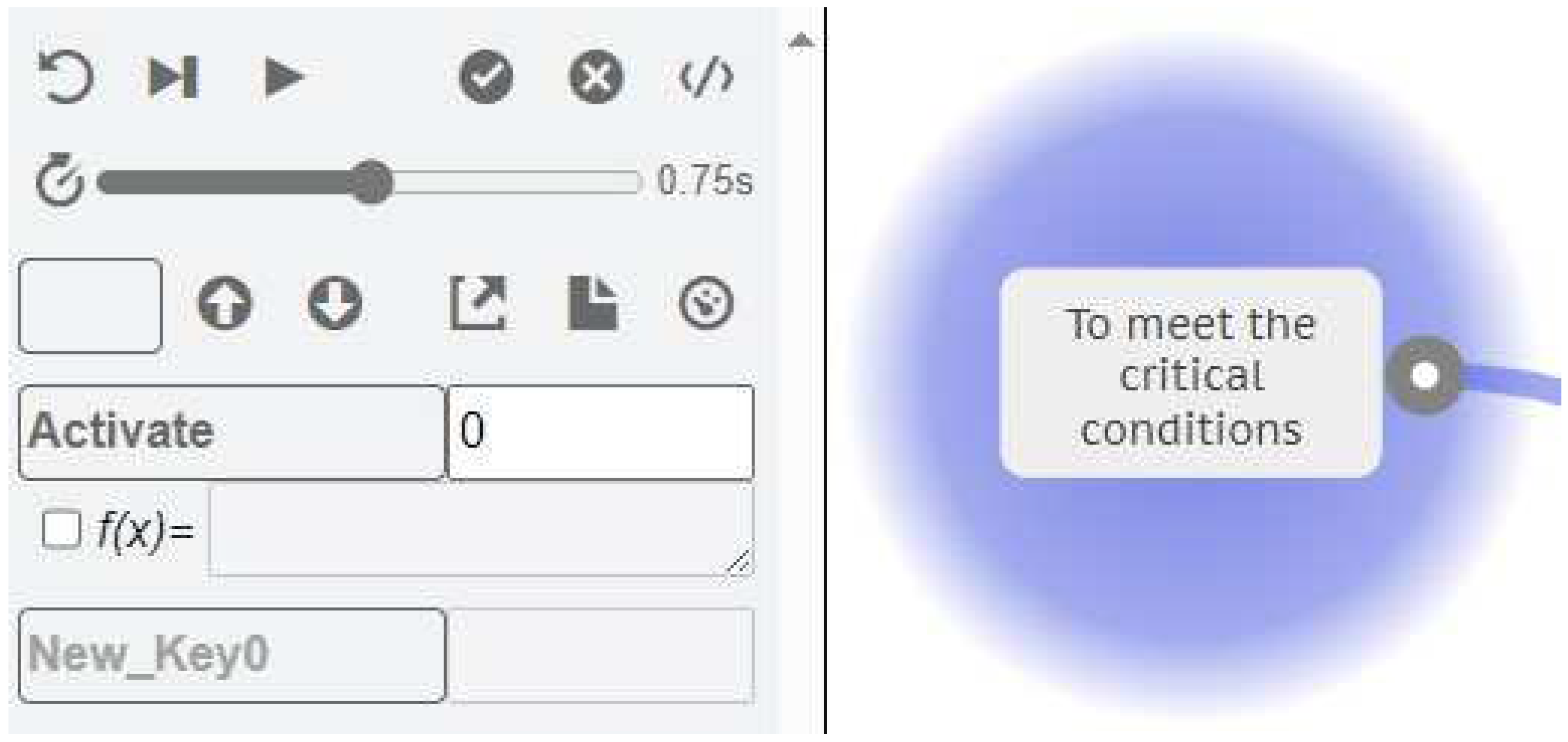
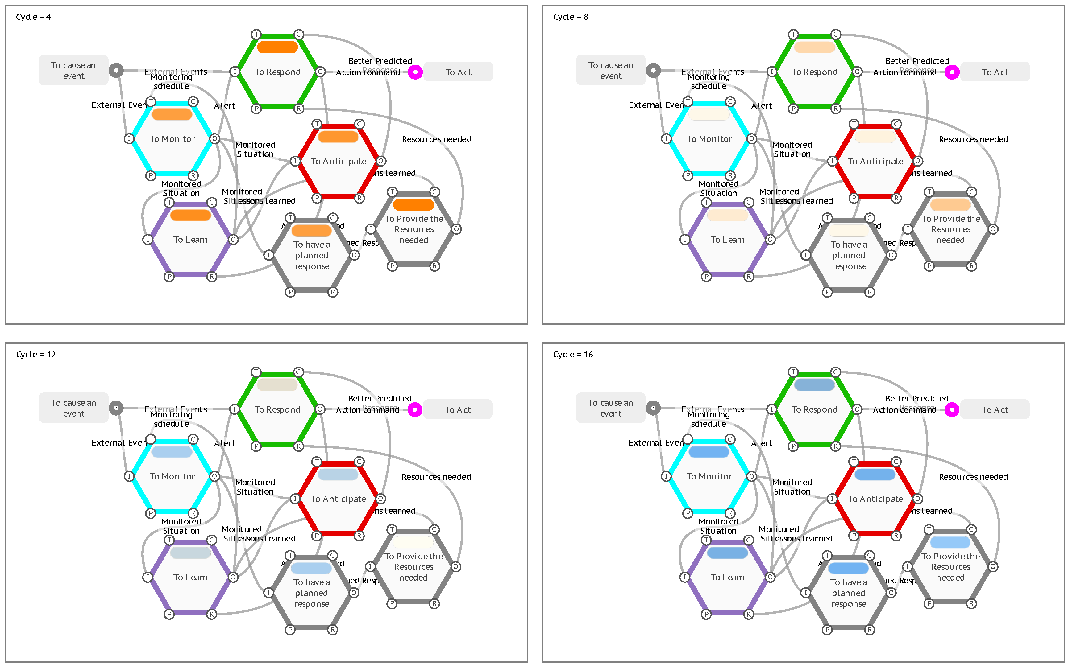
- For the Metadata key TEMP_Start_C on the Function <To fill with a quantity of water>, the value can be changed to 0, to set the starting point for the first instantiation, and then an equation added, where TEMP_Start_C = TEMP_Start_C + 1. This will start with 0°C and increase the temperature by one degree every instantiation.
- 2.
- The equation can be set to a pseudo-random number within a given range. For example, to start an instantiation with a random integer between 10 and 30 (inclusive), the equation would be TEMP_Start_C = rndi(10,31). Double precision floating point numbers can also be generated using rnd().
- 3.
- The equation can be set to return a pseudo-random number that, on repetition, approximates a normal distribution. For example, a normal distribution with a mean of 20 and a standard deviation of 10 would be TEMP_Start_C = rnorm(20,10)
- 4.
- A table of values can be imported into the model, and an equation used to return a value from the table, such as lookup(row number,column number). In our example, the row number can be set from the available system variable that contains the current Cycle number, Cycle, and the first column of the data table, such that: TEMP_Start_C = lookup(Cycle/3,0)
- 5.
- Similar to the previous case, a value can be referenced from a data table, but using a cross reference between a row name contained in the first column, and returning data from another column referenced by a column header name, such as TEMP_Start_C = xref(Cycle,”Temp”). In this case the data table does not need to be sorted or sequential.
4.2.2. Plan A or Plan B
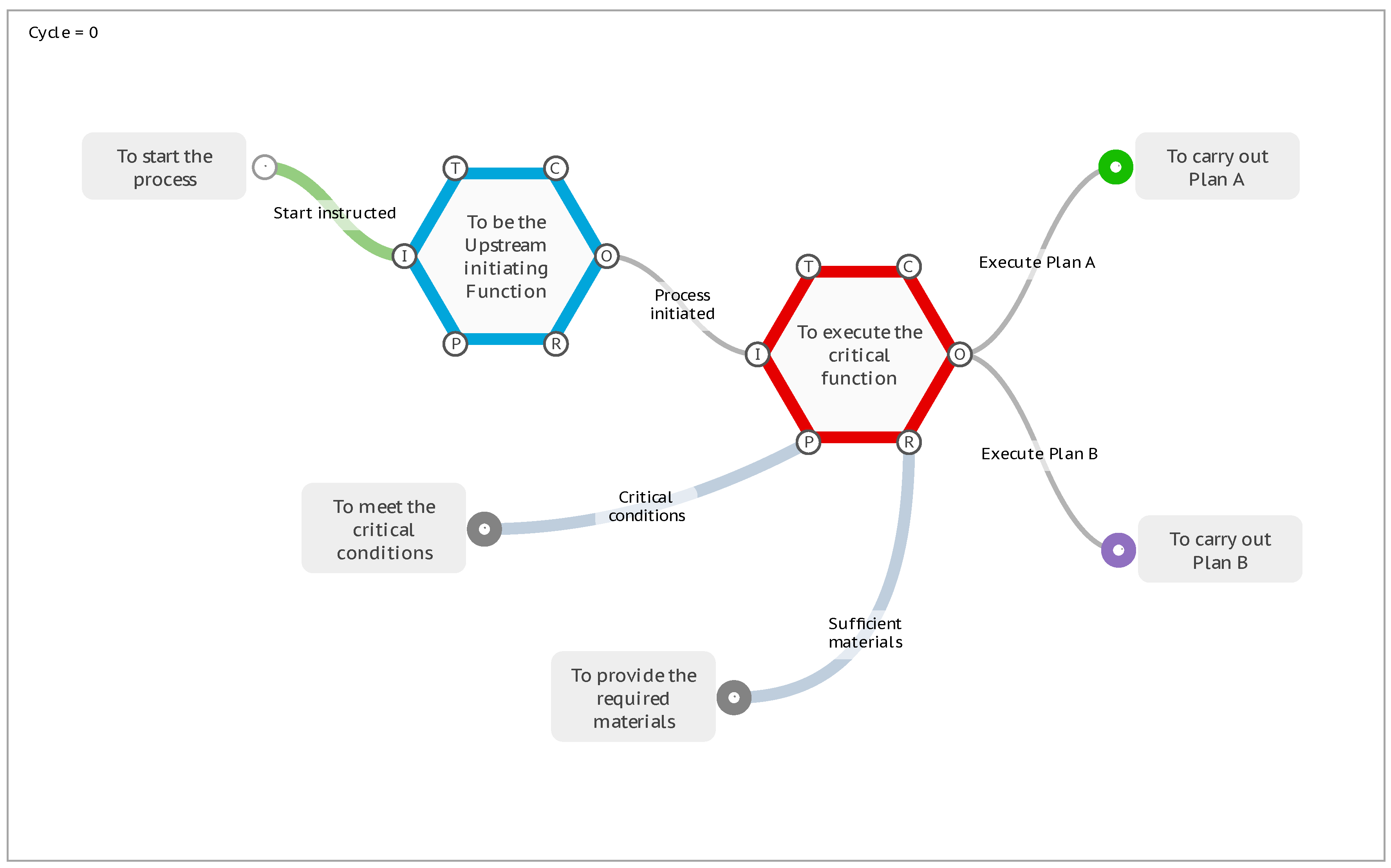
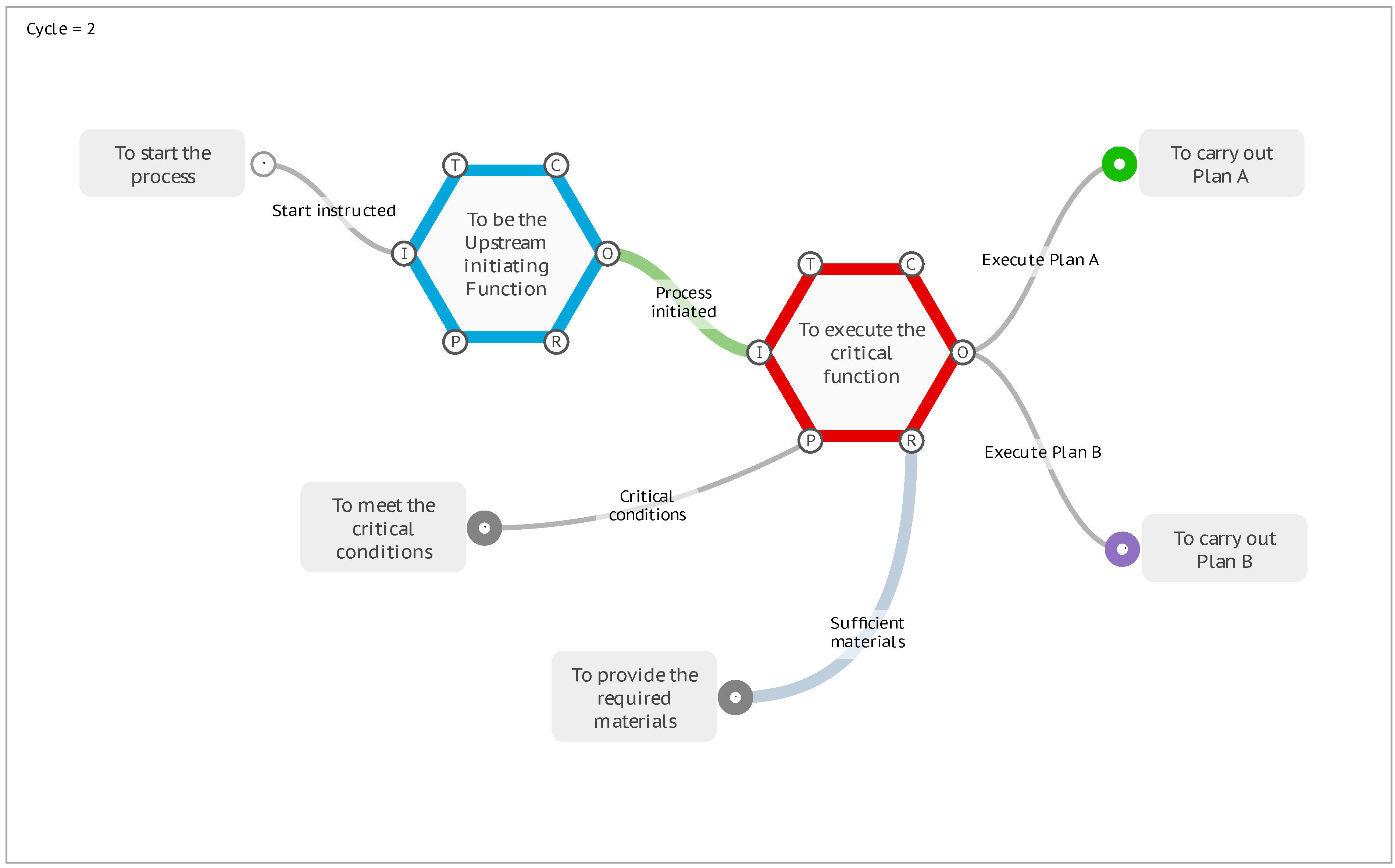
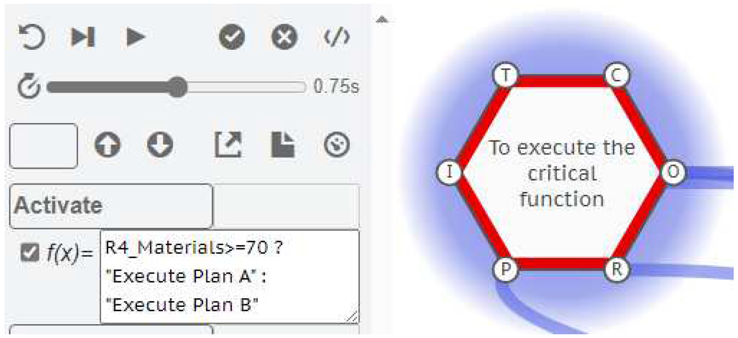
4.2.3. Resilience Potentials
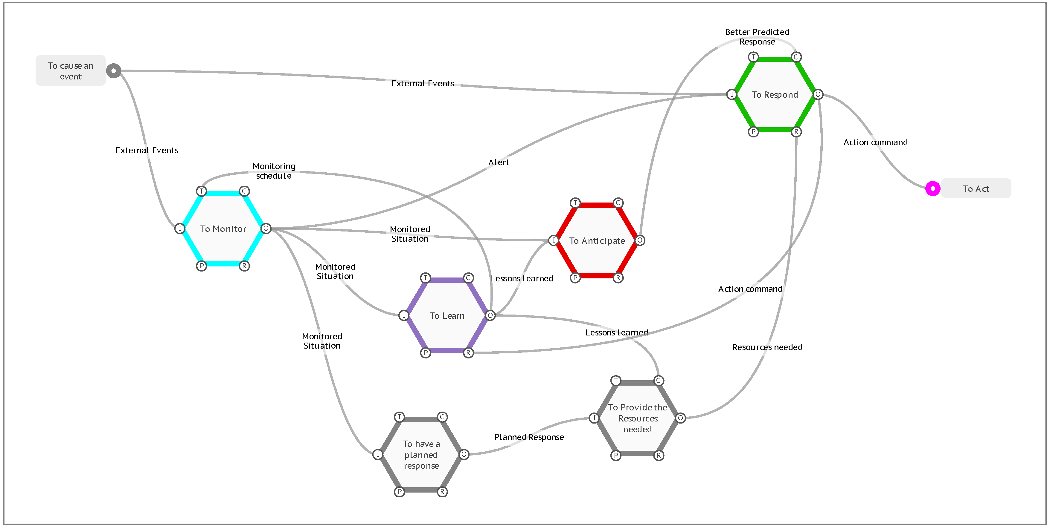
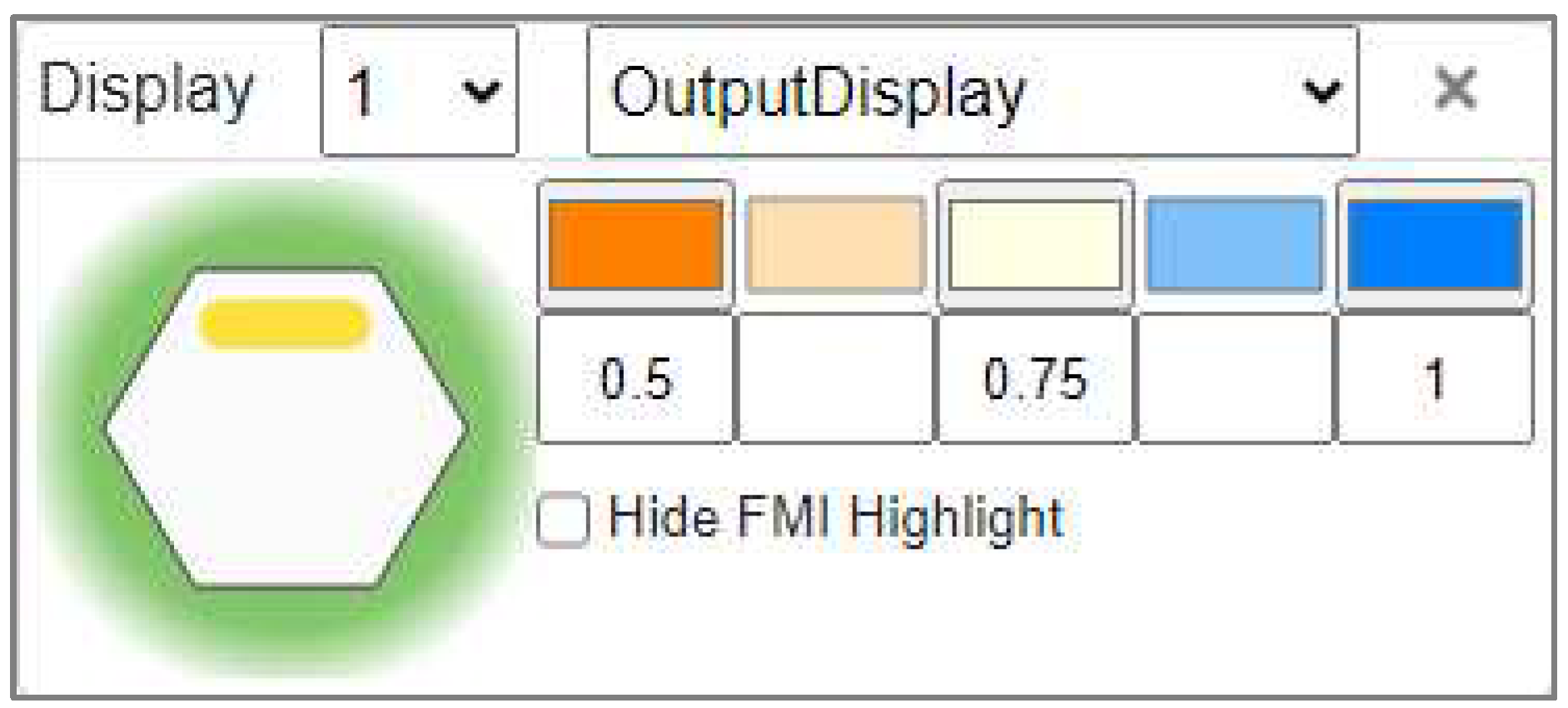
4.3. Current Applications of the Metadata
4.3.1. Formula 1 Pit Stop
4.3.2. Patient Management / Safety
5. Discussion
5.1. The Current Utility of the Approach
5.2. Further Possibilities Made Feasible.
- Human – Human systems (Shiota (2023)
- 6.
- Human robot systems (Warehouses, robotic surgery (Adriaensen, (2023))
- 7.
- Self-driving cars (Grabbe) Auto-autos (Grabbe 2023)
- 8.
- Machine Learning (Nomoto (2023))
- 9.
- Software system safety and security – AI? (Thurlby (2023)
5.3. The Future
5.3.1. Process Simulation
5.3.2. Digital Twins
6. Conclusions
Author Contributions
Funding
Acknowledgments
Conflicts of Interest
| 1 | |
| 2 | INCOSE SE Vision 2020 (INCOSE-TP-2004-004-02, Sep 2007) OMG /) |
| 3 | The GitHub URL is https://github.com/functionalresonance
|
| 4 | Each stage of FMV software development was reviewed with Erik Hollnagel to ensure that the software always supported the original method and helped lead to its wide use and acceptance in teaching the FRAM method and visualising FRAM models. |
| 5 |
References
- Abubakar, A; Bagheri Z, P; Janicke, H; Howley, R, (2016). "Root cause analysis (RCA) as a preliminary tool into the investigation of identity theft". Proc. 2016 International Conference On Cyber Security And Protection Of Digital Services (Cyber Security).
- Ackoff, R, (1968), "General Systems Theory and Systems Research Contrasting Conceptions of Systems Science." in: Views on a General Systems Theory: Proceedings from the Second System Symposium, Mihajlo D. Mesarovic (Ed.).
- Adriaensen, A, (2023), Development of a Systemic Safety Assessment Method for Human-Robot Interdependencies, Dissertation presented in partial fulfilment of the requirements for the degree of Doctor of Engineering Science (PhD): Mechanical Engineering, KU Leven.
- bar Yam, Y. McKay, S and Wolfgang C. (1998) Dynamics of Complex Systems (Studies in Nonlinearity) Computers in Physics 12(4):335–336. [CrossRef]
- Booch, G, (1993). Object-oriented Analysis and Design with Applications (2nd ed.). Redwood City: Benjamin Cummings. ISBN 0-8053-5340-2.Marca, D. McGowan, C, Structured Analysis and Design Technique, McGraw-Hill, (1987), ISBN 0-07-040235-3.
- Box, G. E. P.; Draper, N. R. (1987), Empirical Model-Building and Response Surfaces, John Wiley & Sons.
- Coombs, Dawes, & Tversky, (1970), Mathematical Psychology: An Elementary Introduction, Prentice-Hall, 1970 - Psychology - p. 2.
- Franca, J. and Hollnagel, E. (2020), Safety-II Approach in the O&G Industry: Human Factors and Non-Technical Skills Building Safety, Rio Oil & Gas Expo and Conference 2020, ISSN 2525-7579 Conference Proceedings homepage: https://biblioteca.ibp.org.br/riooilegas/en/.
- Goldberg, B. E.; Everhart, K.; Stevens, R.; Babbitt, N.; Clemens, P.; Stout, L. (1994). "3". System engineering toolbox for design-oriented engineers. Marshall Space Flight Centre. pp. 3–35 to 3–48.
- Grabbe, N. (2023), Assessing the reliability and validity of an FRAM model: the case of driving in an overtaking scenario, FRAMily 2023, Copenhagen, https://functionalresonance.com/framily-meetings/FRAMily2023/Presentations/FRAMily_Copenhagen_2023_Grabbe.pdf. [CrossRef]
- Hill, R, (2016) in Hollnagel, E. The way ahead: FRAM extensions and add-ons, FRAMily 2016 Lisbon, https://functionalresonance.com/onewebmedia/FRAMtid_2.pdf (retrieved 1/11/2923).
- Hollnagel, E, (2012), FRAM: The Functional Resonance Analysis Method, Modelling Complex Socio-technical Systems, CRC Press, London,. [CrossRef]
- Hollnagel, E, (2021) The FRAM Model Interpreter, FMI, https://safetysynthesis.com/onewebmedia/FMI_Plus_V2-1.pdf.
- Hollnagel, E, (2022), Systemic Potentials for Resilient Performance, chapter In book: Resilience in a Digital Age, . [CrossRef]
- Hopkins, A, (2000), Lessons from Longford: The Esso Gas Plant Explosion, CCH.
- IEC; ISO (2019). Risk Management – Risk Assessment Techniques. IEC 31010 (2.0 ed.). Geneva: International Electrotechnical Commission. ISBN 978-2-8322-6989-3.
- Leveson, N, (2004) IEC; ISO (2019). Risk Management – Risk Assessment Techniques. IEC 31010 (2.0 ed.). Geneva: International Electrotechnical Commission. ISBN 978-2-8322-6989-3.
- MacKinnon, R, et al, (2023), MacKinnon R, Barnaby J, et al., 2023. Adding Resilience to Hospital Bed Allocation, using FRAM, Medical Research Archives, [online] 11(10). [CrossRef]
- Nomoto, H. et al, (2023), Machine Learning in FRAM, FRAMily 2023, Copenhagen, https://functionalresonance.com/framily-meetings/FRAMily2023/Presentations/MLforFRAM.pdf.
- Nomoto, H. et al (2022), Bayesian FRAM, FRAMily 2022, Kyoto, https://functionalresonance.com/framily-meetings/FRAMily2022/Files/Presentations/3_2_2_BaysianFRAM_Nomoto.pdf.
- Patriarca, R, et al., (2020) Framing the FRAM: A literature review on the functional resonance analysis method Safety Science 129:104827Follow journal. [CrossRef]
- Patriarca, R. (2017) myFRAM: An open tool support for the functional resonance analysis method, Conference: 2017 2nd International Conference on System Reliability and Safety (ICSRS), DOI: 10.1109/ICSRS.2017.8272861.
- Perrow, C. (1984), Normal Accidents: Living with High-Risk Technologies New York: Basic Books, p.5.
- Rasmussen J (1997) Risk management in a dynamic society: a modelling problem. Saf Sci 27(2):183–213.
- Rausand, M; Høyland, A, (2004). System Reliability Theory: Models, Statistical Methods, and Applications (2nd ed.). Wiley. p. 88.
- Reason, J (1990). "The Contribution of Latent Human Failures to the Breakdown of Complex Systems". Philosophical Transactions of the Royal Society of London. Series B, Biological Sciences. 327 (1241): 475–84. Bibcode:1990 RSPTB.327..475R. doi:10.1098/rstb.1990.0090. JSTOR 55319. PMID 1970893. [CrossRef]
- Selfridge, O. G. (1958). Pandemonium: a paradigm for learning. In: Mechanism of Thought Processes. Proceedings of a Symposium Held at the National Physical Laboratory. (p.513-526.).
- Shota Iino, Hideki Nomoto, Takayuki Hirose, Yasutaka Michiura, Yumi Ohama, Maria Harigae (2023) Revealing success factors of cooperative operations in space manned missions: crucial factors in Apollo missions, FRAMily 2023, Copenhagen.
- Slater, D. (2016) Open Group Standard Dependency Modelling (O-DM), DOI: 10.13140/RG.2.1.1150.7445, https://www.researchgate.net/publication/305884742_Open_Group_Standard_Dependency_Modeling_O-DM.
- Slater, D, et al (2021) Optimising the Performance of Complex Sociotechnical Systems in High-Stress, High-Speed Environments: The Formula 1 Pit Stop Test Case, Appl. Sci. 2021, 11, x. [CrossRef]
- Smith, D, et al. (2022) The Functional Resonance Analysis Method as a health care research methodology: a scoping review;20(4):1074-1097. [CrossRef]
- Snowden, D J.; Boone, Mary E. (2007). "A Leader's Framework for Decision Making". Harvard Business Review. 85 (11): 68–76. PMID 18159787.
- Takayuki, H, et al. (2023) FRAM: The Development of the Complex System Analysis Methodology, https://www.researchgate.net/publication/372079036_FRAM_The_Development_of_the_Complex_System_Analysis_Methodology.
- Thurlby, J. (2023), THE ILLUSION OF SAFETY: AVOIDING SAFETY THEATRE IN AUTOMOTIVE SOFTWARE DEVELOPMENT, https://www.linkedin.com/pulse/illusion-safety-avoiding-theater-automotive-software-joel-thurlby/.
- Williams, S. (1967) "Business Process Modelling Improves Administrative Control," In: Automation. December 1967, pp. 44 - 50.
Disclaimer/Publisher’s Note: The statements, opinions and data contained in all publications are solely those of the individual author(s) and contributor(s) and not of MDPI and/or the editor(s). MDPI and/or the editor(s) disclaim responsibility for any injury to people or property resulting from any ideas, methods, instructions or products referred to in the content. |
© 2024 by the authors. Licensee MDPI, Basel, Switzerland. This article is an open access article distributed under the terms and conditions of the Creative Commons Attribution (CC BY) license (http://creativecommons.org/licenses/by/4.0/).


