
Submitted:
02 February 2024
Posted:
02 February 2024
You are already at the latest version
Abstract
Space instable target simulator (SITS) is a vital actuator for ground verification of on-orbital capture technology, the motion performance of which directly affects simulation credibility. Different delays reduce the stability of SITS and ultimately lead to its divergence. In order to achieve high fidelity simulation, the impact of force measurement delay, discrete control cycle, and simulator response delay on stability is analyzed firstly. Then, the dynamic equation and transfer function identification model of hybrid simulator is constructed, and the necessary and sufficient conditions of its stability and convergence are obtained using the Routh criterion. After that, a switching compensator with variable gain is proposed, the compensation principle diagram of which is build, and its mathematical model including the energy observer and tracking differentiator is also established. Finally, three sets of numerical simulations are conducted to validate the correctness of the stability analysis and effectiveness of proposed compensation method. Simulation results show that all three types of delay can cause SITS to lose stability under critical stable motion state, and the delay in force measurement has the greatest impact, followed by the influence of control cycle. Compared with the force applied to simulated target, velocity and its recovery coefficient of space instable target using fixed gain and linear gain compensation, the proposed compensator has significantly better performance.
Keywords:
space instable target
; stability analysis
; delay compensation
; hybrid simulator
; switching compensator with variable gain
1. Introduction
With the increase in human space activities, the number of non-cooperative space objects such as defunct satellites and spacecraft debris continues to rise, significantly impacting the utilization of orbital resources and the space operational environment [1,2,3]. Active debris removal (ADR) technology involves the use of tools like robotic arms to repair and clean up space debris, effectively reducing the generation of space debris. This technology proves instrumental in mitigating the threats posed by uncontrolled debris in the space environment and alleviating congestion in orbital space [4,5,6,7].
Direct on-orbit application of ADR technology poses significant risks, generally necessitating comprehensive ground tests to address shortcomings in technical methods and validate the stability. Full physical simulation (FPS), semi-physical simulation (SPS), and digital simulation (DS) are currently the three commonly applied ground experiment approaches. Full-sized simulators with complete physical characteristics are typically constructed in FPS, which incurs high costs. In addition, it is difficult to achieve frictionless movement along the direction of gravity in the simulation of 6-DoF spatial weightlessness motion [8,9,10]. DS, not reliant on physical hardware, conducts verification of debris removal processes only through mathematical modeling [11,12,13]. The mathematical model for actual contact process cannot be accurately established, and it also lacks the capability to optimize and improve the real capture tool, presenting certain limitations. SPS combines the advantages of FPS and DS, incorporating vital physical hardware into the test system to reduce the unnecessary costs of hardware [14,15,16,17,18]. Simultaneously, it utilizes mathematical spacecraft models with different mass and inertia characteristics, making it widely applied in ground experiments for space mechanism.
The ground capture SPS system for space instable target (SIT) is a system with high real-time requirements. SITS is a critical device, and its motion performance is directly related to the accuracy of the simulation. Delays have significant effects on the stability and precision of SPS system, leading to invalid test data or even damage of simulator due to instability.
Researches on the reasons and compensation methods for the delay of simulator in SPS system have gained certain progress. M. Zebenay et al. [19] addressed the response time delay of the industrial robot controller in the European Proximity Operations Simulator (EPOS 2.0 c) and the impact of robot high stiffness on the safety and the authenticity of experiment results. A contact collision model suitable for ground verification is proposed, combining impedance control with mechanical passive compliance, which builds the relationship between robot stiffness and test device stiffness. Based on estimating contact stiffness and damping, M. Zebenay introduced compensation into the dynamic model to achieve 1D hybrid simulation in 2015 [20]. By comparing the maximum contact force and velocity recovery coefficient of 1D movement with an air-floating test system, the feasibility of hybrid simulator was verified. Aiming at response delay of the 6-DoF parallel mechanism in ground SPS platform, Chenkun Qi [21] investigated a real-time online identification method for contact stiffness, which was estimated through differential equations based on force, displacement, and velocity within three contact cycles. Adopting this information as the compensation of dynamic input, system divergence was suppressed with achieving a velocity recovery coefficient of 0.9809. To address the issues of system instability and simulation distortion caused by time delay and discrete integration of dynamics in the On Orbit Servicing Simulator loop, Marco De Stefano [22] proposed a passive controller for adjusting admittance dynamics input force and a speed modulation controller for maintaining energy characteristics. The instability suppression effect in satellite dynamics reproduction was verified on industrial robots. LAV Sanhith Rao [23] analyzed the motion divergence caused by the delay in the three-axis rotational semi-physical test platform for aerospace products. By compensating for the turntable angular velocity based on establishing the system transfer function, they successfully solved the undesired oscillations and inaccurate experiment results. The reason for the increase of system energy was identified through analyzing the phase relationship between force and velocity in complex domain by Kohei Osaki [24]. The force compensation model is established and applied to 1D collision experiments, achieving a recovery coefficient of 0.97 with satisfactory results. However, due to neglecting the velocity phase variation caused by force lag, this mean provides an approximate compensation effect. Satoko Abiko [25] presented a force compensation way based on the velocity recovery coefficient. By observing the velocity change online, they identified the compensation coefficient for input force of dynamic model and applied it to the planar 3-DoF collision tests.
There is a considerable risk to identify stiffness and damping in real-time during actual capture process and the feasibility is weak, especially when the contact stiffness is high, that is, the contact time is also rather short. Moreover, relying solely on adjusting the impedance characteristics of manipulator to indirectly extend the contact time and suppress divergence is not a fundamental approach to solve the divergence issue of simulator. The integral lag in dynamics is just one aspect of control cycle delay. Only settling this problem while neglecting other lag impacts leaves the simulator in a divergent state. Similarly, sampling delay is only a part of system lags. The 3-axis turntable conducts angular velocity control, and its angular velocity is derived from the high-precision measurement sensor. The compensation method is unsuitable for the simulator for the industrial robot only precisely executing displacement commands. It is difficult to predict in advance the contact dynamic characteristics of the captured object. Therefore, the velocity recovery coefficient is also unknown, making it impractical to compensate for the input force of the hybrid simulator based on the velocity recovery coefficient.
The 1D movement of SITS is researched according to the principle of minimum envelope. It has been analyzed and proven that all three types of delay in current SPS can cause the 1D motion divergence of SIT in the absence of damping. On this basis, a hybrid simulation control block diagram is proposed, and its transfer function model is derived. A variable gain differential negative feedback with energy observer is presented to compensate for the input force of dynamic model, and the effectiveness of the proposed method is verified through simulation study.
The rest of the paper is organized as follows: effect of different delays on SITS stability and mathematical modeling and stability analysis of hybrid simulator are described in Section 2 and Section 3, respectively; delay compensation method of hybrid simulator and results obtained by a series of simulations are presented in Section 4 and Section 5, respectively; conclusions are drawn in Section 6.
2. Effect of Different Delays on SITS Stability
The simulator, a 6-DoF industrial robot, is used to conduct spatial motion of SIT in the hardware-in-the-loop based ground capture test system. A six-axis force sensor is installed on the end flange of simulator to measure the contact force during the capture process. After delayed sampling, it is input into the dynamic model of SIT. Motion instructions obtained after dynamic calculation are transmitted to host computer and sent to simulator according to a certain control cycle. Simulator controller decomposes the instructions to motor controllers of each joint, driving each joint motor to generate new contact force, and follow the above process in a cyclic manner until the capture experiment is completed. The ground semi-physical test process of SITS is illustrated in Figure 1.
Figure 1.
Ground semi-physical test process of SITS.
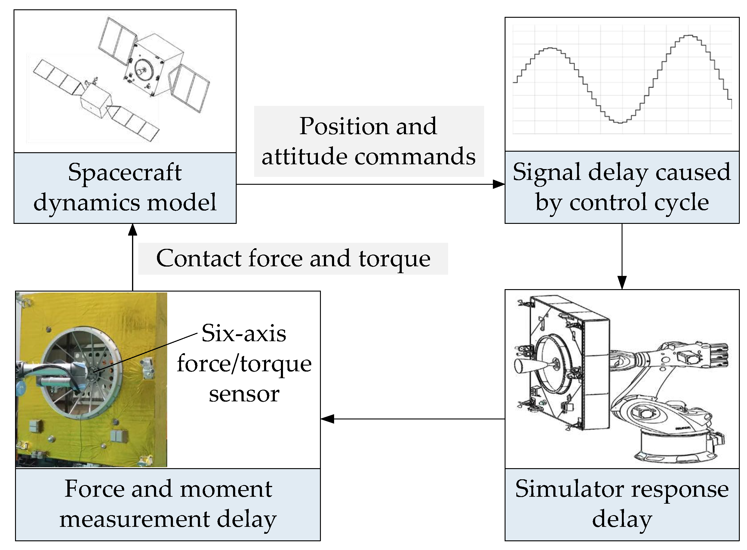
During above process, simulator is affected by factors such as force measurement delay, discrete control cycle, and response delay, resulting in reduced motion accuracy, decreased system stability, and even divergence. To illustrate impact of lagging link on simulator stability and find the corresponding compensation method, considering the complexity of the system, one-dimensional motion of SIT is generally analyzed. The undamped free vibration model is adopted here as shown in Figure 2.
Figure 2.
The 1-DoF undamped free vibration of SIT.
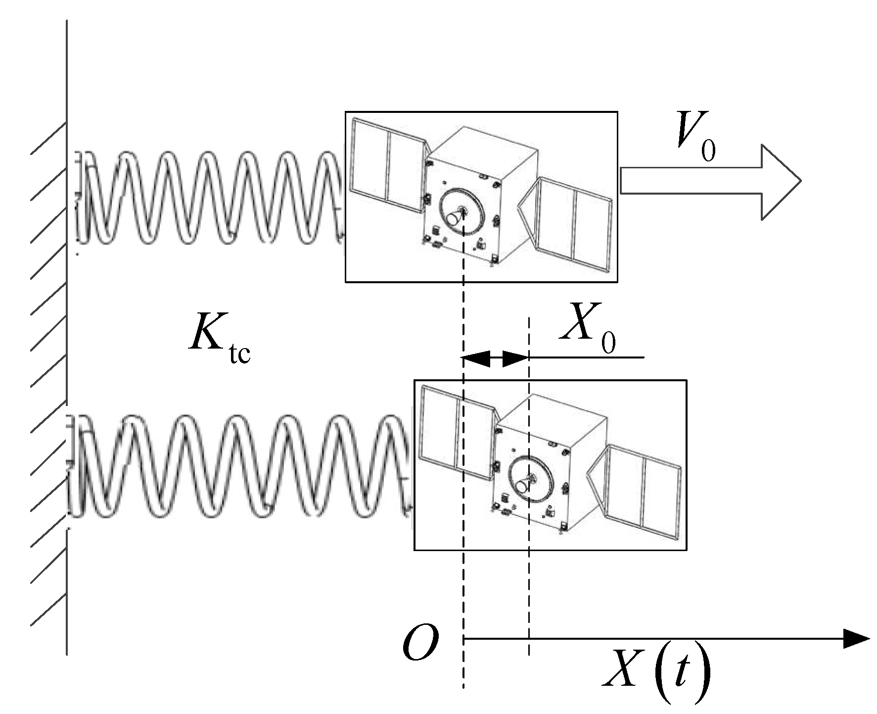
In Figure 2, and are respectively initial velocity and mass of SIT, is the spring stiffness. SIT is theoretically in a free vibration state, and the system is critically stable. The corresponding dynamic equation is given by
where natural frequency is .
2.1. Effect of Force Measurement Delay on System Stability
Let force measurement delay (FMD) be , the vibration differential equation of SIT can be written as
Perform Laplace transform on Equation (2), and the corresponding characteristic equation is
Equation (3) is a transcendental equation, which theoretically has countless characteristic roots. By substituting into the above equation, we can obtain
Separating the real and imaginary parts yields
By solving Equation (5), considering the symmetry of the eigenvalues and only considering solutions with , we can get
Obviously, when , is a pair of conjugate intercepts.
The real component of the derivative of the root locus at all intersection points can be expressed as
A pair of root trajectories enter the right side of the imaginary axis in complex plane when , and they will not return to the left side when . Therefore, the undamped vibration of SIT is unstable for .
To further demonstrate the stability of the time-domain solution in finite time [26], for Equation (2), when , there is
So, Equation (2) is about the stability of in finite time interval. Where and .
In summary, the undamped vibration of SIT with force measurement delay is stable in finite time, but as time approaches infinity, the system gradually diverges.
2.2. Effect of Control Cycle on System Stability
Discrete control cycle keeps the current displacement command for a period of time, which is equivalent to performing a zero order hold on the command signal. The impact model of control cycle can be can be described as follows
Performing the Laplace transform on Equation (9) yields
Undamped vibration model of SIT considering only the effect of control cycle (ECC) is
where is the displacement command considering ECC.
By substituting Equation (10) into the Laplace transform of Equation (11) and performing the inverse Laplace transform, it can be obtained that
To prove its stability, we introduce the following inference.
For equation , where
If has multiple non negative roots, then its corresponding time-delay system is unstable, the equation of which is
We provide proof for the above inference. The corresponding characteristic equation for the third-order time-delay linear system mentioned in Equation (14) is:
On the basis of the stability criterion of the control system, if there are multiple identical zero real part eigenvalues in Equation (15), then its corresponding system is unstable. Let the pure imaginary root be , and by substituting it into Equation (15) and separating the real and imaginary components, we can obtain
Squaring and adding the above equations yields
Let , then Equation (17) can be written as . Due to the presence of multiple non negative roots in f, i.e. also has multiple positive real roots, the delay system is unstable.
Evidently, Equation (12) is one type of Equation (17). Therefore, it can be concluded that when considering control cycle from the above inference, the undamped vibration system with 1-DoF is of divergence.
2.3. Effect of Simulator Response Delay (SRD) on System Stability
Due to the reaction time of electromechanical system, there is a certain delay in the motion response of SITS, and the corresponding differential equation can be written as
where is time-varying delay function.
In terms of the characteristics of the control system, as the motion frequency increases, the phase delay becomes larger, and the response lag reduces the system adaptability to external interference and phase margin. Therefore, 1-DoF undamped movement of SITS is divergent.
3. Mathematical Modeling and Stability Analysis of Hybrid Simulator
3.1. Mathematical Modeling of Hybrid Simulator
To solve the issues of simulation distortion and system divergence, a hybrid simulator is constructed by changing the semi-physical test architecture. The motion signals in the real system are processed and compensated to the dynamic model of one-dimensional undamped vibration of non-cooperative targets, thereby improving the stability of the system. The actual position signal of SITS is processed and compensated into the dynamic model of SIT to improve the stability of the system.
The dynamic equations of the ground semi-physical experimental system, which takes into account FMD, ECC, and SRD before compensation, are as follows
where is the input force of the dynamic model, is equivalent mass, is mass of tracking spacecraft, is displacement command input to SITS considering control cycle, is actual displacement output acquired from SITS controller, and are respectively the orders of SITS dynamic model, and . and are respectively the differential equation coefficients, is the contact damping coefficient.
Overlay the force measurement delay signal with the disposed velocity signal to correct the input of the dynamic model. Let the compensation force be , then rewrite the 6th formula in Equation (19) as follows
where is the gain, which can be a fixed value or a time-varying value.
Perform Laplace transform on Equation (19) and Equation (20), and the corresponding control block diagram of the hybrid simulator is shown in Figure 3.
Figure 3.
Control block diagram of the hybrid simulator.
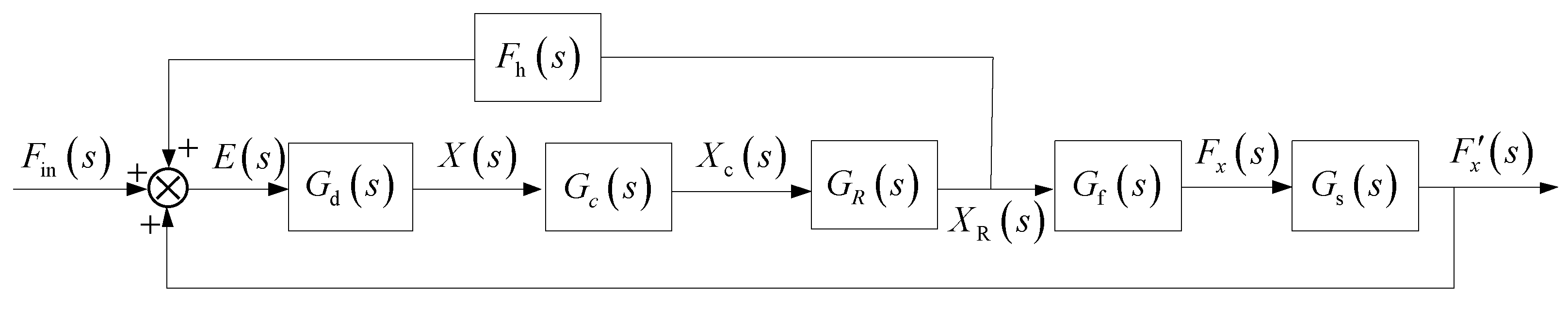
The expressions of and in Figure 3 are
3.2. Model Identification of SITS
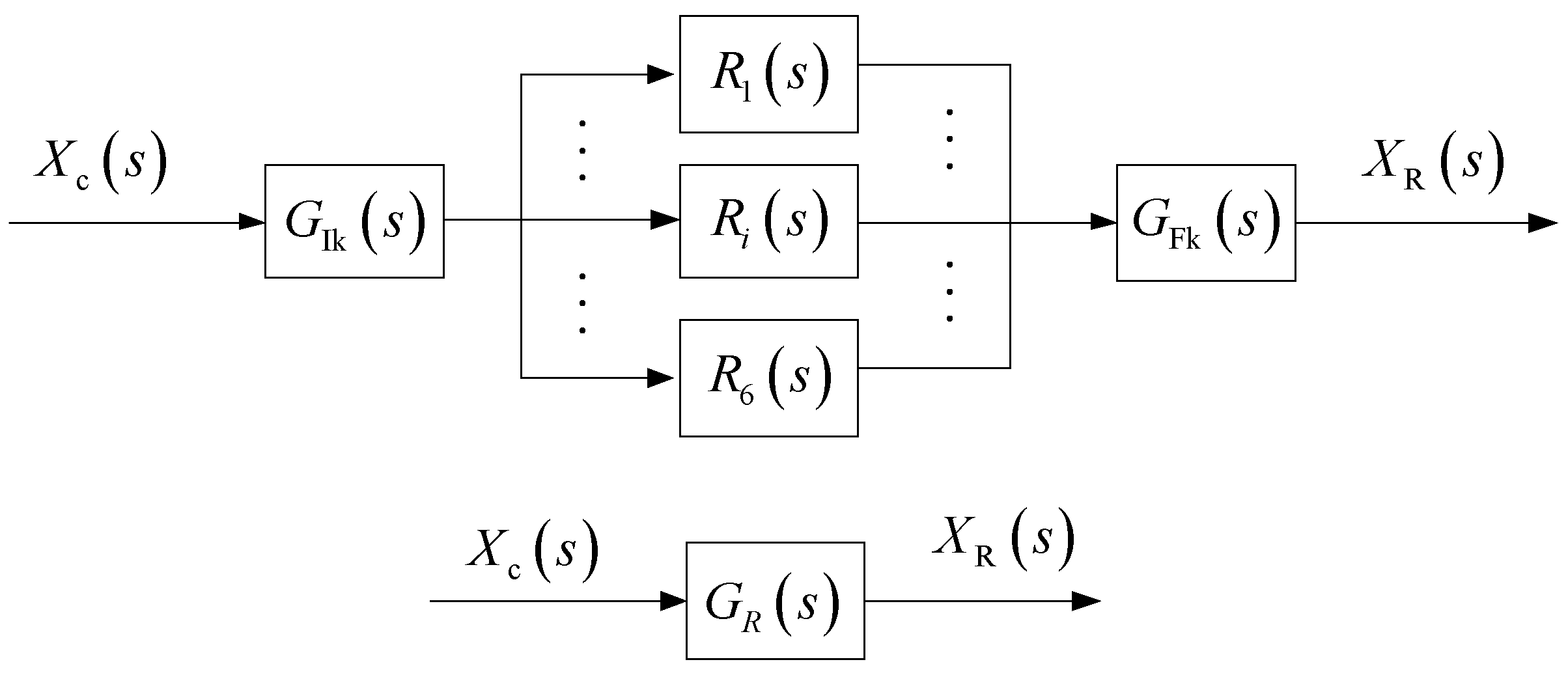
is transfer function of 1D motion of SITS, which mainly includes the forward kinematics model, control model of each joint, and inverse kinematics model, as shown in Figure 4. In practice, is generally obtained through system identification.
Figure 4.
Main constituent models of
In order to comprehensively evaluate the performance of simulator, a certain load is configured, and it is expected that as many axes as possible move simultaneously during the identification. In addition, the motion of simulator should be obvious, making it convenient for real-time measurement by devices such as the laser tracker. Set the 1D motion trajectory as P0→P1→P0→P2→P0→P1→..., as shown in Figure 5.
Figure 5.
The 1D motion trajectory for model identification of SITS.
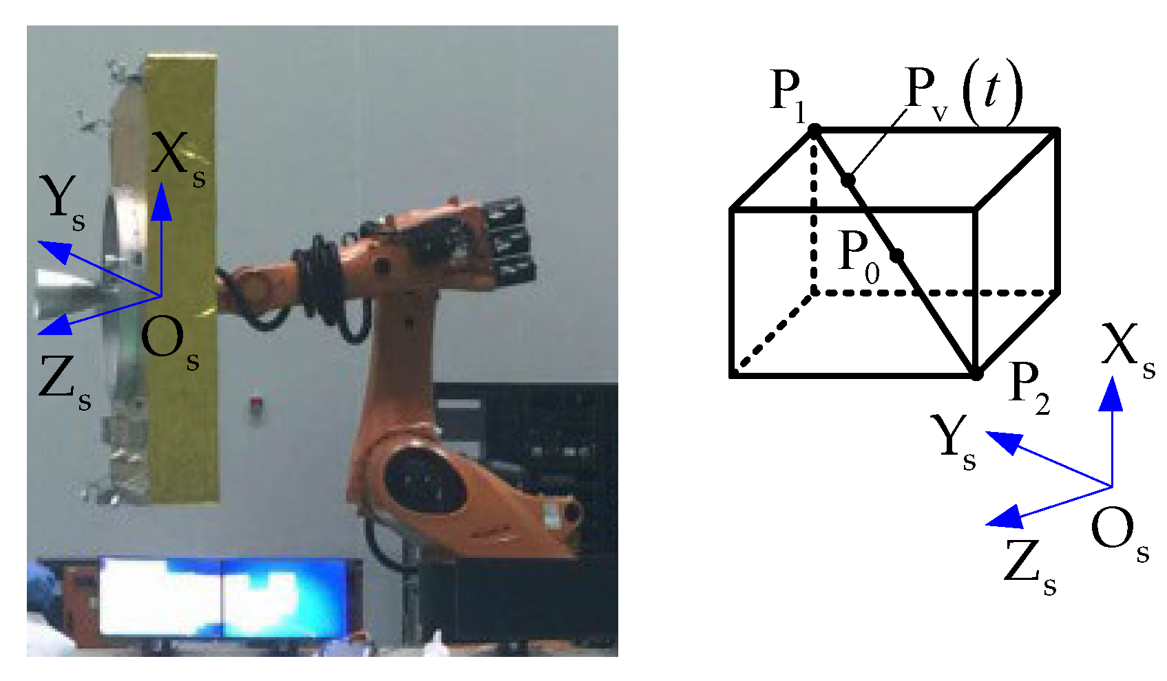
The sweep path equation of the simulator is
where and are amplitude and angular frequency, respectively.
Control point of simulator is located at P0 at initial moment, and the initial velocity is
Let the coordinates of in simulator base coordinate system be , yields
The joint angular displacement corresponding to above Cartesian trajectory can be obtained through robot kinematics model, as follwings
where is the coordinate vector of p0 in the sixth axis coordinate system of SITS, is homogeneous transformation matrix of SITS.
The Z-transform function of SITS can be acquired by applying least squares method to identify the above trajectory in the discrete time domain.
The difference equation corresponding to Equation (27) is
If the number of observed samples is , the least squares estimate of is
where
3.3. Stability and Steady-State Error Analysis
The control block diagram in Figure 3 satisfies
The zero and pole form of identified is given by
where is gain, and are respectively the number of zeros and poles .
Transfer function of SITS can be obtained by performing Laplace transform on the second formula in Equation (20) and substituting it into Equation (31) along with Equation (21), Equation (22) and Equation (32).
The characteristic equation of Equation (33) is given by
From identification results in Section 5, there are two poles and one zero of , so and . Equation (34) is further simplified as
Define the coefficients of system characteristic equations are , then Equation (35) can be rewritten as
where
Owing to good stability and anti-interference ability of industrial robot, and . Considering that and are relatively small, it can be clearly concluded from Equation (37) that , , and .
In terms of Routh stability criterion, Routh array of Equation (36) is given by
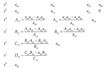
To make sure the stability of SITS, coefficients of the first column of Routh array must be positive, illustrating as in Equation (39).
where
The steady state error of hybrid simulator can be drawn as
When is a step function with the expression as , Equation (41) yields
From the above analysis, it can be concluded that when appropriate parameters are selected, the hybrid simulator proposed is convergent and can achieve stable ground experiments.
4. Delay Compensation Method of Hybrid Simulator
The hybrid simulation model for ground capture experiments of SIT is elaborated above in continuous time domain. Due to the fact that the disposals in physical systems is based on sampled values, the compensation force needs to be discretized. Meanwhile, considering the continuous increase of system energy, an energy observer is introduced to dynamically adjust the gain, and the principle diagram of delay compensation is illustrated in Figure 6.
Figure 6.
Figure 6. Delay compensation principle diagram of hybrid simulator.
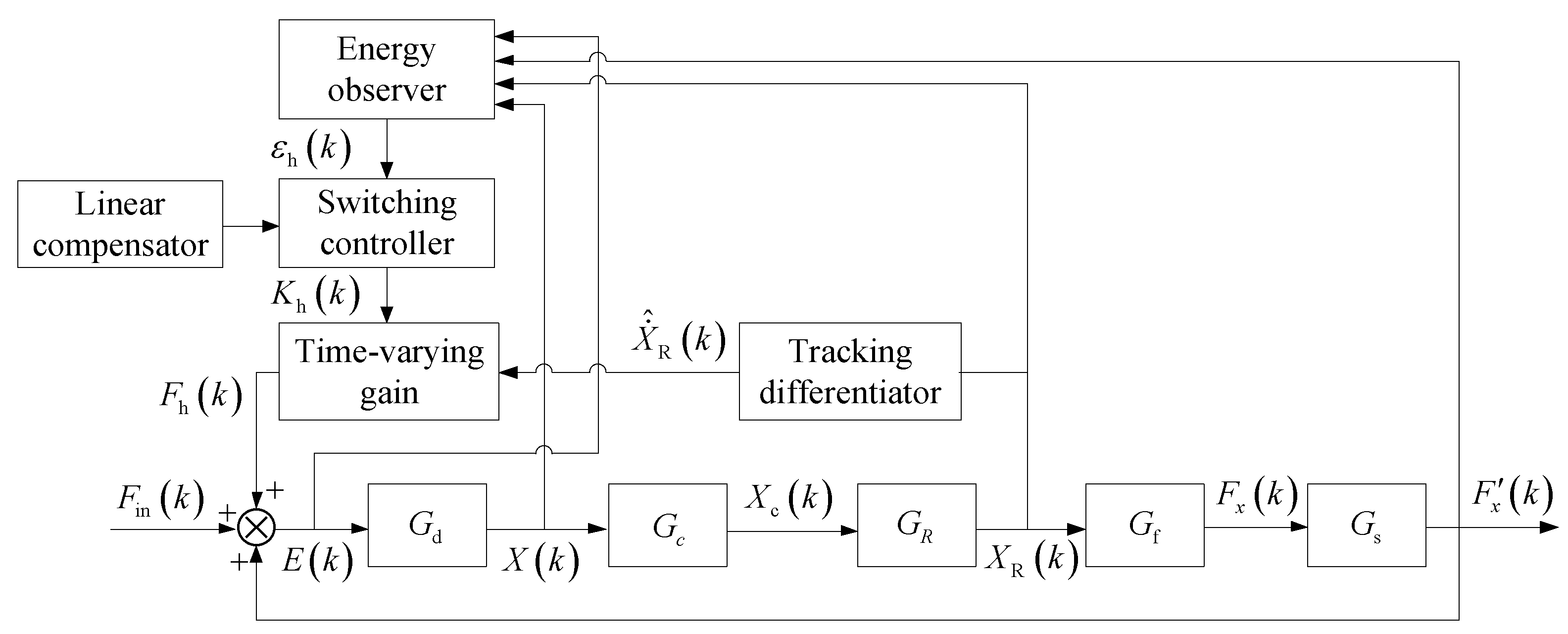
In Figure 6, is the estimation of obtained by tracking differentiator, is the observed energy, is the gain. The k-th force compensation value can be expressed as
where T is system sampling time.
To quantify the performance of proposed compensation method, evaluation indicators of dynamic input force error , SIT velocity error , and recovery coefficient are introduced, the expressions of which are given by
where is the velocity of SIT after compensation, is the absolute value of when takes the maximum value within each vibration cycle.
When the delay compensation method for hybrid simulator achieves good force compensation effect, and should tend towards 0, and should be close to 1.
4.1. Modelling of Switching Compensator with Variable Gain
As time of the ground hybrid simulation system increases, the differences between velocity and recovery force of hybrid simulator and the ideal system become larger without delay compensation, and the system energy will continue to increase. If fixed gain is used for compensation (FGC for short), there will be better tracking performance in the early simulation stage and gradually increasing differences in the later. Although the feedback adjustment ability can vary with time conducting linearized gain for compensation (named as LGC), the effectiveness of this compensation method is also limited when there is a significant nonlinear difference between force and velocity. In terms of the above analysis, a switching compensator with variable gain (SCVG) is constructed, which combines a linearized gain model and a variable gain model based on the energy observer, the latter of which can dynamically adjust with the change of system energy.
reflects the dynamic energy fluctuations during the movement of SITS, which can be drawn as
Because the continuous oscillation of during the movement of SITS, its vibration frequency is twice the natural frequency of SIT. If it is directly introduced into differential negative feedback, it is not conducive to system stability. Therefore, integrating to obtain the feedback gain, the relationship between and is
where is static gain, is variable gain, is switching time.
According to Equation (37), it can be seen that when , varies linearly and also changes continuously with the change of system energy when, which is related to and not entirely dependent on .
When the hybrid simulation system converges, there are
In this circumstances, is finite and is bounded, so there exists that satisfies
For the negative feedback imported by SCVG, is replaced by in Equation (39). In addition, can be acquired through iterative observation, which in turn provides constraints for and , which are also stability constraints for parameters tuning in the discrete domain.
4.2. Velocity Estimation Based on Tracking Differentiator
In the delay compensation approach shown in Fi.6, it is necessary to retrieve the displacement differential signal of hybrid simulator. If the position signal is directly differentiated in discrete time domain, significant noise will be involved and cause distortion of the velocity information, thereby leading to poor compensation performance. Owing to the capacity of optimal tracking differentiator in discrete-time form to rapidly track input signals without overshoot, it has advantages in eliminating signal vibration and improving differentiation quality [33,34,35,36]. Therefore, the discrete optimal tracking differentiator is applied to estimate the SITS velocity.
The actual displacement signal are decomposed into and after passing through the tracking differentiator, where tracks and , thus . The discrete optimal tracking differentiator is given by
where is velocity factor, which determines the tracking speed of . The larger r, the shorter the system step response time, and the faster the command tracking speed. is filtering factor, which suppresses the noise in . is the Optimal control synthesis function, expressed as follows
5. Simulation Study
In order to verify the correctness of the theoretical analysis above and the effectiveness of the proposed delay compensation method, simulation studies are carried out sequentially. Firstly, the comparative analyses are conducted on the SITS stability of 1D undamped vibration under different delays. Then, the response characteristic of SITS identified by the ARX model is demonstrated. Finally, the effectiveness of different delay compensation means on hybrid simulator of ground capture system for SIT is compared. Parameters required for simulation study are shown in Table 1.

Table 1.
The parameters and corresponding values required for numerical simulations.
| Parameter | Value | Unit |
|---|---|---|
| 0.05 | m/s | |
| 500 | Kg | |
| 20000 | N/m | |
| 0.002 | s | |
| 0.004 | s | |
| 50 | N·s/m | |
| 0.025 | m | |
| 6π | rad/s | |
| 0.002 | s | |
| 1501 |
5.1. Simulation Verification of Delays Effect on the SITS Stability of 1D Undamped Vibration
To show the performances of system instability under three different delays FMD, ECC, and SRD, the discrete method is used for solution. The simulation step size for all simulations is set to 0.002s, and the response lag model of simulator adopts the transfer function identified in the next simulation.
The comparisons of velocity , force , and power of SIT under different delay factors are shown in Figure 7. Figure 7(a) shows the comparison of speed and force between idea case and only considering FMD. Figure 7(b) shows the speed and force comparison between FMD and ECC. Figure 7(c) shows the speed and force contrast between idea case and SRD. Figure 7(d) shows the power comparison of SIT under the conditions of no delay and different delays.
Figure 7.
Figure 7. The comparison of velocity, force, and power under different delay factors.

It can be seen from Figure 7 that when there are three different types of delay mentioned above, the 1D undamped system of SIT diverges, but the velocity, force, and power are finite within a specific time interval, which also verifies the analysis and proof of system stability by the aforementioned lags. In the simulation, the delay of FMD has a greater impact than that of ECC, and SRD causes the system to diverge the slowest. Furthermore, the vibration amplitude and energy of SITS under different delay conditions continue to increase compared to the previous cycle. If corresponding compensation is not timely carried out, it will lead to the loss of credibility of ground capture simulation test results, and even damage to the simulator.
5.2. Identification Simulation of SITS
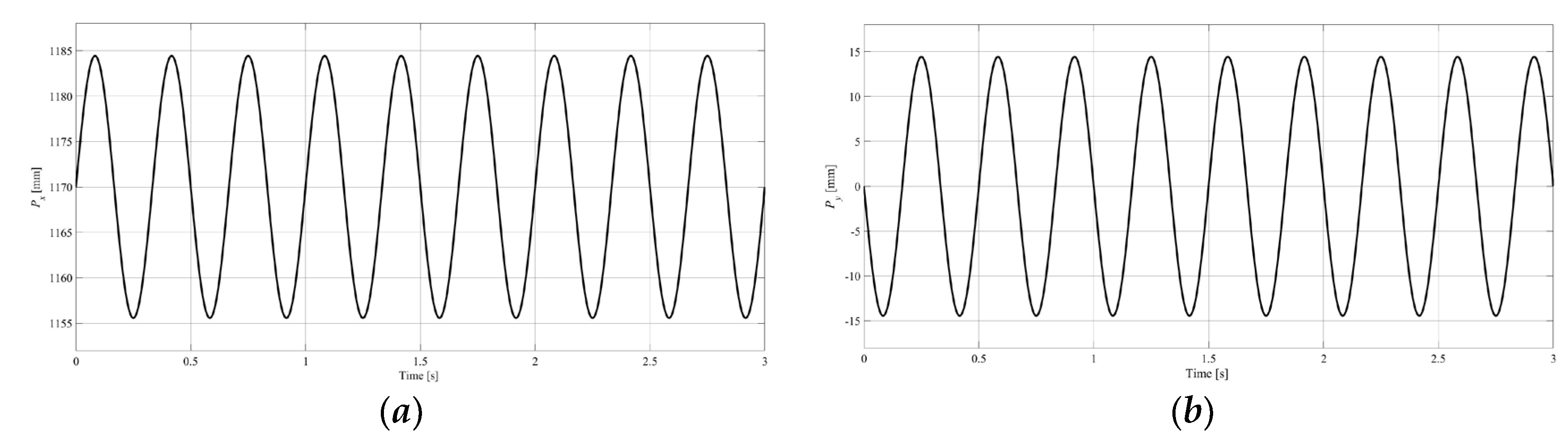
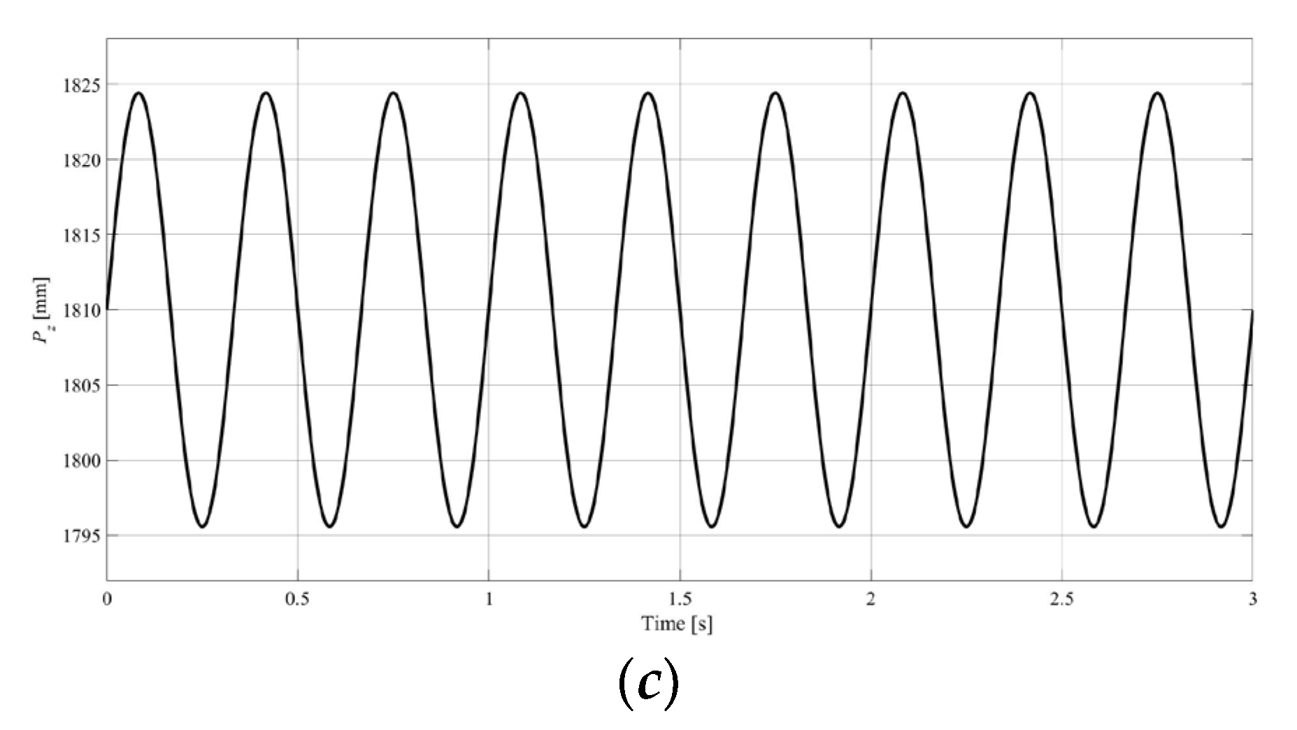
Discretize the sine sweep frequency curves corresponding to the relevant parameters in Table1 and utilize them as control instructions for identifying the discrete domain transfer function of SIST. Then, map the instructions to the Cartesian coordinate system and the joint space of robot through kinematics model. The spatial trajectory of control point Pv is shown in Figure 8.
Figure 8.
The spatial trajectory of Pv.
Taking the above frequency sweep signal as input and the simulated trajectory as output, can be obtained through the mentioned identification algorithm, and can be obtained through transformation. The identified trajectory error is shown in Figure 9(a), and its logarithmic frequency characteristic curve is drawn in Figure 9(b).
Figure 9.
Figure 9. Model identification results of SITS.
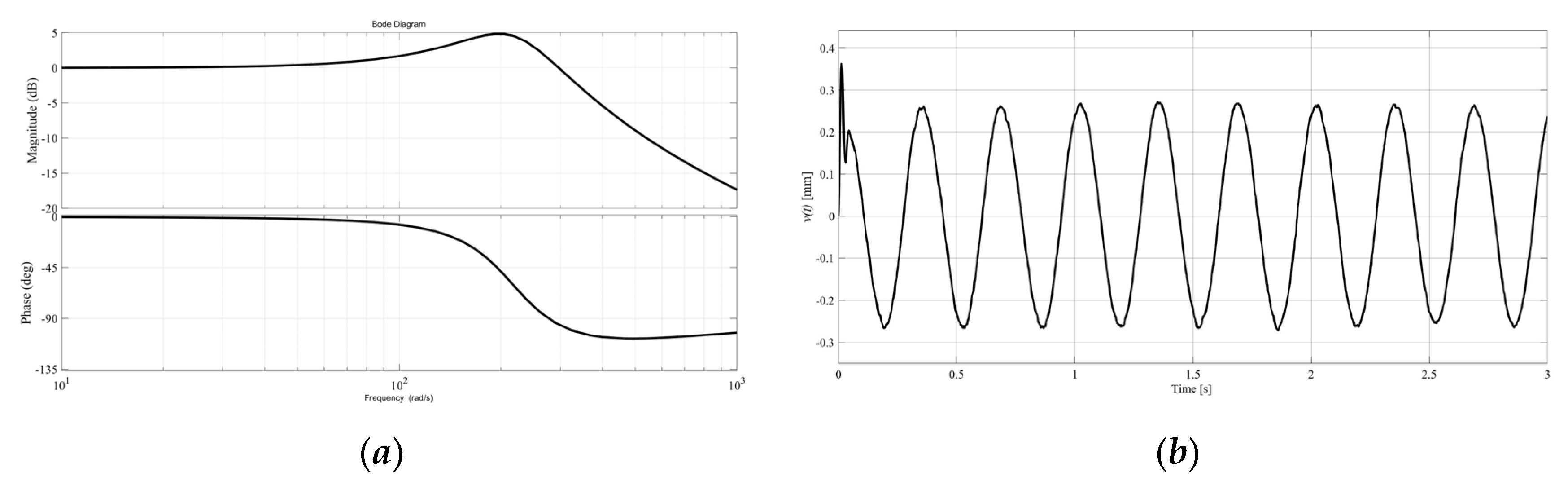
As shown in Figure 9, 1D sweep motion of simulator has a large stability margin. Its amplitude frequency characteristics first increase and then decrease with frequency, while the phase lag continues to increase. At 10Hz, its phase lag is −2.87°.
5.3. Simulation Verification of the Effect for SCVG
To verify the effectiveness of the tracking differentiator and optimize its tuning parameters, Figure 10(a) presents the original displacement curve and direct differential signal of the simulator. Figure 10(b) demonstrates differential signal estimation curves of the original signal corresponding to different tracking differentiator parameters. It can be seen that from Figure 10(a) there are significant spikes and oscillations of the differential signal, and directly applying it for feedback control will reduce system stability. From the partial enlarged view in Figure 10(b), it can be seen that when r is set to a larger value, the estimated tracking speed of its differential signal increases significantly, but its amplitude overshoot also increases. When h takes a larger value, the differential signal becomes stable, but the signal will be distorted due to excessive filtering. Therefore, the parameters of tracking differentiator are selected as after comprehensive consideration, which not only has a fast tracking speed, but also a relatively stable and close to the real differential signal.
Figure 10.
Verification of the tracking differentiator effectiveness. ((a)Original displacement curve and differential signal of the simulator, (b)Differential signal estimations under different tracking differentiator parameters.).
Figure 10.
Verification of the tracking differentiator effectiveness. ((a)Original displacement curve and differential signal of the simulator, (b)Differential signal estimations under different tracking differentiator parameters.).

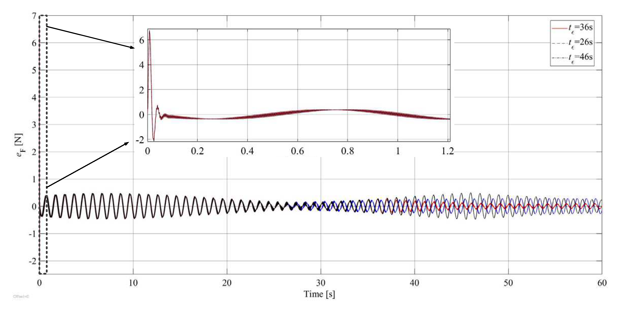
To attain better dynamic compensation effects, plays an critical role to improve the ground experiment accuracy of hybrid simulator in addition to parameter tuning of , and . Fig.11 shows the comparison of when takes different values in SCVG.
From Figure 11, it can be seen that when , the linear compensator takes effect, and the maximum force error after compensation is 6.76N. The nonlinear compensator based on energy observer begins to take effect when , and the peak deviation between the compensated force and the ideal value when is slightly larger than , with a duration of 1s and a maximum deviation of 5.39%. Afterwards, the force error is smaller than and , so it has a better compensation effect when with reducing from 6.76N to 0.09N, which will be used in the following simulations.
Figure 11.
The comparison of when takes different values in SCVG.
To prove the advantage of proposed compensator, the velocity error comparison of SIT under different compensation methods, including FGC, LGC and SCVG, is shown in Figure 12.
Figure 12.
Comparison of SIT velocity error under different compensator.
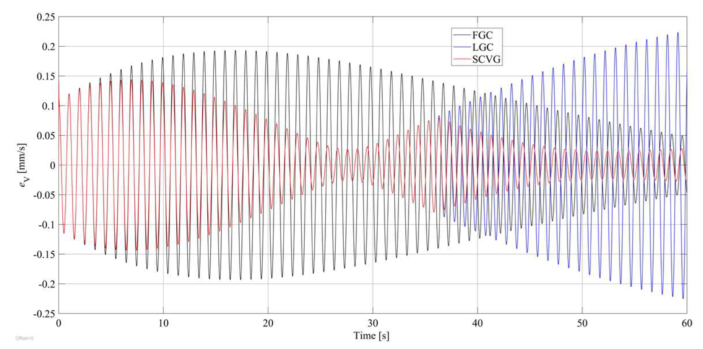
In Figure 12, it can be seen that of LGC is better than that of FGC before the switching control takes effect. The maximum of the former is 0.14mm/s, while the latter is 0.22mm/s. If the nonlinear compensator based on energy observer is not carried out, the velocity error amplitude of LGC exceeds that of FGC at 40.69s. After implementing a nonlinear compensator based on the energy observer, is significantly reduced. At the end of the simulation, the amplitude of is only 0.028mm/s adopting SCVG, while that of LGC and FGC are 0.23mm/s and 0.16mm/s, respectively.
Although is relatively small within the simulation time, due to the continuous attenuation of the vibration velocity, the deviation of its vibration recovery coefficient from the ideal value may become larger. The comparison of the changes of for different compensators is shown in Figure 13.
Figure 13.
The comparison of for different compensators during simulation.
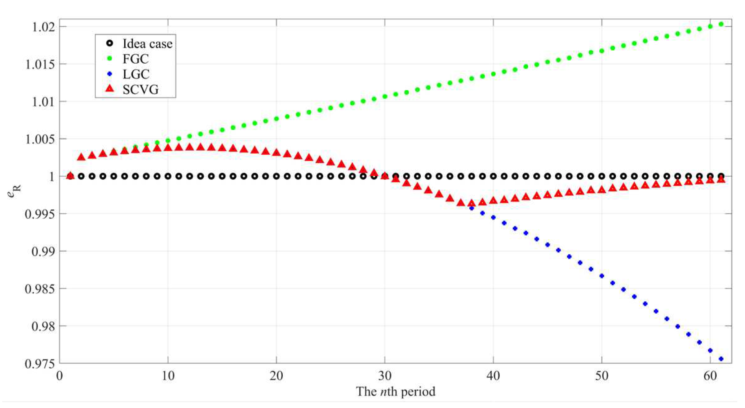
From Figure 13, it can be seen that although of LGC is greater than that of LGC in later stage of simulation, it reduces the energy of the system and thus increases its stability. The of SCVG remains between 0.995 and 1.005, and compared with FGC (1.0203) and LGC (0.9756), it gradually approaches 1 with a value of 0.9995, which also verifies the effectiveness of the proposed compensator.
The movement velocity of SIT is closer to the ideal case without delay due to the adoption of SCVG, which also confirms that the dynamic input force approaches the true value. Figure 14 compares the using different compensators
Figure 14.
Comparison of under different compensators.
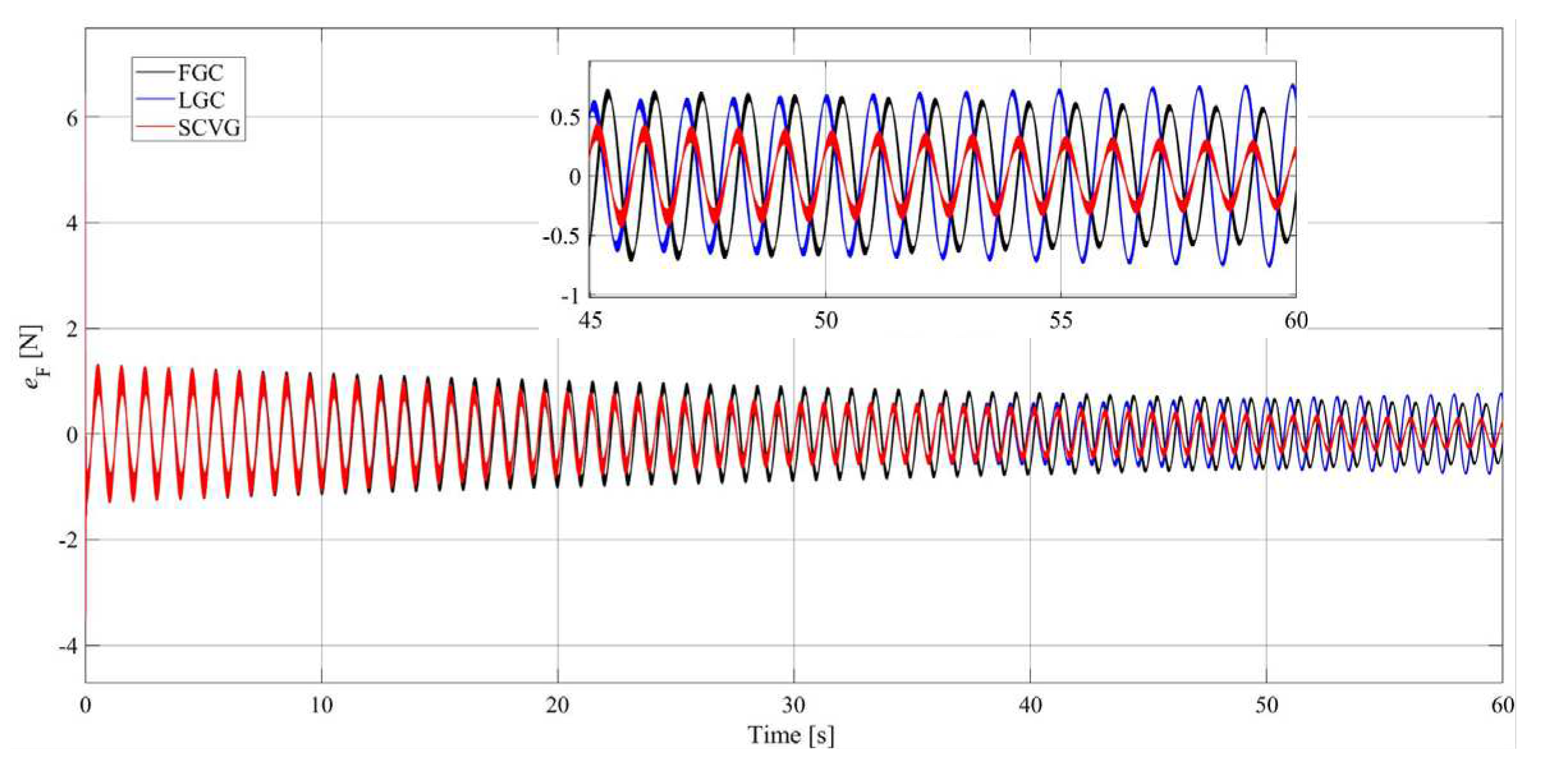
As can be seen from Figure 14, input force errors of three types of compensators are basically the same in initial phase of the simulation, while the differences enlarge gradually as time increases. The value of applying SCVG decreases the fastest, and peak value at the end of simulation is only 0.29N compared with FGC (0.58N) and LGC (0.77N), which verifies the excellent compensation performance of SCVG in long-term hybrid simulation.
The variation of the observed energy of SIT over time adopting SCVG is revealed in Figure 15.
Figure 15.
The variation of adopting SCVG.
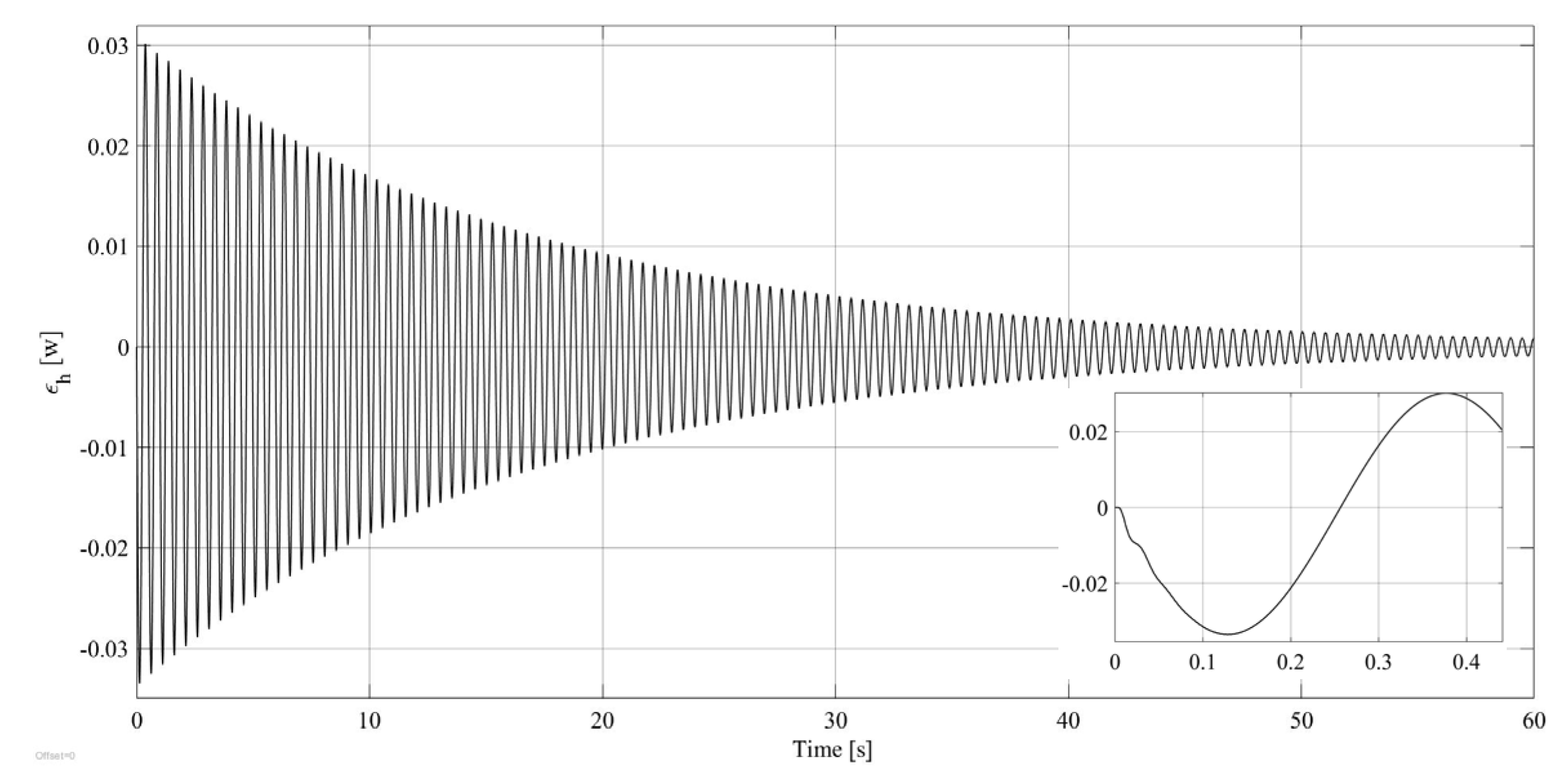
It can be seen from Figure 15 that the value of starts from 0, the amplitude increasing to 0.034w within the first vibration period, and decreases to 8.37×10⁻⁴w in the last simulation cycle, which implies that as the vibration period increases, it eventually tends towards 0, indicating that the system converges. The variation of over time in the proposed SCVG during simulation is shown in Figure 16.
Figure 16.
The variation of in SCVG during simulation.
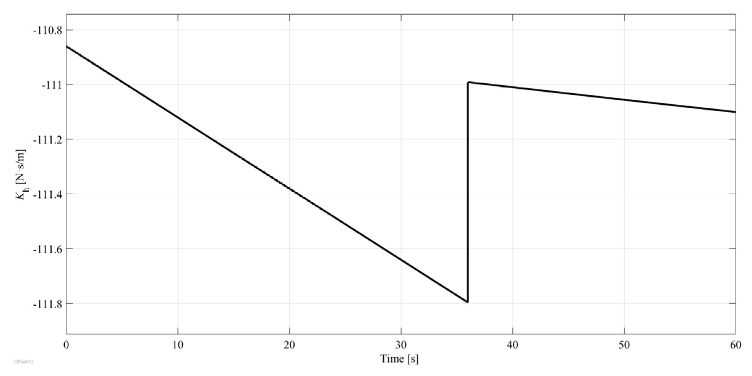
Feedback compensation gain varies linearly with time before the switching controller taking effect. As system energy gradually stabilizes in the later phase of simulation, it actually exhibits nonlinear changes, which means that SITS is corrected in a timely manner after the switch time.
Furthermore, the values of and can also be acquired, which are and , respectively. The SITS system has two characteristic roots with positive real parts when , and the system is unstable. It can be concluded that the eigenvalues all have negative real parts by substituting and into characteristic Equation (36) and it simultaneously satisfies the stability constraints of Equation (39), indicating that the SITS is asymptotically stable. Therefore, the proposed hybrid simulation system with SCVG is stable.
6. Conclusions
(1) A hybrid simulator is proposed based on SCVG after analyzing the instability of simulator in current SPS systems caused by three types of delays. The stability constraints of the proposed hybrid simulator are obtained adopting the Routh criterion, and the simulation study is employed to verify the effectiveness and stability of the proposed compensation method.
(2) The proposed SCVG consists of variable gain and velocity estimator, which modifies input force of dynamic model through switching control. Velocity estimation is achieved by approximating tracking of differential signal of the actual displacement applying the optimal tracking differentiator. The nonlinear gain model automatically adjusts the feedback gain according to the current observed energy variation of the system.
(3) The peak errors of dynamic input, velocity, and recovery coefficient adopting SCVG in the last cycle before the end of simulation are 0.29N, 0.028mm/s, and 0.0005, respectively. Compared with FGC and LGC, the performance improvements are at least 50.00%, 82.50%, and 97.54%.
(4) The proposed SCVG demonstrates excellent compensation effects for the 1D motion of the hybrid simulator in simulation of ground capture test systems. In future work, we aim to extend the proposed compensator to 6-DoF spatial motion, further enhancing the stability of the hybrid simulator. The future research is to develop a universal hybrid simulator with high-fidelity in the ground capture mission trials.
Author Contributions
Author Contributions: Conceptualization, X.B. and Z.X.; methodology, X.B. and X.L.; software, X.B. and M.L.; validation, H.L. and Z.Z.; writing—review and editing, X.B. and H.L.; supervision, X.L.; project administration, Z.Z. and Z.X. All authors have read and agreed to the published ver-sion of the manuscript.
Funding
This research was supported by the space debris mitigation research project (KJSP2020010303) funded by State Administration of Science, Technology and Industry for National Defence, PRC.
Data Availability Statement
Data are contained within the article.
Conflicts of Interest
The authors declare no conflicts of interest.
References
- Keles O F. Telecommunications and Space Debris: Adaptive Regulation Beyond Earth. Telecommun Policy 2023, 47, 102517. [CrossRef]
- Takeichi, N.; Tachibana, N. A tethered plate satellite as a sweeper of small space debris. Acta Astronaut 2021, 189, 429–436. [CrossRef]
- Witze, A. The quest to conquer earth's space junk problem. Nature 2018, 561, 24–26. [CrossRef]
- A. Nanjangud, P.C. Blacker, S. Bandyopadhyay, Y. Gao. Robotics and AI-Enabled On-Orbit Operations With Future Generation of Small Satellites. P Ieee 2018, 106, 429-439. [CrossRef]
- N. Inaba, M. Oda, M. Asano. Rescuing a Stranded Satellite in Space-Experimental Robotic Capture of Non-Cooperative Satellites. T Jpn Soc Aeronaut S 2006, 48, 213-220. [CrossRef]
- E. Papadopoulos, F. Aghili, O. Ma, R. Lampariello. Robotic Manipulation and Capture in Space: A Survey. Front Robot Ai 2021, 8, 686723. [CrossRef]
- T. Rybus. Obstacle avoidance in space robotics: Review of major challenges and proposed solutions. Prog Aerosp Sci 2018, 101, 31-48. [CrossRef]
- H. G. Hatch, J. E. Pennington, and J. B. Cobb. Dynamic simulation of lunar module docking with Apollo command module in lunar orbit. NASA Tech. Note TN D-3972, 1967, pp. 1–26.
- Uyama N, Fujii Y, Nagaoka K, et al. Experimental evaluation of contact-impact dynamics between a space robot with a compliant wrist and a free-flying object. International symposium on artificial intelligence, robotics and automation in space, Turin, Italy. 2012.
- Wei, Y., Yang, X., Xu, Z., Bai, X. Novel ground microgravity experiment system for a spacecraft-manipulator system based on suspension and air-bearing. Aerosp Sci Technol 2023, 141, 108587. [CrossRef]
- O. Ma and J. Wang. Model order reduction for impact-contact dynamics simulations of flexible manipulators. Robotica 2007, 25, 397–407. [CrossRef]
- A. Flores-Abad, O. Ma, K. Pham, S. Ulrich. A review of space robotics technologies for on-orbit servicing. Prog Aerosp Sci 2014, 68, 1–26. [CrossRef]
- A. Yaskevich. Real time math simulation of contact interaction during spacecraft docking and berthing. J. Mech. Eng. Autom 2014, 4, 1–15.
- Roe F D, Howard R T, Murphy L. Automated rendezvous and capture system development and simulation for NASA. Modeling, Simulation, and Calibration of Space-based Systems. SPIE 2004, 5420: 118-125.
- Mitchell, J. D., Cryan, S. P., Baker, K., Martin, T., Goode, R., Key, K. W., Chien, C. H. Integrated docking simulation and testing with the Johnson space center six-degree-of-freedom dynamic test system. In Proc. Space Technol. Appl. Int. Forum, 2008, pp. 709–716.
- Boge T , Ma O .Using advanced industrial robotics for spacecraft Rendezvous and Docking simulation. In 2011 IEEE international conference on robotics and automation, pp. 1-4.
- O. Ma, A. Flores-Abad, and T. Boge. Use of industrial robots for hardware-in-the-loop simulation of satellite rendezvous and docking. Acta Astronaut 2012, 81, 335–347. [CrossRef]
- Wei YQ, Yang X, Bai XL, Xu ZG. Hardware-in-the-loop based ground test system for space berthing and docking mechanism of small spacecraft. P I Mech Eng G-J Aer 2023, 237, 3486-3495. [CrossRef]
- Zebenay, M., Lampariello, R., Boge, T., Choukroun, D. A new contact dynamics model tool for hardware-in-the-loop docking simulation. 2012.
- Zebenay M, Boge T, Krenn R, et al. Analytical and experimental stability investigation of a hardware-in-the-loop satellite docking simulator. P I Mech Eng G-J Aer 2015, 229, 666-681. [CrossRef]
- Qi, C., Ren, A., Gao, F., Zhao, X., Wang, Q., Sun, Q. Compensation of velocity divergence caused by dynamic response for hardware-in-the-loop docking simulator. Ieee-Asme T Mech 2016, 22, 422-432. [CrossRef]
- Stefano M D, Balachandran R, Secchi C. A Passivity-Based Approach for Simulating Satellite Dynamics With Robots: Discrete-Time Integration and Time-Delay Compensation. Ieee T Robot 2020, 36, 189-203. [CrossRef]
- Rao, L. S., Rao, P. S., Chhabra, I. M., Kumar, L. S. Modeling and Compensation of Time-Delay Effects in HILS of Aerospace Systems. Iete Tech Rev 2022, 39, 375-388. [CrossRef]
- Osaki K, Konno A, Uchiyama M. Delay time compensation for a hybrid simulator. Adv Robotics 2010, 24, 1081-1098. [CrossRef]
- Abiko, S., Satake, Y., Jiang, X., Tsujita, T., Uchiyama, M. Delay time compensation based on coefficient of restitution for collision hybrid motion simulator. Adv Robotics 2014, 28, 1177-1188. [CrossRef]
- Khusainov, D. Y., Diblík, J., Růžičková, M., Lukáčová, J. Representation of a solution of the Cauchy problem for an oscillating system with pure delay. Nonlinear Oscil 2008, 11, 276-285. [CrossRef]
- Ricardo L G G, Lagomasino G L. Strong asymptotics of multi-level Hermite-Padé polynomials. J Math Anal Appl 2024, 531, 127801. [CrossRef]
- Đukić, D., Mutavdžić Đukić, R., Reichel, L., Spalević, M. Optimal averaged Padé-type approximants. Electron T Numer Ana 2023, 59, 145-156. [CrossRef]
- Motoyama Y, Yoshimi K, Otsuki J. Robust analytic continuation combining the advantages of the sparse modeling approach and the Padé approximation. Phys Rev B 2022, 105, 035139. [CrossRef]
- Mehmood, K., Chaudhary, N. I., Cheema, K. M., Khan, Z. A., Raja, M. A. Z., Milyani, A. H., Alsulami, A. Design of nonlinear marine predator heuristics for hammerstein autoregressive exogenous system identification with key-term separation. Mathematics 2023, 11, 2512. [CrossRef]
- Beltran-Perez, C., Serrano, A. A., Solís-Rosas, G., Martínez-Jiménez, A., Orozco-Cruz, R., Espinoza-Vázquez, A., Miralrio, A. A general use QSAR-ARX model to predict the corrosion inhibition efficiency of drugs in terms of quantum mechanical descriptors and experimental comparison for lidocaine. Int J Mol Sci 2022, 23, 5086. [CrossRef]
- Mehmood, K., Chaudhary, N. I., Khan, Z. A., Cheema, K. M., Raja, M. A. Z., Shu, C. M. Novel knacks of chaotic maps with Archimedes optimization paradigm for nonlinear ARX model identification with key term separation. Chaos Soliton Fract 2023, 175, 114028. [CrossRef]
- Wen, Q., Wang, M., Li, X., Chang, Y. Learning-based design optimization of second-order tracking differentiator with application to missile guidance law. Aerosp Sci Technol 2023, 137, 108302. [CrossRef]
- Park J H, Park T S, Kim S H. Asymptotically convergent higher-order switching differentiator. Mathematics 2020, 8, 185. [CrossRef]
- Feng H, Qian Y. A linear differentiator based on the extended dynamics approach. Ieee T Automat Contr 2022, 67, 6962-6967. [CrossRef]
- Oliveira T R, Estrada A, Fridman L M. Global and exact HOSM differentiator with dynamic gains for output-feedback sliding mode control. Automatica 2017, 81, 156-163. [CrossRef]
Disclaimer/Publisher’s Note: The statements, opinions and data contained in all publications are solely those of the individual author(s) and contributor(s) and not of MDPI and/or the editor(s). MDPI and/or the editor(s) disclaim responsibility for any injury to people or property resulting from any ideas, methods, instructions or products referred to in the content. |
© 2024 by the authors. Licensee MDPI, Basel, Switzerland. This article is an open access article distributed under the terms and conditions of the Creative Commons Attribution (CC BY) license (http://creativecommons.org/licenses/by/4.0/).
Copyright: This open access article is published under a Creative Commons CC BY 4.0 license, which permit the free download, distribution, and reuse, provided that the author and preprint are cited in any reuse.


