Preprint

Article

Evolutionary Reinforcement Learning of Neural Network Controller for Acrobot Task — Part3: Differential Evolution

Altmetrics

Downloads

Views

Comments

Hidehiko Okada^*

This version is not peer-reviewed

Submitted:

01 February 2024

Posted:

02 February 2024

You are already at the latest version

Alerts

Abstract

Evolutionary algorithms find applicability in reinforcement learning of neural networks due to their independence from gradient-based methods. To achieve successful training of neural networks using evolutionary algorithms, careful considerations must be made to select appropriate algorithms due to the availability of various algorithmic variations. In Part1 and Part2, the author previously reported experimental evaluations on Genetic Algorithm and Evolution Strategy for reinforcement learning of neural networks, utilizing the Acrobot control task. This article constitutes Part3 of the series of comparative research. In this study, Differential Evolution is adopted as the third instance of major evolutionary algorithms. The experimental results show a statistically significant superiority of DE over both GA and ES (p < .01). In addition, DE exhibits its robustness to variations in hyperparameter configurations (the number of offsprings and generations). In the previous experiments, both ES and GA showed significant performance differences depending on the configurations, whereas in the experiment reported in this article, such differences are not detected for DE.

Keywords:

Subject: Computer Science and Mathematics - Artificial Intelligence and Machine Learning

1. INTRODUCTION

Neural networks can be effectively trained using gradient-based methods for supervised learning tasks, where labeled training data are available. However, when it comes to reinforcement learning tasks where labeled training data are not provided, neural networks demand the utilization of gradient-free training algorithms. Evolutionary algorithms [1,2,3,4,5] find applicability in the reinforcement learning of neural networks due to their independence from gradient-based methods.

Evolution Strategy [6,7], Genetic Algorithm [8,9,10,11], and Differential Evolution [12,13,14] stand as representative evolutionary algorithms. To achieve successful training of neural networks using evolutionary algorithms, careful considerations must be made regarding: i) selecting appropriate algorithms due to the availability of various algorithmic variations, and ii) designing hyperparameters as they significantly impact performance. The author previously reported experimental evaluations on Genetic Algorithm and Evolution Strategy for reinforcement learning of neural networks, utilizing the Acrobot task [15,16]. In this study, Differential Evolution is adopted as another instance of major evolutionary algorithms.

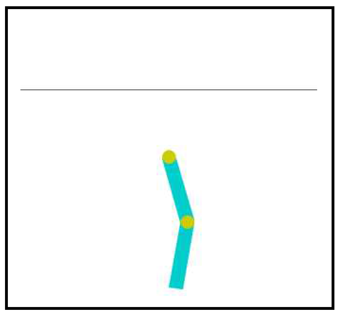
2. ACROBOT CONTROL TASK

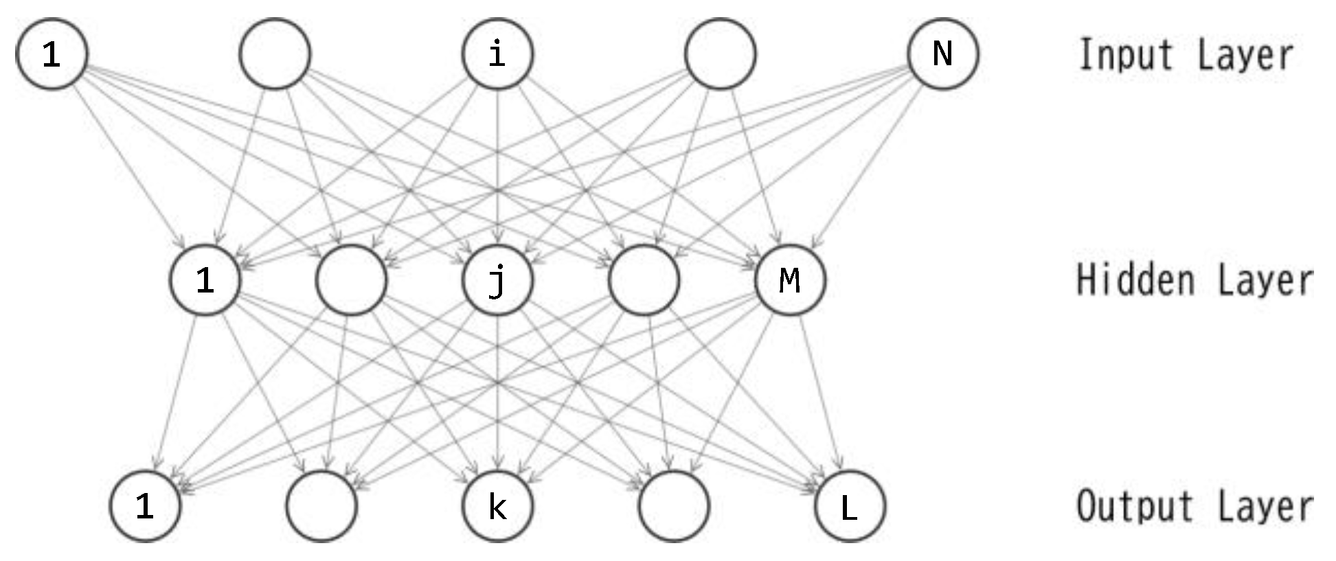
As a task that requires reinforcement learning to solve, this study employs Acrobot control task provided at OpenAI Gym. Figure 1 shows a screenshot of the system. This task is the same as that in the previous study; details on this task were described in Part1 [16]. The same method for scoring fitness of a neural network controller (eq.(1) in Part1) is employed again in this study.

3. NEURAL NETWORKS

In the previous studies using GA and ES [15,16], the author employed a three-layered feedforward neural network known as a multilayer perceptron (MLP [17,18]) as the controller. The same MLP is utilized again in this study. Figure 2 illustrates the topology of the MLP. The feedforward calculations were described in Part1 [16]. In all of this study and the previous ones, the MLP serves as the policy function: action(t) = F(observation(t)). The input layer consists of six units, each corresponding to the values obtained by an observation. To ensure the input value falls within the range [-1.0, 1.0], the angular velocity of θ₁ (θ₂) is divided by

4 π

(

9 π

). The output layer comprises one unit, and its output value is applied as the torque to the joint.

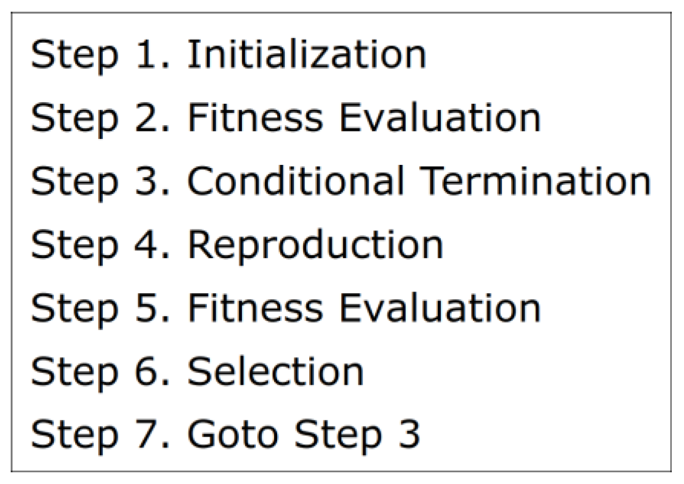
4. TRAINING OF NEURAL NETWORKS BY DIFFERENTIAL EVOLUTION

The three-layered perceptron depicted in Figure 2 includes M+L unit biases and NM+ML connection weights, resulting in a total of M+L+NM+ML parameters. Let D represent the quantity M+L+NM+ML. For this study, the author sets N=6 and L=1, leading to D=8M+1. The training of this perceptron is essentially an optimization of the D-dimensional real vector. Let

x = (x_{1}, x_{2}, . . ., x_{D})

denote the D-dimensional vector, where each

x_{i}

corresponds to one of the D parameters in the perceptron. By applying the value of each element in

x

to its corresponding connection weight or unit bias, the feedforward calculation (described by eqs. (2)-(6) in Part1 [16]) can be processed.

In this study, the D-dimensional vector

x

is optimized using Differential Evolution [12,13,14]. DE treats

x

as a chromosome (a genotype vector) and applies evolutionary operators to manipulate it. The fitness of

x

is evaluated based on eq. (1) described in Part1 [16]. Figure 3 illustrates the DE process. Steps 1-3 are the same as those in Evolution Strategy, which are described in Part1 [16]. Step 1 initializes vectors

y^{1}

y^{2}

, …,

y^{λ}

randomly within a predefined range, denoted as

{[m i n, m a x]}^{D}

, where

λ

represents the number of offsprings. In Step 2, the values in each vector

y^{c}

(c=1, 2, ...,

λ

) are fed into the MLP, which subsequently controls the Acrobot system for a single episode consisting of 200 time steps. The fitness of

y^{c}

is evaluated based on the outcome of the episode. In Step 3, the evolutionary training loop concludes upon meeting a preset condition. A straightforward example of such a condition is reaching the limit number of fitness evaluations.

In Step4, new

λ

offsprings are created by applying the crossover operator to the parents

y^{1}

y^{2}

, …,

y^{λ}

and donors. The donors are created before the crossover. The reproduction scheme called DE/rand/1/bin is adopted in this study. Let

v^{c}

denote a genotype vector of the c-th donor;

v^{c} = {(v}_{1}^{c}, v_{2}^{c}, \dots, v_{D}^{c}),

c=1, 2, ...,

λ

v^{c}

is determined as follows:

Among the parents $y^{1}, y^{2}, \dots, y^{λ}$ , three parents $y^{i}, y^{j}, y^{k}$ are randomly selected where $i \neq j \neq k \neq c$ .
$v_{d}^{c} = y_{d}^{i} + F (y_{d}^{j} - y_{d}^{k}),$ d=1, 2, …, D, where $F$ is a preset scaling factor.

Let

z^{c}

denote a genotype vector of the c-th offspring;

z^{c} = {(z}_{1}^{c}, z_{2}^{c}, \dots, z_{D}^{c}),

c=1, 2, ...,

λ

z^{c}

is determined as follows:

z_{d}^{c} = \{\begin{array}{l} v_{d}^{c}, rand < CR or d = RAND, \\ y_{d}^{c}, else . \end{array}

(1)

In eq.(1), c=1, 2, ...,

λ

and d=1, 2, …, D. CR is a preset crossover rate, 0

\leq

\leq

1. RAND is a uniform random integer, RAND

\in

{1, 2, …, D}. RAND and rand are sampled for each c

\in

{1, 2, ...,

λ

}. Any element of the new offspring vectors is truncated to the domain [

m i n, m a x

] if the element exceeds the domain. In Step5, fitness of each offspring

z^{c}

is evaluated by the same method as each parent

y^{c}

is. In Step6, the better of the parent

y^{c}

or the offspring

z^{c}

is selected as a new parent

y^{c}

(c=1, 2, ...,

λ

) for the next generation.

5. EXPERIMENT

In the previous studies using GA and ES, the number of fitness evaluations included in one experiment trial was set to 5,000 [15,16]. The number of new offsprings generated per generation,

λ

, was either of (a) 10 and (b) 50. The number of generations was 500 for (a) and 100 for (b) respectively. The total number of fitness evaluations were 10 × 500 = 5,000 for (a) and 50 × 100 = 5,000 for (b). The experiment using DE in this study employed the same settings. The hyperparameter configurations for DE are shown in Table 1.

The domain of genotype vectors,

{[m i n, m a x]}^{D}

, was kept consistent with the previous experiments [15,16], i.e., [-10.0, 10.0]^D. The number of hidden units, M, was also consistently set to the four variations: 4, 8, 16, and 32. An MLP with either of 4, 8, 16, or 32 hidden units underwent independent training 11 times. Table 2 presents the best, worst, average, and median fitness scores of the trained MLPs across the 11 trials. Each of the two hyperparameter configurations (a) and (b) in Table 1 was applied.

Comparing the scores in Table 2 between configurations (a) and (b), there is no clear commonality in the relationship between the two configurations, i.e. scores of (a) is sometimes larger and vice versa. The Wilcoxon signed rank test confirmed that the difference between scores of configuration (a) and those of (b) was not statistically significant (p = .35), while configuration (a) was slightly better. In previous studies, configuration (b) contributed significantly better for ES [16], while configuration (a) contributed significantly better for GA [15]. Configuration (a) promotes exploitation in the later stage of search due to the large number of generations, and configuration (b) promotes exploration in the early stage of search due to the large number of offsprings. Since ES is not good at exploration, configuration (b) compensates for this disadvantage. On the other hand, since GA is not good at exploitation, configuration (a) compensates for this disadvantage. There was no significant difference between the two configurations for DE, indicating that DE performed a better balance between exploration and exploitation than ES and GA did.

Next, upon comparing the fitness scores obtained using configuration (a) among the four variations of M (the number of hidden units), it is observed that the scores with M=4 are worse than those of M=8, 16 and M=32. The Wilcoxon rank sum test confirmed that the difference between M=4 and either of M=8, 16, or 32 was statistically significant (p = .044, .033 and .058 respectively). No other difference was found to be statistically significant. This result indicates that 4 hidden units are not sufficient for this task, which is consistent with the previous study [15]. Although the difference between M=8 and either of M=16 or 32 was not statistically significant, the p-values obtained by the test showed that M=8 was better than both of M=16 and M=32. It can be concluded that, in this task, M=8 was the best choice in terms of performance and model size, which is also consistent with the previous study [15,16].

Figure 4 presents learning curves of the best, median, and worst runs among the 11 trials where the configuration is (a). Note that the horizontal axis of these graphs is in a logarithmic scale. The shapes of these graphs are similar to the results of the previous experiments using GA and ES [15,16], and the manner in which the fitness scores became larger along with the progression of evaluation counts showed a common pattern among the three algorithms. In these graphs, the fitness scores started at nearly 0.0 and eventually rose to around 0.4 to 0.45, but in the meantime, there were two intervals in which the increase in the scores stagnated and the graph became roughly flat. The first flat interval appeared from the first to the tenth evaluations, and the fitness scores were less than 0.1. The second flat interval occurred from the 10th to the 100th evaluations where the scores were 0.2 to 0.3. The first flat interval occurred because it took time to learn to swing the Acrobot chains. The second flat interval occurred because it took time again to learn from the time the chains began to rotate (so that the free end of linear chains exhibited periodic oscillations between ascent and descent) until it became possible to maintain the free end at higher positions. For all the four M variations, even in the worst trials the final fitness scores are not significantly worse than the corresponding best trials. This indicates that DE could robustly optimize the MLP so that the variance was small within the 11 trials.

Figure 5(a) illustrates the actions by the MLP and the heights p_y(t) (see eq. (1) in Part1 [16]) in the 200 steps prior to training, while Figure 5(b) displays the corresponding actions and heights after training. Supplementary videos are provided which demonstrate the motions of the chain2^,3. In this scenario, the MLP employed 8 hidden units, and the configuration (a) in Table 1 was utilized. In the previous articles [15,16] which reported the corresponding results by GA and ES, the action and the heights are illustrated in Figure 5(a)(b). The three Figure 5(a) appear to be similar: before training, the MLPs could only output values close to -1 during the 200 steps and the Acrobot chain hardly moved, resulting in the heights p_y(t) hardly increasing from the initial 0.0. On the other hand, when comparing Figure 5(b) among DE, GA, and ES, the figure for DE (Figure 5(b) in this article) is particularly similar to the corresponding figure for GA (Figure 5(b) in [15]). From the 1st step to around 75 steps, the action values alternated approximately between -1 and 1. As a result, the Acrobot chain swung and the heights rose to approximately 0.8. Afterwards, until the last step, the heights were generally maintained at 0.5 or above, and when the heights fell below 0.5, they were quickly risen back to above 0.5.

Compared to Figure 5(b) in [16] for ES, Figure 5(b) in this article for DE and Figure 5(b) in [15] for GA showed smaller number of times where the heights fell below 0.5 in the later steps. This means that DE and GA could train the MLPs more appropriately than ES so that the trained MLPs became able to adjust the torque to keep the free end of the Acrobot chain at a height of 0.5 or more. However, even in the case of DE, it was not possible for the trained MLP to maintain the entire chain in an inverted state and bring the free end of the chain to the highest position at 1.0, which was the same as the result with GA and ES.

6. STATISTICAL TEST TO COMPARE DE WITH GA AND ES

The author conducted a Wilcoxon signed rank test to investigate whether there was a statistically significant difference between the fitness scores obtained from the previous experiments using GA [15] or ES [16] and those from the experiment using DE in this study. The data used for this test included the 32 values reported in Table 2 of Part1 [16] (the data obtained using ES), those in Table 2 of Part2 [15] (the data obtained using GA), and those in Table 2 of this article (the data obtained using DE). The test result indicated that DE was significantly superior to both of GA (p < .01) and ES (p < .01). This result is consistent with the previous comparative study [19] in which, instead of the Acrobot system, the Pendulum system was adopted as the task for the MLP to control. These test results indicate that DE excels in striking a balance between global exploration and local exploitation compared to GA and ES, demonstrating its enhanced ability to robustly discover superior solutions.

7. Conclusion

In this study, Differential Evolution was applied to the reinforcement learning of a neural network controller for the Acrobot task, and the result was compared with that previously reported in Part1,2 [15,16] where ES/GA was applied to the same task. The findings from this study are summarized as follows:

(1): The results of the present experiment using DE were compared with the corresponding results of previous experiments using GA and ES. The statistical tests revealed that DE significantly outperformed both GA and ES (p < .01).
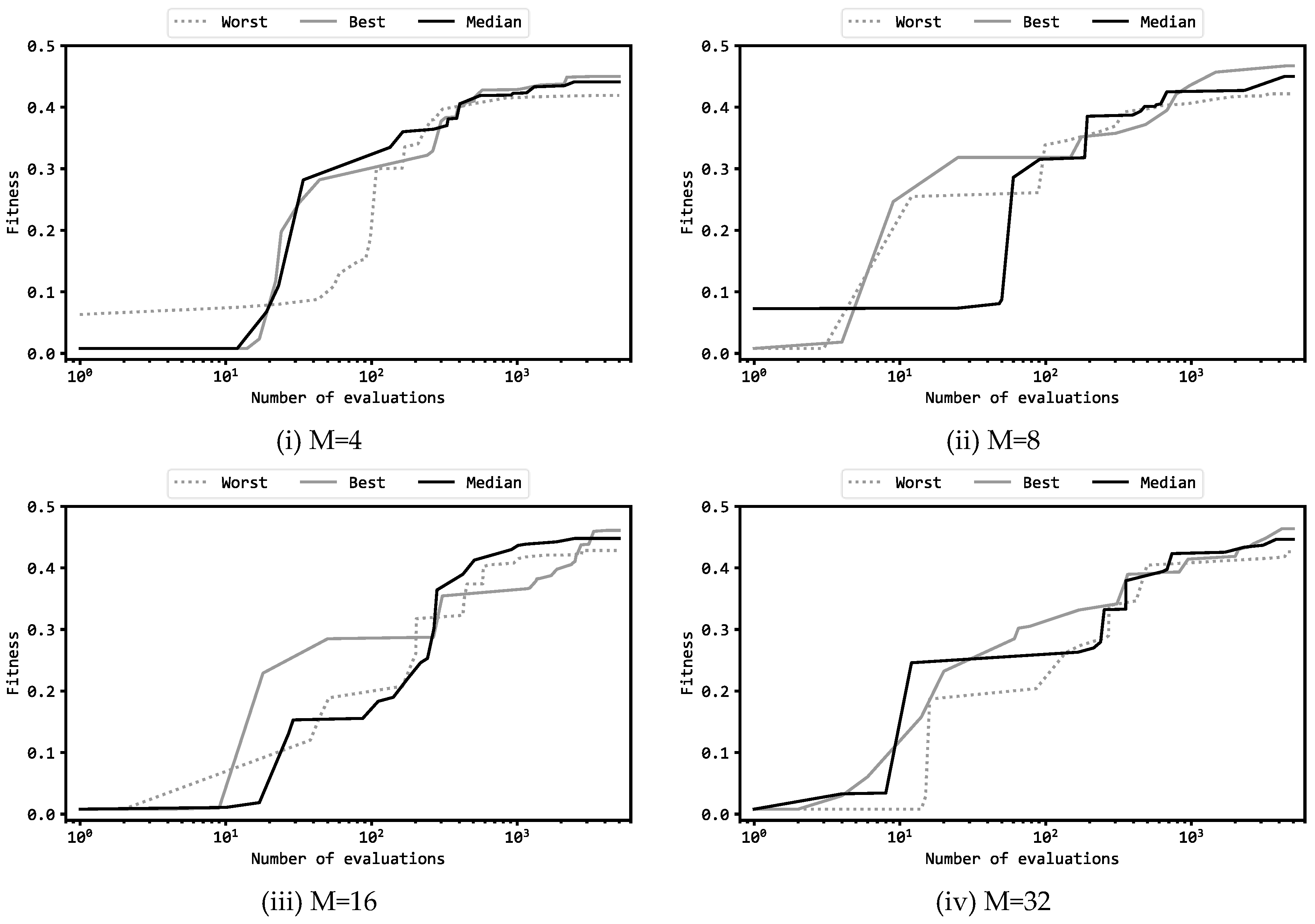
(2): Similar to the previous experiments using GA and ES, the present experiment using DE employed two configurations: maintaining a fixed number of 5000 fitness evaluations, (a) a greater number of offsprings per generation, suitable for early-stage global exploration, and (b) a greater number of generations, suitable for late-stage local exploitation. A comparative analysis of the results revealed no statistically significant difference between configurations (a) and (b) in DE. In the experiment with GA, configuration (b) demonstrated a significant superiority over (a), while in the experiment with ES, configuration (a) was significantly superior to (b). These results suggest that DE excels in maintaining a balance between global exploration and local exploitation compared to ES and GA, demonstrating robustness to configuration variations.
(3): Four different numbers of units in the hidden layer of the multilayer perceptron were compared: 4, 8, 16, and 32. The experimental results revealed that 8 units were found to be the optimal choice from the perspective of the trade-off between performance and model size. This finding aligns with previous studies using GA and ES [15,16].

The author plans to further apply and evaluate another evolutionary algorithms to the same task and compare the performance with those by DE, GA, and ES.

Acknowledgments

The author conducted this study under the Official Researcher Program of Kyoto Sangyo University.

Notes

1	https://www.gymlibrary.dev/environments/classic_control/acrobot/
2	http://youtu.be/MsNRDARXWQw
3	http://youtu.be/sxmUI8C1IBY

References

Bäck, T., & Schwefel, H. P. (1993). An overview of evolutionary algorithms for parameter optimization. Evolutionary computation, 1(1), 1-23. [CrossRef]
Fogel, D. B. (1994). An introduction to simulated evolutionary optimization. IEEE transactions on neural networks, 5(1), 3-14. [CrossRef]
Bäck, T. (1996). Evolutionary algorithms in theory and practice: evolution strategies, evolutionary programming, genetic algorithms. Oxford university press.
Eiben, Á. E., Hinterding, R., & Michalewicz, Z. (1999). Parameter control in evolutionary algorithms. IEEE transactions on evolutionary computation, 3(2), 124-141. [CrossRef]
Eiben, Á. E. , & Smith, J. E. (2015). Introduction to evolutionary computing. Springer-Verlag Berlin Heidelberg.
Schwefel, H. P. (1984). Evolution strategies: A family of non-linear optimization techniques based on imitating some principles of organic evolution. Annals of operations research, 1(2), 165-167. [CrossRef]
Beyer, H. G. , & Schwefel, H. P. (2002). Evolution strategies – a comprehensive introduction. Natural computing, 1, 3-52. [CrossRef]
Goldberg, D.E., Holland, J.H. (1988). Genetic algorithms and machine learning. Machine learning, 3, 95-99. [CrossRef]
Holland, J. H. (1992). Genetic algorithms. Scientific American, 267(1), 66-73.
Mitchell, M. (1998). An introduction to genetic algorithms. MIT press.
Sastry, K. , Goldberg, D., & Kendall, G. (2005). Genetic algorithms. Search methodologies: introductory tutorials in optimization and decision support techniques, 97-125.
Storn, R. , & Price, K. (1997). Differential evolution – a simple and efficient heuristic for global optimization over continuous spaces. Journal of global optimization, 11, 341-359. [CrossRef]
Price, K. , Storn, R. M., & Lampinen, J. A. (2006). Differential evolution: a practical approach to global optimization. Springer Science & Business Media.
Das, S. , & Suganthan, P. N. (2010). Differential evolution: a survey of the state-of-the-art. IEEE transactions on evolutionary computation, 15(1), 4-31. [CrossRef]
Okada, H. (2023). Evolutionary reinforcement learning of neural network controller for Acrobot task – Part2: genetic algorithm. Preprints.org. [CrossRef]
Okada, H. (2023). Evolutionary reinforcement learning of neural network controller for Acrobot task – Part1: evolution strategy. Preprints.org. [CrossRef]
Rumelhart, D. E. , Hinton, G. E., & Williams, R. J. (1986). Learning internal representations by error propagation. Parallel distributed processing: explorations in the microstructure of cognition, vol. 1: foundations. MIT Press, 318-362.
Collobert, R. , & Bengio, S. (2004). Links between perceptrons, MLPs and SVMs. In Proceedings of the twenty-first international conference on machine learning (ICML 04). [CrossRef]
Okada, H. (2023). A comparative study of DE, GA and ES for evolutionary reinforcement learning of neural networks in pendulum task, 25th International conference on artificial intelligence (ICAI ’23), held jointly in 2023 world congress in computer science, computer engineering, & applied computing (CSCE ’23).

Figure 1. Acrobot system1.

Figure 2. Topology of the MLP.

Figure 3. Process of Differential Evolution.

Figure 4. Learning curves of MLP with M hidden units.

Figure 5. MLP actions and the height p_y(t) in an episode.

Table 1. DE Hyperparameters.

Hyperparameters	(a)	(b)
Number of offsprings ( $λ$ )	10	50
Generations	500	100
Fitness evaluations	10 $\times$ 500=5,000	50 $\times$ 100=5,000
Scaling factor (F)	0.5	0.1
Crossover rate (CR)	0.9	0.9

Table 2. Fitness Scores among 11 Runs.

	M	Best	Worst	Average	Median
(a)	4	0.450	0.419	0.439	0.441
	8	0.467	0.422	0.448	0.450
	16	0.461	0.428	0.446	0.448
	32	0.464	0.426	0.445	0.446
(b)	4	0.464	0.433	0.445	0.443
	8	0.471	0.423	0.443	0.442
	16	0.460	0.427	0.445	0.444
	32	0.450	0.423	0.438	0.440

Disclaimer/Publisher’s Note: The statements, opinions and data contained in all publications are solely those of the individual author(s) and contributor(s) and not of MDPI and/or the editor(s). MDPI and/or the editor(s) disclaim responsibility for any injury to people or property resulting from any ideas, methods, instructions or products referred to in the content.

© 2024 by the authors. Licensee MDPI, Basel, Switzerland. This article is an open access article distributed under the terms and conditions of the Creative Commons Attribution (CC BY) license (http://creativecommons.org/licenses/by/4.0/).

Copyright: This open access article is published under a Creative Commons CC BY 4.0 license, which permit the free download, distribution, and reuse, provided that the author and preprint are cited in any reuse.