An ETD Method for Vulnerable American Options

Preprint

Article

An ETD Method for Vulnerable American Options

Altmetrics

Downloads

Views

Comments

A peer-reviewed article of this preprint also exists.

This version is not peer-reviewed

Submitted:

02 February 2024

Posted:

04 February 2024

You are already at the latest version

Alerts

Abstract

This paper introduces the exponential time differencing (ETD) technique as a numerical method to solve efficiently American vulnerable options pricing. We address several challenges, including removing cross-derivative terms through appropriate transformations, treating early-exercise opportunities using the penalty method, and substituting fixed boundary conditions with corresponding one-sided finite differences. The proposed method is shown to be both accurate and efficient through numerical experiments, which also compare the results with existing methods and analyse the numerical stability and convergence rate.

Keywords:

Subject: Computer Science and Mathematics - Computational Mathematics

1. Introduction

The Global Financial Crisis of 2007–2008 has raised concerns regarding the exposure to credit default risk in financial derivatives traded in over-the-counter (OTC) markets. In the absence of an organized exchange, option holders face the risk of default, leading to the emergence of "vulnerable options" that carry lower values compared to their non-vulnerable counterparts due to the inherent default risk.

Early studies by Johnson and Stulz [1] proposed pricing formulas for vulnerable European options under the assumption that the option represents the only liability of the involved party. Subsequent research by Klein [2] extended this work by considering the recovery of nominal claims in default and the correlation between the issuer’s asset and the underlying option asset. Further advancements [3] incorporated the Vasicek model and introduced a default boundary dependent on the option’s value. In [4], the model has been extended to accommodate default before option maturity, while Ref. [5] explores vulnerable options in incomplete markets with fluctuating interest rates.

Recently, the focus has shifted towards the pricing of American options, which offer the holder the right to exercise at any point before the expiration date. Klein and Yang [6] ventured into the realm of American vulnerable options, but a closed-form formula remained elusive. Later, Ref. [7] provided a semi-analytical solution specifically for standalone vulnerable American put options, with a focus on the early exercise boundary.

The difficulty arises in pricing vulnerable American options due to the significant discontinuity in their payoff function. Current models for these options are often based on a binomial tree method, yielding option prices and critical stock prices in tabulated form [7]. Ref. [8] utilized the two-point Geske and Johnson method to assess vulnerable American options, delivering analytical pricing formulas under risk-neutral measures. The study also delved into the price sensitivity of these options to correlations between the underlying and option writer’s assets. Further, Refs. [9,10] offered models incorporating jump-diffusion processes and correlated credit risk, respectively.

Pricing vulnerable American options poses substantial challenges due to the presence of early-exercise opportunities and the mixed derivative term in the governing nonlinear partial differential equation (PDE), which complicates numerical schemes and may result in solution instabilities [11]. To overcome these difficulties, this paper presents a novel numerical methodology that integrates multiple techniques. The penalty method, see [12] and references therein, to our knowledge, previously unexplored in the context of vulnerable American options, is employed to handle early-exercise opportunities. The resulting nonlinear PDE is then transformed into a canonical form through mixed derivative elimination [13].

The transformed PDE is solved using the Exponential Time Differencing (ETD) method [14], designed for solving ordinary differential equations (ODEs) or systems of ODEs. This method utilizes exponential integrators, known for their effectiveness in handling stiff systems characterized by solution modes with divergent decay rates. ETD techniques excel at capturing both rapid transient dynamics and slower dynamics accurately. In the context of vulnerable American options, a suitable approach is required for applying the ETD method to PDEs. The method of lines is employed to discretize space variables, such as the underlying asset price and the firm’s asset value, thereby converting the pricing PDE into a system of ODEs.

The ETD technique is then applied to this system of ODEs, efficiently yielding a stable and accurate solution for the option price. This combined approach enables the handling of the complex mixed-derivative term, which often poses numerical challenges in traditional methods. To validate the proposed method, extensive numerical experiments are conducted, comparing the results with existing approaches. Furthermore, numerical stability and convergence rate analyses reinforce the efficiency and precision of the ETD method. The findings demonstrate that the proposed method offers not only computational efficiency but also remarkable accuracy in pricing vulnerable American options.

The remainder of this paper is structured as follows. Section 2 outlines the formulation of the free-boundary PDE problem for vulnerable American options. In Section 3, the proposed methodology is detailed, encompassing the mixed-derivative removal transformation, the semi-discretization of the PDE, and the utilization of the ETD method to solve the resulting system of ODEs. Noteworthy focus is given to the solution of the default case. Section 4 presents the numerical results, including a numerical analysis of stability and convergence, as well as a comprehensive comparison with existing methods. Finally, Section 5 provides concluding remarks.

2. Vulnerable option modelling

Let us consider an American option written on the asset S which follows the risk-neutral process

\frac{d S}{S} = (r - q) d t + σ_{S} d Z_{S},

(1)

where r is the risk-free rate, q is the dividend yield,

σ_{S}

is the constant volatility of the underlying asset S,

Z_{S}

is a standard Wiener process.

If the option is traded in the over-the-counter market and there is no guaranty that participants will fulfil their obligations, the option writers become vulnerable to a counter-party credit risk, and corresponding options are known as vulnerable.

Johnson and Stulz [1] were pioneers in studying vulnerable options. They assumed that default may happen when the option price is greater than the value of the option writer’s assets. This model was extended by Klein and Inglis in [3] by allowing the option writer to hold other liabilities, but only changes in the value of the writer’s assets, including underlying asset of the option, can lead to financial distress. Later on, in [6] Klein and Yang derived the PDE formulation for vulnerable American option price considered in present study.

Let V denote the market value of the writer’s assets, which is correlated with the underlying asset price S. The risk-neutral process for V is given as follows

\frac{d V}{V} = r d t + σ_{V} d Z_{V},

(2)

where

σ_{V}

is the instantaneous standard deviation of the return on the writer’s assets,

Z_{V}

is a standard Wiener process. The instantaneous correlation coefficient between

d Z_{S}

and

d Z_{V}

ρ

Let

τ = T - t

be the time to maturity, then the vulnerable American put option price

P (τ, S; V)

is the solution of the following nonlinear PDE

\frac{\partial P}{\partial τ} = \frac{σ_{S}^{2}}{2} S^{2} \frac{\partial^{2} P}{\partial S^{2}} + \frac{σ_{V}^{2}}{2} V^{2} \frac{\partial^{2} P}{\partial V^{2}} + ρ σ_{S} σ_{V} \frac{\partial^{2} P}{\partial S \partial V} + (r - q) S \frac{\partial P}{\partial S} + r V \frac{\partial P}{\partial V} - r P,

(3)

subject to the following initial conditions

P (0, S; V) = {(S - K)}^{+} (1_{(V \geq D^{*} + K - S)} + \frac{(1 - α) V}{D^{*} + K - S} 1_{(V < D^{*} + K - S)}),

(4)

where

{(\cdot)}^{+} = max {\cdot, 0}

;

D^{*}

is the fixed default boundary such that a default occurs if the value of the option writer’s assets

V < D^{*} + {(K - S)}^{+}

. If

V \geq D^{*} + {(K - S)}^{+}

, the entire claim is paid out. Parameter

α

is the dead-weight cost related with the bankruptcy of the writer, expressed as a percentage of the value of the writer’s assets. Expression (4) is a payoff function of a vulnerable put option with strike price K, and

1_{A}

is an indicator function.

The boundary condition when

S \to \infty

for PDE put problem (3) is established as follows

lim_{S \to \infty} P (τ; S, V) = 0, τ > 0 .

(5)

Let us denote the value of corresponding non-vulnerable American option by

P_{v} (τ, S)

, which can be calculated as a solution of the Black-Scholes problem [15],

\frac{\partial P_{v}}{\partial τ} = \frac{σ_{S}^{2}}{2} S^{2} \frac{\partial^{2} P_{v}}{\partial S^{2}} + (r - q) S \frac{\partial P_{v}}{\partial S} - r P_{v}, S > S_{f} (τ),

(6)

where

S_{f} (τ)

is the unknown early exercise boundary, subject to the following initial and boundary conditions

\begin{matrix} P_{v} (0, S) & = & {(K - S)}^{+}, S_{f} (0) = K, \end{matrix}

(7)

\begin{matrix} P_{v} (τ, S_{f} (τ)) & = & K - S_{f} (τ), \frac{\partial P_{v}}{\partial S} (τ, S_{f} (τ)) = - 1, \end{matrix}

(8)

\begin{matrix} P_{v} (τ, S) & = & K - S, 0 \leq S < S_{f} (τ), \end{matrix}

(9)

\begin{matrix} lim_{S \to \infty} P_{v} (τ, S) & = & 0 . \end{matrix}

(10)

If default happens prior to maturity, the option price is calculated as follows

P (τ, S; V) = (1 - α) \frac{V}{D^{*} + P_{v} (τ, S)} P_{v} (τ, S), S \leq K, V \leq D^{*} + P_{v} (τ, S),

(11)

where

P_{v} (τ, S)

is the value of vanilla (non-vulnerable) American option defined by PDE problem (6). Expression (11) defines the amount which the holder will receive if the value of option writer’s assets does not exceed the variable default boundary prior to maturity.

If default does not happen prior to maturity (

V > D^{*} + P_{v} (τ, S)

), then the option price is a solution of PDE (3) with the conditions imposed on the optimal stopping boundary

S_{f} (τ)

[6]:

P (τ, S_{f} (τ), V) = K - S_{f} (τ), \frac{\partial P}{\partial S} (τ, S_{f} (τ), V) = - 1 .

(12)

Hence, (3) with initial conditions (4) and boundary conditions (5), is a free boundary PDE problem that can be reduced to the fixed domain problem by introducing some penalty term. In the simplest case, the penalty term is defined as follows

f (P) = μ {({(K - S)}^{+} - P (τ, S; V))}^{+},

(13)

where

μ

is some positive sufficiently large constant. This penalty term guarantees that the solution at any moment before the maturity will not be less than the payoff of the corresponding non-vulnerable option. This penalty term allows a fixed solution domain, removing the free and moving boundary imposed by the early exercise feature of the contract. Note that if

μ = 0

, PDE problem (14) reduces to the vulnerable European option.

Finally, PDE problem to be solved is

\frac{\partial P}{\partial τ} = \frac{σ_{S}^{2}}{2} S^{2} \frac{\partial^{2} P}{\partial S^{2}} + \frac{σ_{V}^{2}}{2} V^{2} \frac{\partial^{2} P}{\partial V^{2}} + ρ σ_{S} σ_{V} \frac{\partial^{2} P}{\partial S \partial V} + (r - q) S \frac{\partial P}{\partial S} + r V \frac{\partial P}{\partial V} - r P + f (P),

(14)

subject to the initial conditions (4), and boundary conditions (11).

3. Numerical solution

The PDE problem (14) with conditions (4) and (11) does not have an analytic solution and has to be solved numerically. In [6] the three-dimensional tree was used. This method is easy to implement, but computationally expensive and time-consuming for obtaining the solution not in one fixed point, but in some domain. Therefore, in present study the method of exponential time differencing proposed in [14] is employed after applying the mixed derivative terms removing transformation [13] and semi-discretization technique [16].

3.1. Mixed derivative terms removing

The presence of mixed derivative terms in a partial differential equation can lead to instabilities and inaccuracies, posing significant challenges for numerical methods. To overcome these issues, various transformation techniques have been developed to remove these mixed derivative terms. One such method, proposed in [13], is based on an

L D L^{T}

transformation of the correlation matrix, which avoids the need for iterative methods for orthogonal diagonalization of the matrix. In this paper, we adopt a similar approach to simplify the partial differential equation (14).

To begin, we apply a logarithmic transformation to the variables in the PDE, which enables us to eliminate the mixed derivative terms and reduce the problem to a more manageable form. This transformation technique has been successfully used in previous studies and provides a straightforward way to address the computational challenges posed by mixed derivative terms.

x_{1} = \frac{log (V / K)}{σ_{V}}, x_{2} = \frac{log (S / K)}{σ_{S}} .

(15)

Since the partial differential Equation (14) involves only two spatial variables, S and V, the correlation matrix and its

L D L^{T}

decomposition can be written in a simplified form

R = (\begin{matrix} 1 & ρ \\ ρ & 1 \end{matrix}) = (\begin{matrix} 1 & 0 \\ ρ & 1 \end{matrix}) (\begin{matrix} 1 & 0 \\ 0 & 1 - ρ^{2} \end{matrix}) (\begin{matrix} 1 & ρ \\ 0 & 1 \end{matrix}) = L D L^{T} .

(16)

Then, the transformation matrix C is found as

C = L^{- 1} = {(\begin{matrix} 1 & 0 \\ ρ & 1 \end{matrix})}^{- 1} = (\begin{matrix} 1 & 0 \\ - ρ & 1 \end{matrix}) .

(17)

The transformation

Y = C X

is used to remove the mixed derivative term in the PDE. Specifically, if we define

Y = {(y_{1}, y_{2})}^{T}

and

X = {(x_{1}, x_{2})}^{T}

, then we have

y_{1} = \frac{1}{σ_{V}} log (V / K), y_{2} = \frac{1}{σ_{S}} log (S / K) - \frac{ρ}{σ_{V}} log (V / K) .

(18)

The inverse transformation is

V = K e^{σ_{V} y_{1}}, S = K e^{σ_{S} (ρ y_{1} + y_{2})} .

(19)

This transformation simplifies the PDE by eliminating the mixed derivative term, resulting in a new PDE for Y. Specifically, if we substitute Y into the original PDE (14), and by denoting

U (τ, y_{1}, y_{2}) = \frac{1}{K} P (τ, S; V)

, we obtain

\frac{\partial U}{\partial τ} = \frac{1}{2} \sum_{i = 1}^{2} (d_{i}) \frac{\partial^{2} U}{\partial y_{i}^{2}} + \sum_{i = 1}^{2} (\sum_{j = 1}^{2} \frac{(r - q_{j} - σ_{j}^{2} / 2) c_{i j}}{σ_{j}}) \frac{\partial U}{\partial y_{i}} - r U + f (U),

(20)

where

d_{i}

are the diagonal elements of matrix D in (16),

c_{i j}

are the components of matrix C defined in (17), and

f (U)

is a penalty term

f (U) = μ {(U (0, y_{1}, y_{2}) - U (τ, y_{1}, y_{2}))}^{+}, μ ≫ 1 .

(21)

Hence, the transformed PDE finally takes the form

\begin{matrix} \frac{\partial U}{\partial τ} = & \frac{1}{2} \frac{\partial^{2} U}{\partial y_{1}^{2}} + \frac{(1 - ρ^{2})}{2} \frac{\partial^{2} U}{\partial y_{1}^{2}} + \frac{r - σ_{V}^{2} / 2}{σ_{V}} \frac{\partial U}{\partial y_{1}} \\ + (\frac{r - q - σ_{S}^{2} / 2}{σ_{S}} - ρ \frac{r - σ_{V}^{2} / 2}{σ_{V}}) \frac{\partial U}{\partial y_{2}} - r U + f (U) . \end{matrix}

(22)

The initial conditions (4) for V can be transformed to the new variables Y using the same transformation, resulting in the transformed initial condition for U:

U (0, y_{1}, y_{2}) = \{\begin{matrix} {(e^{σ_{S} (ρ y_{1} + y_{2})} - 1)}^{+}, & if e^{σ_{V} y_{1}} \geq \frac{D^{*}}{K} + 1 - e^{σ_{S} (ρ y_{1} + y_{2})} \\ \frac{(1 - α) e^{σ_{V} y_{1}} {(e^{σ_{S} (ρ y_{1} + y_{2})} - 1)}^{+}}{\frac{D^{*}}{K} + 1 - e^{σ_{S} (ρ y_{1} + y_{2})}}, & if e^{σ_{V} y_{1}} < \frac{D^{*}}{K} + 1 - e^{σ_{S} (ρ y_{1} + y_{2})} \end{matrix} .

(23)

To solve the transformed PDE problem, we use the ETD technique [14], which consists of two steps:

First, we apply a semi-discretization scheme to obtain a system of ordinary differential equations (ODEs) in time. In our case, we use the second-order central difference formula for space discretization, which results in a system of nonlinear ODEs.

Second, we use exponential time integration to solve the system of ODEs. The exponential time integrator is based on a splitting of the nonlinear part of the ODEs and the linear part, which can be solved exactly. This allows for an efficient and accurate numerical solution of the transformed PDE.

3.2. Semi-Discretization

Under the coordinate transformation given by (18), the solution domain

V \times S = [0, \infty) \times [0, \infty)

is transformed to the infinite domain

[y_{1}, y_{2}] = R^{2}

. Therefore, the transformed PDE (22) needs to be satisfied for any fixed pair

(y_{1}, y_{2}) \in R^{2}

. To compute a numerical solution, we consider a truncated finite domain

Ω = [y_{1_{min}}, y_{1_{max}}] \times [y_{2_{min}}, y_{2_{max}}]

and assume that (22) is fulfilled at the boundaries of

Ω

, which can then be used as the boundary conditions. Note that the rectangular domain

Ω

after applying the inverse transformation (19) becomes a non-rectangular one. However, it is always possible to choose

Ω

to represent the zone of interest.

Our goal is to construct a numerical solution for the transformed PDE problem (22) with initial conditions (23) on the truncated domain

Ω

. The ETD method is based on matrix exponentials for an exact solution of a system of ordinary differential equations (ODE). Therefore, as a preliminary step, we need to perform spatial semi-discretization.

For this purpose, we introduce a uniform mesh with step sizes in each spatial dimension given by

h_{1} = \frac{y_{1_{max}} - y_{1_{min}}}{N_{1} - 1}, h_{2} = \frac{y_{2_{max}} - y_{2_{min}}}{N_{2} - 1},

(24)

where

N_{1}

N_{2}

is the number of computational nodes in

y_{1}

and

y_{2}

, respectively. Then, the spatial nodes are

y_{i}^{j} = y_{i_{min}} + j h_{i}, j = 0, \dots, N_{i} - 1, i = 1, 2 .

(25)

Let us define an approximated solution at each spatial node by

u_{i, j} (τ) \approx U (τ, y_{1}^{i}, y_{2}^{j})

. Then, for interior nodes (

j \neq 0

j \neq N_{i} - 1

i = 1, 2

), the differential operator in

y_{1}

-dimension are discretized by using the central finite difference (FD) schemes of the second order

\begin{matrix} \frac{\partial U}{\partial y_{1}} (τ, y_{1}^{i}, y_{2}^{j}) & = & \frac{u_{i + 1, j} (τ) - u_{i - 1, j} (τ)}{2 h_{1}} + O (h_{1}^{2}), \end{matrix}

(26)

\begin{matrix} \frac{\partial^{2} U}{\partial y_{1}^{2}} (τ, y_{1}^{i}, y_{2}^{j}) & = & \frac{u_{i + 1, j} (τ) - 2 u_{i, j} (τ) + u_{i - 1, j} (τ)}{h_{1}^{2}} + O (h_{1}^{2}) . \end{matrix}

(27)

At the boundary nodes, equation (22) holds, thus, the discretization of the spatial derivatives is established by using one-sided FD of the second order,

j = 1, \dots, N_{1} - 2

\begin{matrix} \frac{\partial U}{\partial y_{1}} (τ, y_{1}^{0}, y_{2}^{j}) & = & \frac{1}{2 h_{1}} (- 3 u_{0, j} (τ) + 4 u_{1, j} (τ) - u_{2, j} (τ)) + O (h_{1}^{2}), \end{matrix}

(28)

\begin{matrix} \frac{\partial U}{\partial y_{1}} (τ, y_{1}^{N_{1} - 1}, y_{2}^{j}) & = & \frac{1}{2 h_{1}} (3 u_{N_{1} - 1, j} (τ) - 4 u_{N_{1} - 2, j} (τ) + u_{N_{1} - 3, j} (τ)) + O (h_{1}^{2}), \end{matrix}

(29)

\begin{matrix} \frac{\partial^{2} U}{\partial y_{1}^{2}} (τ, y_{1}^{0}, y_{2}^{j}) & = & \frac{1}{h_{1}^{2}} (2 u_{0, j} (τ) - 5 u_{1, j} (τ) + 4 u_{2, j} (τ) - u_{3, j} (τ)) + O (h_{1}^{2}), \end{matrix}

(30)

\begin{matrix} \frac{\partial^{2} U}{\partial y_{1}^{2}} (τ, y_{1}^{N_{1} - 1}, y_{2}^{j}) & = & \frac{1}{h_{1}^{2}} (2 u_{N_{1} - 1, j} (τ) - 5 u_{N_{1} - 2, j} (τ) + 4 u_{N_{1} - 3, j} (τ) - u_{N_{1} - 4, j} (τ)) \\ + O (h_{1}^{2}), \end{matrix}

(31)

Analogously, FD approximations can be obtained for derivatives with respect to

y_{2}

Substituting the spatial derivatives in (22) by the finite-difference approximations (26)–(28) at each spatial node

(y_{1}^{i}, y_{2}^{j})

i = 0, \dots, N_{1} - 1

j = 0, \dots, N_{2} - 1

, one gets a system of

N = N_{1} \times N_{2}

nonlinear ODEs which can be written in the following matrix form

\frac{d u}{d τ} (τ) = A u (τ) + f (u (τ)),

(32)

where

u (τ)

is a vector obtained by reshaping the matrix

{u_{i, j}}_{0 \leq i \leq N_{1} - 1, 0 \leq j \leq N_{2} - 1}

column-wise such that

u_{i, j} (τ) = u_{m} (τ), m = i + j N_{1} .

(33)

In (32),

A = {a_{i j}}_{0 \leq i, j < N}

is sparse and contains constant coefficients of the FD approximations, see [17] for details,

f (u)

is the penalty term

f (u (τ)) = μ {({(1 - s)}^{+} - u (τ))}^{+}, μ ≫ 1,

(34)

where

s

is a vector of the following components

s_{m} = exp (σ_{S} (ρ_{1}^{i} + y_{2}^{j})), m = i N_{2} + j, 0 \leq i \leq N_{1} - 1, 0 \leq j \leq N_{2} - 1 .

(35)

Let us consider the ETD method [14] for the system (32). To achieve temporal discretization, the time-step

k = \frac{T}{N_{τ}}

is chosen, and the solution at each moment

τ^{n} = n k

is obtained.

u (τ^{n + 1}) = e^{A k} u (τ^{n}) + \int_{0}^{k} e^{A s} f (u (τ^{n + 1} - s)) d s .

(36)

According to [14], Section 2.1, the integral equation (36) is equivalent to the system (32) in some given interval

[τ^{n}, τ^{n + 1}]

Approximating unknown values

u (τ^{n + 1} - s)

by known

u (τ^{n})

for

s \in [0, k]

, which has the local truncation error

O (k^{2})

[14,17], and applying the Simpsons’s quadrature rule for the integral term, one gets the explicit formula for

u (τ^{n + 1})

u (τ^{n + 1}) = e^{A k} u (τ^{n}) + \frac{k}{6} (e^{A k} + 4 e^{A k / 2} + I) f (u (τ^{n})) + O (k^{2}),

(37)

where I is the identical

N \times N

matrix. Note that approximation of the integral term by the the Simpson’s quadrature rule avoids the computation of matrix inverse, that is analytically impossible for singular matrix A and very challenging numerical task for its approximation.

Explicit formula (37) finds the solution

u (τ^{n + 1})

n = 0, \dots, N_{τ} - 1

, level-by-level starting from the initial value

u (0)

given by (23).

3.3. Default case solution

The problem of pricing vulnerable American options is highly challenging due to its multidimensionality, the presence of mixed derivative terms, early exercise options, and the possibility of default. In the event of a default prior to maturity, the option price is calculated using equation (11), while the non-vulnerable American option price is determined by solving the free-boundary PDE problem (6)–(10).

Several numerical methods have been proposed in the literature for American option pricing, including finite difference methods (FDM) [18,19], analytical approximations [20,21], and mesh-free methods [22,23], among others. In this paper, we adopt the numerical algorithm proposed in [24], which is based on the front-fixing transformation combined with explicit FDM. The algorithm computes the solution at all time-levels using a pre-determined time-step k and an appropriate spatial step-size h to ensure the stability of the numerical solution. Since the explicit FDM is used and no matrix computations are required, the algorithm is both robust and fast.

After computing the value of the non-vulnerable American option, it can be incorporated into the proposed algorithm through interpolation. In the case of default, when

S \leq K

, the vulnerable option price is computed using (11), which also requires the values of the corresponding non-vulnerable option. Therefore, for every node

(y_{1}^{i},, y_{2}^{j})

at time

τ^{n}

, the solution can be found by using the following algorithm:

Compute corresponding values S and V by using inverse transformation (19).
If $V \leq D^{*} + P_{v} (τ^{n}, S)$ (default occurs prior maturity) and $S \leq K$ , then

$u_{i, j} (τ^{n}) = (1 - α) \frac{V}{D^{*} + P_{v} (τ, S)} \frac{1}{K} P_{v} (τ, S),$
If $V > D^{*} + P_{v} (τ^{n}, S)$ (no default), then

$u_{i, j} (τ^{n}) = u_{m} (τ^{n}), m = i N_{2} + j,$

where $u_{m} (τ^{n})$ is calculated by (37).

To evaluate the performance of the proposed numerical algorithm for pricing vulnerable American options subject to default risk, we implemented the algorithm in MATLAB R2022b. In the following section, we present the numerical results obtained for different parameter values and compare them with benchmark results from the literature.

4. Numerical results

In this section, we present the results of our simulations and compare them with existing methods from the literature. We also provide an analysis of the numerical errors and convergence rates of the proposed algorithm.

The example is based on the vulnerable American option pricing problem given in [6]. We consider an option with maturity

T = 2

years, strike price

K = 200

, and volatility of the underlying asset

σ_{S} = 0.2

. The dividend yield is assumed to be zero (

q = 0

) and the interest-free rate

r = 0.05

. The option writer is assumed to be highly levered,

D^{*} = 900

V = 1000

, the volatility of the writer’s assets is

σ_{V} = 0.2

, the deadweight cost is

α = 0.25

. We assume that underlying asset S and the return on the writer’s assets V are correlated with some

ρ

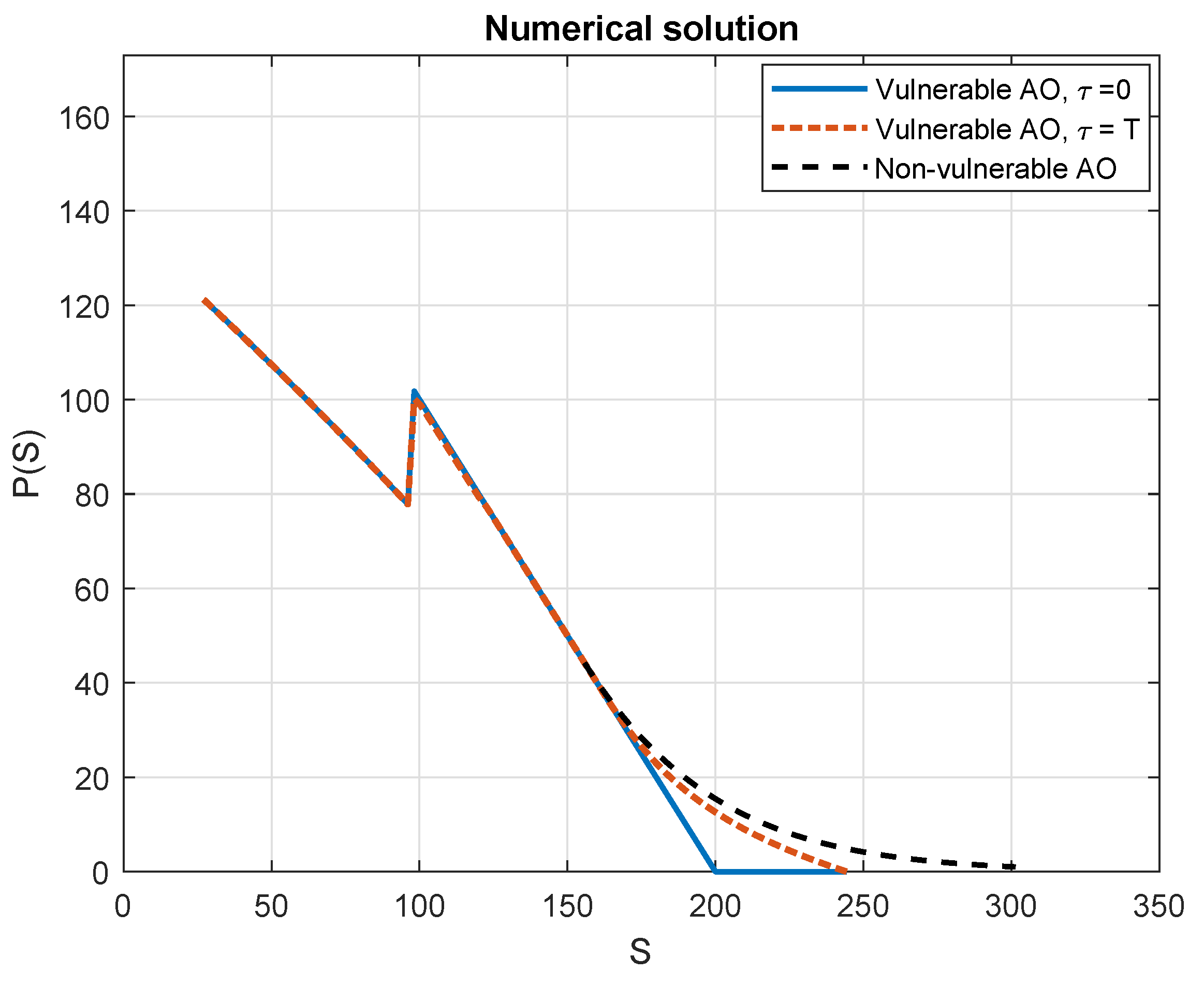
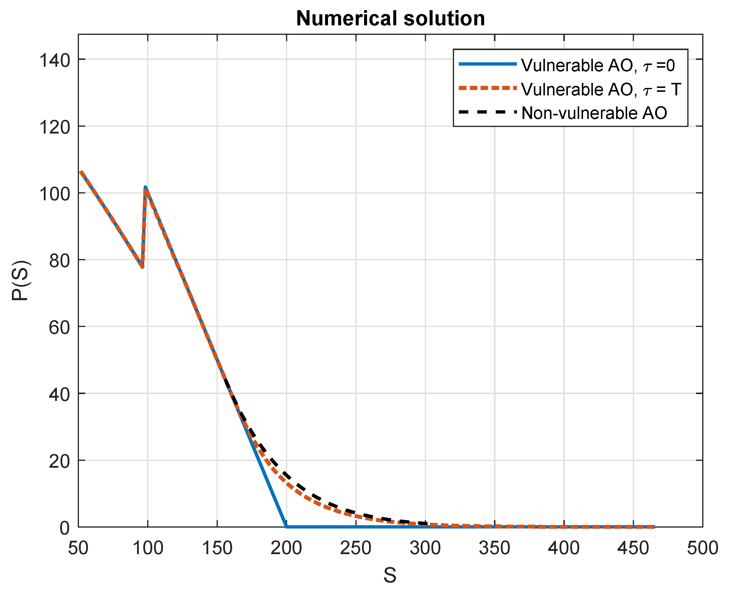
Detailed numerical solutions for scenarios when

ρ = 0

and

ρ = 0.4

have been plotted and compared with non-vulnerable options in Figure 1 and Figure 2, respectively. It’s worth noting that in cases where

ρ = 0

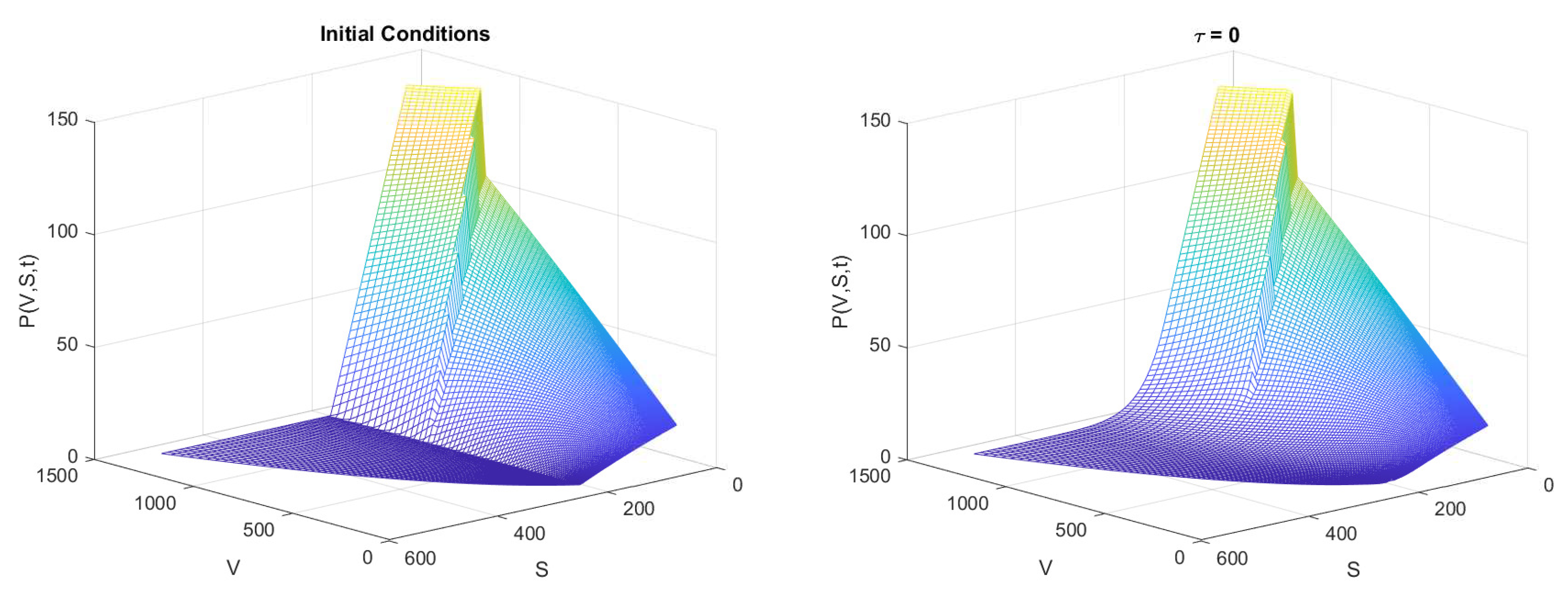
, the equation is devoid of a mixed derivative term and only the transformation as per Equation (15) is implemented, given that the correlation matrix R is identical. As for scenarios where

ρ = 0.4

, both the payoff and the numerical solution corresponding to

τ = T

are graphically represented in Figure 3.

Table 1 provides a detailed comparison of option prices for varying values of

ρ

, in accordance with the solution proposed by [6]. The computations cover a range denoted by

Ω = [- 2,, 10] \times [- 10,, 1]

, strategically selected to represent the most significant area of interest. For the discretization parameters,

N_{1}

and

N_{2}

are both set at 100, and the temporal step size is determined as

k = 0.01 \cdot min {(h_{1}, h_{2})}^{2}

. Comparing our findings with those of [6], a slight discrepancy becomes noticeable. This deviation may be attributable to the linear interpolation error that arises when determining the price at the specifically designated point S.

In all considered scenarios, it’s evident that the price of a vulnerable option is invariably lower than that of its non-vulnerable counterpart. This observation is largely ascribed to the default risk associated with the option writer, as discussed in [6].

Numerical methods require two fundamental qualities: stability and convergence. Stability, in the context of numerical methods, refers to the method’s capacity to limit errors during computation. On the other hand, convergence refers to the ability of the numerical method to approach the exact solution as the computation progresses or the step size decreases.

However, due to the intricate nature of numerical algorithms, it is often tedious and even not feasible to analytically study these properties. The complexity inherent in these algorithms often precludes a straightforward mathematical analysis of their stability and convergence characteristics.

To gain a deeper understanding of these characteristics within the context of the proposed method, we conduct a numerical investigation of both stability and convergence. This approach allows us to assess the performance of the algorithm under different conditions and verify whether it maintains the desired qualities of stability and convergence, providing valuable insights into the method’s effectiveness and reliability.

4.1. Numerical stability

First, let’s examine the aspect of numerical stability. For this purpose, we revisit the previously discussed example, fixing the spatial discretization steps at

h_{1}

and

h_{2}

. We aim to identify the parabolic mesh ratio

δ

, such that

k = δ min {h_{1}^{2}, h_{2}^{2}}

ensures a stable solution. It is evident that this ratio is influenced by the specific parameters of the problem. However, it was also observed that it depends on the penalty parameter

μ

that is related to the nonlinearity of the PDE. Therefore, in our study, we will also vary this parameter to explore its influence on stability.

For the previously discussed example, wherein

[N_{1}, N_{2}] = [50, 50]

are held constant and the values of

μ

are varied, the corresponding parabolic mesh ratios,

δ

, are tabulated in Table 2. Notably, up to

μ = 10^{3}

, the parabolic mesh ratio remains unchanged. This implies that for such values of

μ

, the stability is primarily determined by the problem parameters, and k should be selected accordingly to ensure this stability condition. However, as

μ

becomes significantly large, the influence of the penalty term starts to dominate over the problem parameters.

4.2. Numerical convergence

Drawing upon the ideas presented in [24], it is straightforward to demonstrate that the proposed scheme is consistent with the PDE problem, with a local truncation error of

O (h^{2}, k)

. In this subsection, our aim is to numerically study the convergence of the proposed method. We revisit the previous example with all but one step size held constant, which allows us to analyze the convergence with respect to the chosen variable.

We calculate the approximated option value for integer values of S in the interval

[157, 170]

, replicating the process used in the previous example. The option price computed using the binomial tree approach, as described in [6], is used as our reference value. For each simulation - that is, for each set of fixed step sizes - we compute the maximum relative error as follows

E r r o r (N_{1}, N_{2}, k) = {∥\frac{P_{ref} (S, 0) - P_{num} (S, 0)}{P_{ref} (S, 0)}∥}_{\infty} = max_{S = 157, \dots, 170} \frac{| P_{ref} (S, 0) - P_{num} (S, 0) |}{| P_{ref} (S, 0) |},

(38)

where

P_{ref}

is the reference value and

P_{num}

is the computed numerical solution.

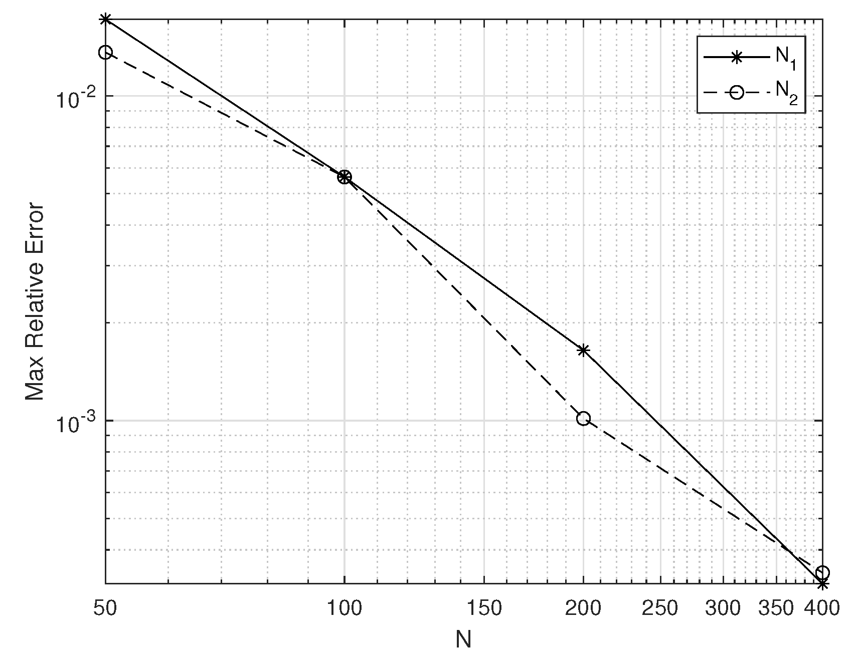
The errors for various

N_{1}

and fixed

N_{2} = 100

and

k = 10^{- 4}

, as well as corresponding errors for various

N_{2}

(fixed

N_{1} = 100

and

k = 10^{- 4}

) are plotted in Figure 4. As expected, increasing number of steps leads to more precise solution.

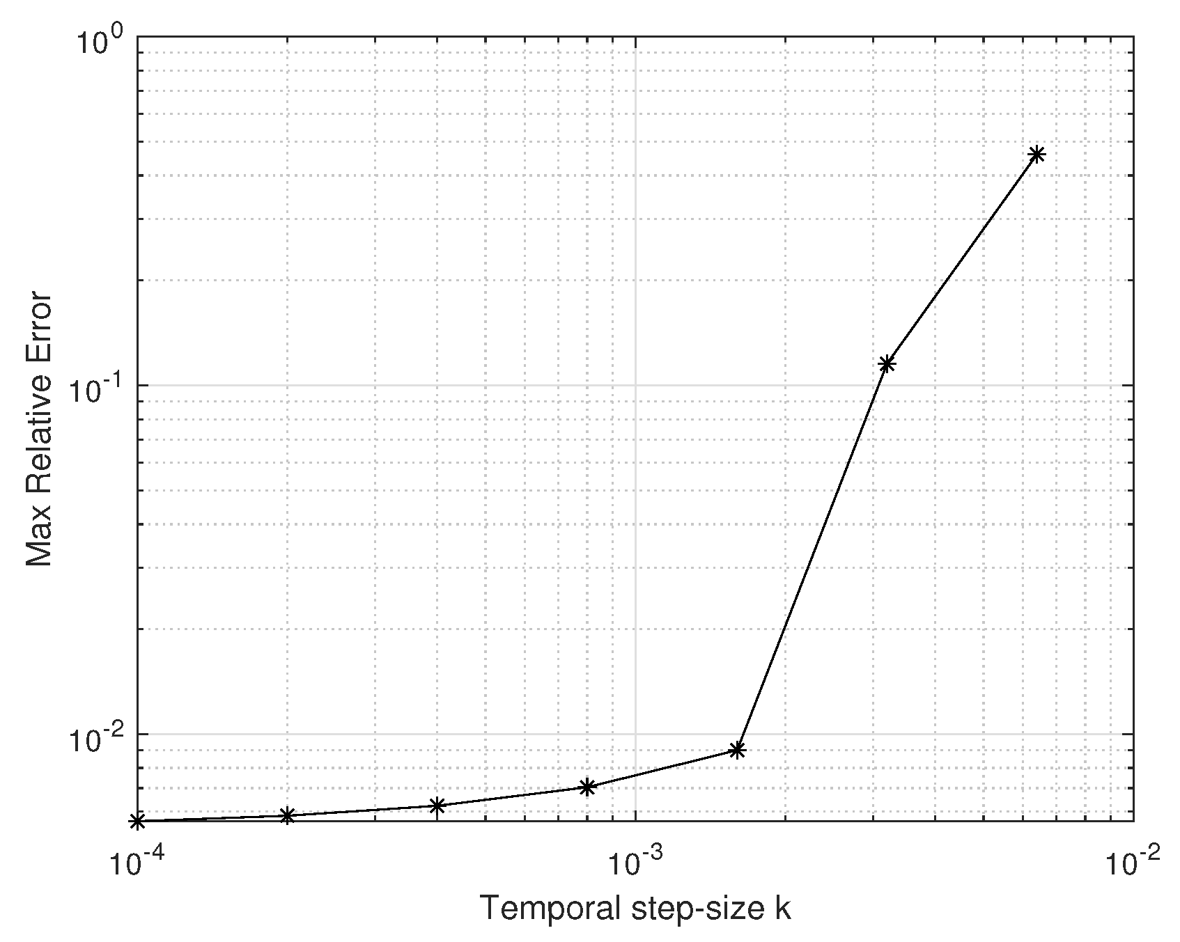
Similar plot for errors with respect to time-step k for fixed

N_{1}, N_{2} = 100

is presented in Figure 5. Note that apart from

k = 1.6 \cdot 10^{- 3}

the behaviour of error grows exponentially due to the broken stability condition. Obviously, if k is not small enough to guarantee the stability of numerical solution, the relative error increases.

Let us define the log-ratios of errors as in [26]:

γ_{N_{1}} = {log}_{2} \frac{E r r o r (N_{1}, N_{2}, k)}{E r r o r (2 N_{1}, N_{2}, k)}, γ_{N_{2}} = {log}_{2} \frac{E r r o r (N_{1}, N_{2}, k)}{E r r o r (N_{1}, 2 N_{2}, k)}

(39)

γ_{k} = {log}_{2} \frac{E r r o r (N_{1}, N_{2}, 2 k)}{E r r o r (N_{1}, N_{2}, k)} .

(40)

These ratios are calculated for all possible pairs, and the mean values are reported in Table 3.

5. Conclusions

The present study addresses the challenging problem of pricing vulnerable American options through the development of a novel numerical algorithm. We focus on the two-dimensional Black-Scholes equation, which presents several computational difficulties that must be overcome to obtain an accurate and stable solution.

One of the main challenges is the presence of a cross-derivative term in the PDE, which is caused by the correlation between the asset price and the value of the writer’s assets. This term requires a larger computational stencil and may lead to instabilities. To address this issue, we apply a cross-derivative removing transformation, which simplifies the numerical scheme and improves its stability.

Another difficulty arises from the early-exercise opportunity of American-style options, which requires the consideration of a linear complementarity problem. We propose a penalty method to convert this problem into a non-linear PDE, which can be more easily solved numerically.

The choice of appropriate boundary conditions is also crucial for obtaining an accurate solution. We take advantage of the cross-derivative removing transformation to assume that the PDE holds at the boundaries of the computational domain. As a result, we substitute fixed boundary conditions with one-sided finite difference schemes, which provide greater flexibility and versatility in the algorithm.

To solve the resulting numerical problem, we utilize the ETD method, which is a fast and easy-to-implement approach that allows us to compute the option value for a range of reasonable values of the writer’s assets. We conduct numerical experiments to compare our proposed method with other approaches in the literature and to establish its convergence rate and study the stability. Our results demonstrate the effectiveness of the proposed algorithm in accurately and efficiently pricing vulnerable American options.

In conclusion, the proposed numerical algorithm provides a valuable tool for risk management in financial markets, offering a reliable and efficient solution for pricing vulnerable American options.

Author Contributions

Conceptualization: R.C., V.N.E. and L.J.; Methodology, R.C., V.N.E. and L.J.; Validation: R.C., V.N.E. and L.J.; Formal analysis: R.C., V.N.E. and L.J.; Investigation: R.C., V.N.E. and L.J.; Writing—review and editing: R.C., V.N.E. and L.J. All authors have read and agreed to the published version of the manuscript.

Funding

This work has been partially supported by the Spanish Ministry of Economy and Competitiveness MINECO through the project PID2019-107685RB-I00 and by the Spanish State Research Agency (AEI) through the project PDC2022-133115-I00.

Institutional Review Board Statement

Not applicable.

Informed Consent Statement

Not applicable.

Data Availability Statement

Data sharing not applicable.

Conflicts of Interest

The authors declare no conflict of interest.

Abbreviations

The following abbreviations are used in this manuscript:

ETD	Exponential Time Differencing
FD	finite difference
FDM	finite difference method
PDE	Partial differential equation
ODE	Ordinary differential equation

References

Johnson H, Stulz R. The Pricing of Options with Default Risk. The Journal of Finance 1987; 42(2): 267–280. [CrossRef]
Klein PG. Pricing Black-Scholes options with correlated credit risk. Journal of Banking and Finance 1996; 20: 1211–1229.
Klein P, Inglis M. Pricing vulnerable European options when the option’s payoff can increase the risk of financial distress. tech. rep., 2001.
Liao SL, Huang HH. Pricing Black–Scholes options with correlated interest rate risk and credit risk: an extension. Quantitative Finance 2005; 5(5): 443–457. [CrossRef]
Hung MW, Liu YH. Pricing vulnerable options in incomplete markets. Journal of Futures Markets 2005; 25(2): 135–170. [CrossRef]
Klein P, Yang J. Vulnerable American options. Managerial Finance 2010; 36(5): 414–430. [CrossRef]
Zhou R. Back to CVA: the case of American option. tech. rep., 2019.
Chang LF, Hung MW. Valuation of vulnerable American options with correlated credit risk. Review of Derivatives Research 2006; 9(2): 137–165. [CrossRef]
Wang G, Wang X, Liu Z. Pricing vulnerable American put options under jump-diffusion processes. Probability in the Engineering and Informational Sciences 2016; 31: 121 - 138.
Wang S, Zhou Q, Xiao W. Pricing vulnerable American put options under jump-diffusion processes when corporate liabilities are random. Communications in Statistics - Simulation and Computation 2021: 1–21. [CrossRef]
Zvan R, Forsyth P, Vetzal K. Negative coefficients in two-factor option pricing models. The Journal of Computational Finance 2003; 7(1): 37–73. [CrossRef]
Gyulov TB, Koleva MN. Penalty method for indifference pricing of American option in a liquidity switching market. Applied Numerical Mathematics 2022; 172: 525–545. [CrossRef]
Company R, Egorova VN, Jódar L, Soleymani F. A mixed derivative terms removing method in multi-asset option pricing problems. Applied Mathematics Letters 2016; 60: 108–114. [CrossRef]
Cox SM, Matthews PC. Exponential Time Differencing for Stiff Systems. Journal of Computational Physics 2002; 176(2): 430–455. [CrossRef]
Black F, Scholes M. The Pricing of Options and Corporate Liabilities. Journal of Political Economy 1973; 81(3): 637–654.
Company R, Egorova VN, Jódar L. Conditional full stability of positivity-preserving finite difference scheme for diffusion-advection-reaction models. Journal of Computational and Applied Mathematics 2018; 341: 157–168. [CrossRef]
Company R, Egorova VN, Jódar L. A front-fixing ETD numerical method for solving jump-diffusion American option pricing problems. Mathematics and Computers in Simulation 2021; 189: 69–84. [CrossRef]
Nielsen B.F. , Skavhaug O. , Tvelto A. Penalty and front-fixing methods for the numerical solution of American option problems. Journal Of Computational Finance 2002; 5.
Tangman DY, Gopaul A, Bhuruth M. A fast high-order finite difference algorithm for pricing American options. Journal of Computational and Applied Mathematics 2008; 222(1): 17–29. [CrossRef]
Geske R, Johnson HE. The American Put Option Valued Analytically. The Journal of Finance 1984; 39(5): 1511–1524. [CrossRef]
Ju N. Pricing an American option by approximating its early exercise boundary as a multipiece exponential function. In: . 11(3). 1998 (pp. 627–646).
Hon YC, Kong SAR H, China BemryHon P. A Quasi-Radial Basis Functions Method for American Options Pricing. tech. rep., 2002.
Giribone PG, Ligato S. Option pricing via radial basis functions: Performance comparison with traditional numerical integration scheme and parameters choice for a reliable pricing. In: ; 2015.
Company R, Egorova VN, Jódar L. Solving American option pricing models by the front fixing method: Numerical analysis and computing. Abstract and Applied Analysis 2014; 2014. [CrossRef]
Hull J, White A. The impact of default risk on the prices of options and other derivative securities. tech. rep., 1995.
Company R, Egorova VN, Jódar L, Peris J. A front-fixing method for American option pricing on zero-coupon bond under the Hull and White model. In: . 45. John Wiley and Sons Ltd; 2022: 3334–3344.

Figure 1. Payoff of the vulnerable option (blue line), vulnerable American option price at

τ = 0

(orange line) for

V = 1000

and

ρ = 0.0

, non-vulnerable American option price (dashed black line).

Figure 1. Payoff of the vulnerable option (blue line), vulnerable American option price at

τ = 0

(orange line) for

V = 1000

and

ρ = 0.0

, non-vulnerable American option price (dashed black line).

Figure 2. Payoff of the vulnerable option (blue line), vulnerable American option price at

τ = 0

(orange line) for

V = 1000

and

ρ = 0.4

, non-vulnerable American option price (dashed black line).

Figure 2. Payoff of the vulnerable option (blue line), vulnerable American option price at

τ = 0

(orange line) for

V = 1000

and

ρ = 0.4

, non-vulnerable American option price (dashed black line).

Figure 3. Vulnerable American option price (

ρ = 0.4

) at the maturity (left) and at

τ = T

(right).

Figure 3. Vulnerable American option price (

ρ = 0.4

) at the maturity (left) and at

τ = T

(right).

Figure 4. Maximum relative errors with respect to number of spatial steps

N_{1}

and

N_{2}

Figure 4. Maximum relative errors with respect to number of spatial steps

N_{1}

and

N_{2}

Figure 5. Maximum relative errors with respect to temporal step-size k.

Table 1. Price of vulnerable and non-vulnerable American options for various values of correlation

ρ

. Prices in the corresponding left columns are obtained by following the three-dimensional binomial tree approach [25] and published in [6]. Prices in the corresponding right columns for each

ρ

are calculated by the proposed method.

Table 1. Price of vulnerable and non-vulnerable American options for various values of correlation

ρ

. Prices in the corresponding left columns are obtained by following the three-dimensional binomial tree approach [25] and published in [6]. Prices in the corresponding right columns for each

ρ

are calculated by the proposed method.

S	$ρ = 0.0$		$ρ = 0.4$		$ρ = 0.8$		non-vulnerable
157	43	42.99	43	42.99	43	43.00	43
158	42	41.99	42	41.99	42	42.00	42.00
159	41	40.99	41	40.99	41.01	41.03	41.08
160	40	39.99	40	39.99	40.07	40.09	40.17
161	39	38.99	39	39.02	39.14	39.13	39.27
162	38	37.99	38	38.05	38.22	38.22	38.37
163	37	37.01	37.02	37.09	37.30	37.32	37.49
164	36	36.02	36.11	36.14	36.38	36.42	36.65
165	35	35.08	35.18	35.22	35.47	35.52	35.83
166	34.03	34.14	34.26	34.31	34.56	34.63	35.01
167	33.10	33.18	33.34	33.40	33.72	33.74	34.19
168	32.16	32.30	32.43	32.52	32.84	32.85	33.40
169	31.23	31.42	31.52	31.66	31.96	31.97	32.63
170	30.39	30.55	30.63	30.79	31.11	31.12	31.89

Table 2. The approximate parabolic mesh ratio

δ

for stable numerical solution by the proposed algorithm with respect to the penalty parameter

μ

Table 2. The approximate parabolic mesh ratio

δ

for stable numerical solution by the proposed algorithm with respect to the penalty parameter

μ

$μ$	0	10	$10^{2}$	$10^{3}$	$10^{4}$
$[N_{1}, N_{2}] = [50, 50]$	$0.094$	$0.094$	$0.094$	$0.038$	$0.003$

Table 3. Numerical convergence rates in directions

y_{1}

y_{2}

and time

τ

Table 3. Numerical convergence rates in directions

y_{1}

y_{2}

and time

τ

$\bar{γ_{N_{1}}}$	1.9246
$\bar{γ_{N_{2}}}$	1.7748
$\bar{γ_{k}}$	1.0765

Disclaimer/Publisher’s Note: The statements, opinions and data contained in all publications are solely those of the individual author(s) and contributor(s) and not of MDPI and/or the editor(s). MDPI and/or the editor(s) disclaim responsibility for any injury to people or property resulting from any ideas, methods, instructions or products referred to in the content.

© 2024 by the authors. Licensee MDPI, Basel, Switzerland. This article is an open access article distributed under the terms and conditions of the Creative Commons Attribution (CC BY) license (http://creativecommons.org/licenses/by/4.0/).

Copyright: This open access article is published under a Creative Commons CC BY 4.0 license, which permit the free download, distribution, and reuse, provided that the author and preprint are cited in any reuse.

MDPI Initiatives

Important Links

Choose an area of interest and we will send you notifications of new preprints at your preferred frequency.

Disclaimer

An ETD Method for Vulnerable American Options

Abstract

1. Introduction

2. Vulnerable option modelling

3. Numerical solution

3.1. Mixed derivative terms removing

3.2. Semi-Discretization

3.3. Default case solution

4. Numerical results

4.1. Numerical stability

4.2. Numerical convergence

5. Conclusions

Author Contributions

Funding

Institutional Review Board Statement

Informed Consent Statement

Data Availability Statement

Conflicts of Interest

Abbreviations

References

MDPI Initiatives

Important Links

Subscribe