Preprint
Article

A Unified Statistical Relativistic Theory of the Generalized Brownian Motion Manifold

Altmetrics

Downloads

77

Views

28

Comments

0

A peer-reviewed article of this preprint also exists.

This version is not peer-reviewed

Submitted:

02 February 2024

Posted:

05 February 2024

You are already at the latest version

Alerts
Abstract
The current letter complements my info-geometric discoveries, especially those provided from two papers of mine. Fundamentally, the statistical relativization of the Generalized Brownian Motion Manifold. Following this innovative and unprecedented track of research will open a plethora of numerous info-geometric investigations to many unexplored related phenomena in the hope to uncover more new interpretations for the Generalized Brownian Motion Manifold from an info-geometric perspective.
Keywords: 
Subject: Computer Science and Mathematics  -   Mathematics
The reader is advised to consult([1,2]) as this letter is a continued track of research for both papers. Potentially, for the introduction and the definitions, the reader can consult[1- 16].

1. Introduction

1.1. Information Geometry

Information geometry (IG) has been widely applied in many research fields such as statistical inference, stochastic control, and neural networks .In other words, IG aims to apply the techniques of differential geometry (DG) to statistics. This means that IG’s main idea is to apply methods and techniques of non-Euclidean geometry to stochastic processes and probability theories. IG indicates that the use of Euclidian geometry technique is useful to think of a family of probability distributions as a statistical manifold (SM). Moreover, IG has been adopted for the study of statistical manifolds (SMs), where the geometric metrics gave a new description of the probability density function which plays an important role in SM and can be regarded as the coordinate system.
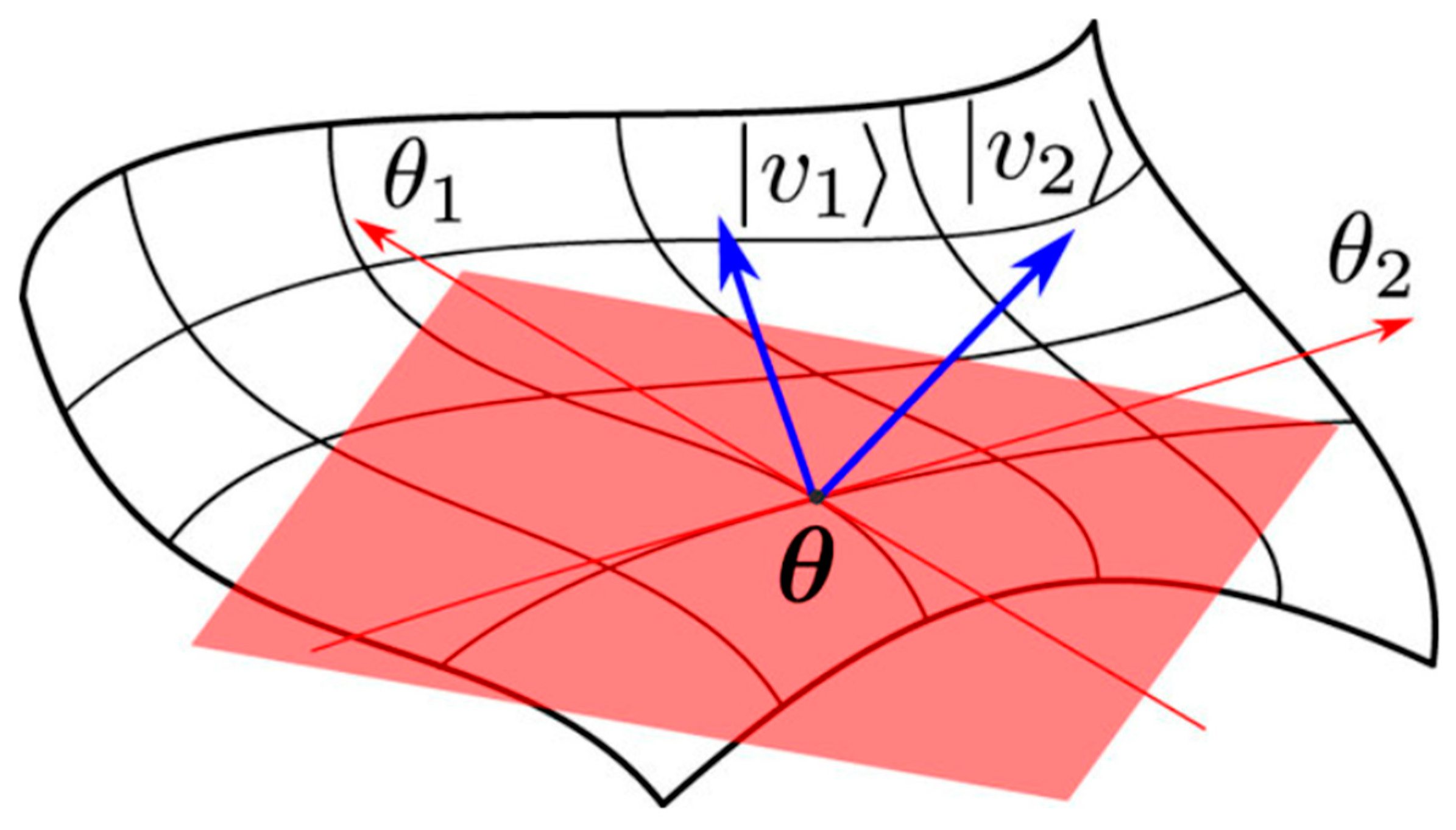
A manifold is a topological finite dimensional Cartesian space, R n , where one has an infinite-dimensional manifold. R n     could be described merely as topological space (may be defined as a set of points, along with a set of neighbourhoods for each point, satisfying a set of axioms relating points and neighbourhoods). In addition, IG supports reasoning intuitively the description of SMs. Note that although figures can be visualised (i.e., plotted in coordinate charts), they should be thought of as purely abstract figures, namely, geometric figures. One may have a higher level of appreciation of the significant importance of IG. In Figure 1, the parameter inference   θ ^     of a model from data can be interpreted as a decision-making problem: One has to decide which parameter of a family of models M = { m θ } θ ϵ Θ suits “best’’ the data, where Θ is the set of parameters { θ 1 , θ 2 , . . , θ n } of the probability density function of the distributionof the geometric manifold. IG provides a differential-geometric manifold structure M that is useful for developing decision rules.
In this paper, a study is undertaken of the geometric structure of the Generalized Brownian Motion Manifold (GBM) as well as finding its information matrix exponential (IME). The (IME) is a matrix on square matrices analogous to the ordinary exponential function. Furthermore, the Lorenzian Dynamics for (GBM) is devised.
It is used to solve systems of linear differential equations. In addition to that, the matrix exponential plays a crucial role in the theory of Lie groups. To our knowledge, the current paper is the first ever to revolutionize classic Brownian Motion Theory (BMT) by devising the Info-Geometric analysis of (GBM).
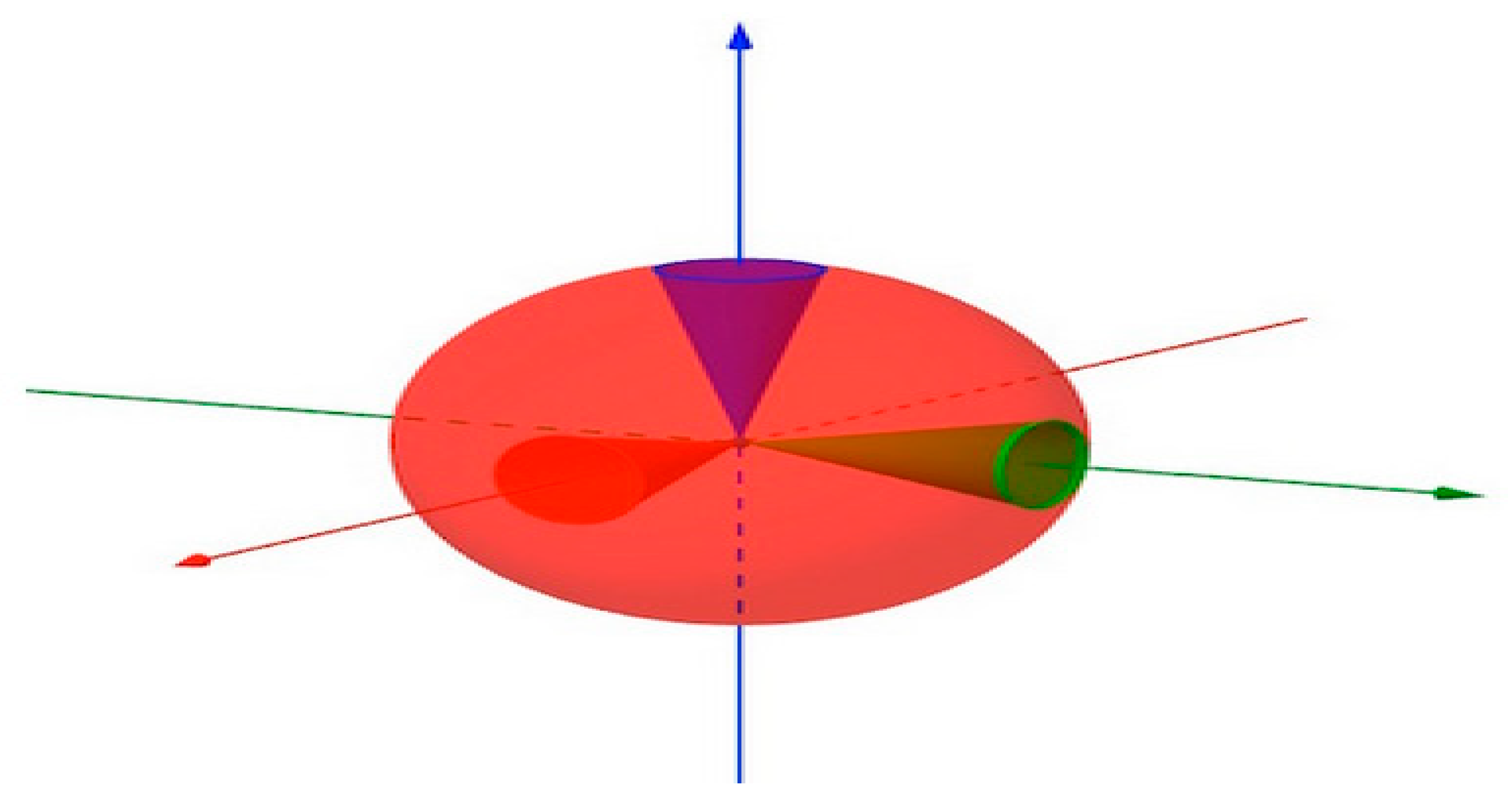
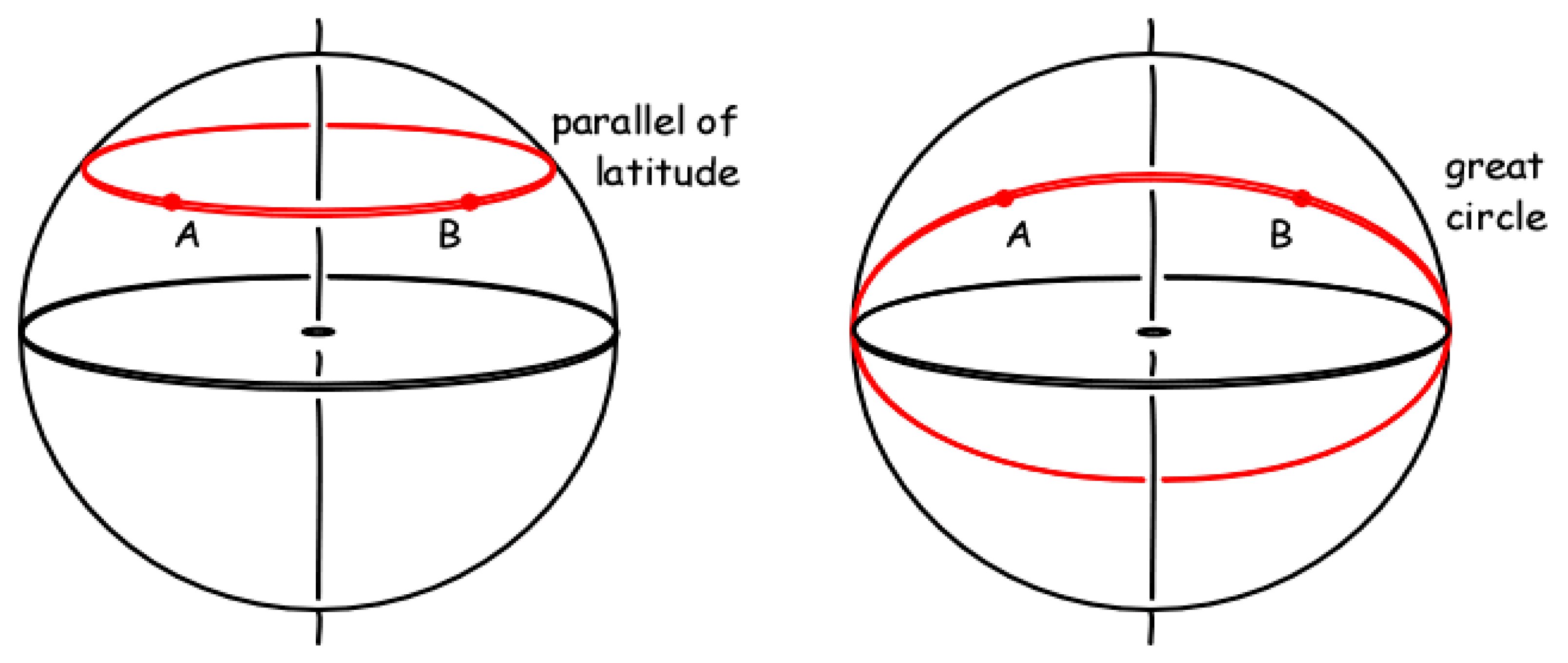
In this context, by analogy to information theory (IT), the geometric approach adopted in this paper enables the study of invariance and equivariance of figures in a coordinate-free approach (n.b., by equivariance as a concept, it is meant when there is a group acting on a pair of spaces and there is a map from functions on one to the functions on the other. In the context of this paper, Ricci curvature measures the deviation of the Riemannian metric (RM) from the standard Euclidean metric (EM) and how scalar curvature measures the deviation in the volume of a geodesic ball from the volume of an Euclidean ball of the same radius (c.f., Figure 2).
Geodesics are the analogue of straight lines in Euclidean space and possess many of the same properties as straight lines. In Einstein’s classical concept of General Relativity(GR), objects travel on a geodesic in curved space-time, which extremises the proper time between two points. Hence, the same mathematics describes both the geometry of curved spaces and the geometry of space-time. Moreover, a “straight line on a curved surface” is called a geodesic, which minimizes the distance between 2 points. In IG, the Fisher information metric (FIM) is a particular Riemannian metric (RM), which can be defined on a smooth statistical manifold (i.e., a smooth manifold whose points are probability measures defined on a common probability space). It can be used to calculate the informational difference between measurements. The FIM measures closeness of the shape between two distribution functions, it is also proportional to the amount of information that the distribution function contains about the parameter of the probability density function of the SM.

1.2. Generalized Brownian Motion (GB)

Einstein first gave a rigorous and accurate description of diffusion in simple physical systems. This description can be understood in the Eulerian framework as satisfying the diffusion equation with a constant diffusion coefficient, and in the Lagrangian framework as Brownian motion; a continuous stochastic process with stationary, independent, Gaussian increments, X t X s ,   t > s     > 0 ,   of variance δ 2 ( t s ) . In recent years several diffusive phenomena that do not fit neatly into Einstein’s framework have been discovered, and these sorts of diffusion have been collectively described as being anomalous. Examples of these phenomena include diffusion in cytoplasm and confined nanofilms, the motion of albatrosses and sharks, diffusion of polymers and dispersion in the geophysical subsurface among many others. One of the hallmarks of classical diffusion (i.e., diffusion which is described by Brownian motion and the diffusion equation with constant diffusion coefficient) is that the mean square displacement grows linearly in time.
Anomalous diffusion processes frequently do not exhibit this behaviour with a power-law mean square displacement often appearing. We should point out, however, that many diffusive processes with linear mean square displacement still are anomalous. A diverse set of models have been constructed to describe the behaviour of anomalous diffusion phenomena. These models include continuous time random walk, Lévy motion, fractional Brownian motion, and many others These models frequently have power-law mean square displacements or heavy tails. In the Lagrangian framework, they can be understood to differ from Brownian motion by having interdependent, non-stationary, or non-Gaussian increments (or some combination of the three).
The Boltzmann-Gibbs entropy can be derived by assuming that the four Shannon- Khinchin axioms hold.
For a set of discrete states, the Tsallis entropy is:
H q   =   1 q 1 ( 1 n = 1 ( p n ) q )
where   p n is the probability of being in the n t h state. In the limit q 1 , the Tsallis entropy reduces to the Boltzmann-Gibbs entropy. Assuming that the Tsallis entropy is the appropriate entropy for the system under examination, the value of q that produces an extensive entropy can be determined by examining the volume of phase space (the space of all possible system states) as a function of the system size. For example, in a classical statistical mechanical setting the system size is determined by the number of particles and the phase space volume is given by the set of all possible position and momenta coordinates ( Ω N × R 3 N ) where Ω is the box within the particles within Ω .
For a continuous random variable X , the Tsallis entropy of X is:
H q X =   1 q 1 ( 1 f X x q   d x )
where f X x is the probability density function of X .   (In a dimensional system, an issue of dimensional consistency arises the 1 in the integral in equation (1.2) have different units. However, this issue is not essential, because the 1 is a carry-over from the discrete entropy so that a system without ant randomness (one of the p n = 1 )   has zero. Shifting H q X by a constant has no impact on the employed maximum entropy).
Random variables following a q-Gaussian distribution are maximum Tsallis entropy distributions subject to holding various statistics constant (e.g., the second moment or the second q-moment). Note, however, that for fixed second moment, a q-Gaussian random variable maximizes H 2 q rather than H q . The maximum entropy properties make the q-Gaussian distribution in the context of the Tsallis entropy the analogue of the Gaussian distribution in the context of the Boltzmann-Gibbs entropy. The probability density function for a q-Gaussian is given by
f x = β C q e q ( β x 2 )
where
e q x = [ 1 + 1 q x ] 1 ( 1 q )
is called the q-exponential, C q is a normalization constant, and β > 0   is a scale parameter. In the range of extensive values of the information theoretic parameter q , 1 < q < 3 , the q-Gaussian distribution is a rescaled version of the Student’s t –distribution with ν =   3 q q 1 degrees of freedom. The scaling is such that the distributions are the same if β =   ν + 1 2 ν =   1 3 q . It is notable to state that the extensive values assigned to the information theoretic parameter q justifies the physical interpretation of Brownian Motion.
Focussing on this range, will utilize a representation of the Student’s t-distribution for a key part of the analysis below.

1.3. Random Diffusivity

Consider the stochastic differential equation:
d X t =   ν d t + D d B ( t )
where   B ( t ) is a Brownian motion, and D is a random variable that is independent of B t . Here the stochastic differential equation is regarded as being conditioned on D. If the probability density function, f D ( x ) , of D is given by
f D x = δ ( x D 0 )
then D is a constant, and the distribution of the displacement due to diffusion, X t X 0 ν t , is a Gaussian (note that the Gaussian distribution maximizes the Boltzmann-Gibbs entropy). This naturally leads to the question of whether there are distributions of D that would make the distribution of X t X 0 ν t maximize the Tsallis entropy. We will answer this question in the affirmative and explicitly construct the appropriate distribution for D.
Suppose that:
D D 0 ν V 2   g ( V )
where   V χ 2 ( ν ) is a chi-squared distribution with ν degrees of freedom and   denotes that two random variables have the same distribution. Then the distribution of X t X 0 ν t takes the form
X t X 0 ν t D t Z
D 0 t Z V ν
where Z is a standard normal random variable. At this point, we note that a Student’s t-distribution takes the form Z V ν where Z is a standard normal distribution and V is a chi-squared distribution with ν degrees of freedom. Therefore, the right-hand side of equation (1.9) is a rescaled (by a factor D 0 t ) Student’s t-distribution, or, in other words, a q-Gaussian. Hence, the distribution of X t X 0 ν t maximizes the Tsallis entropy.
By changing variables in equation (1.7), we obtain the probability density function for D:
f D x =   f V ( g 1 ( x ) )   d d x g 1 ( x ) = D 0 ( ν 4 ) ν ( ν 2 ) x ( ν 4 + 1 ) 2 ν 2 + 1 Γ ( ν 2 ) e ( ν D 0 2 x )
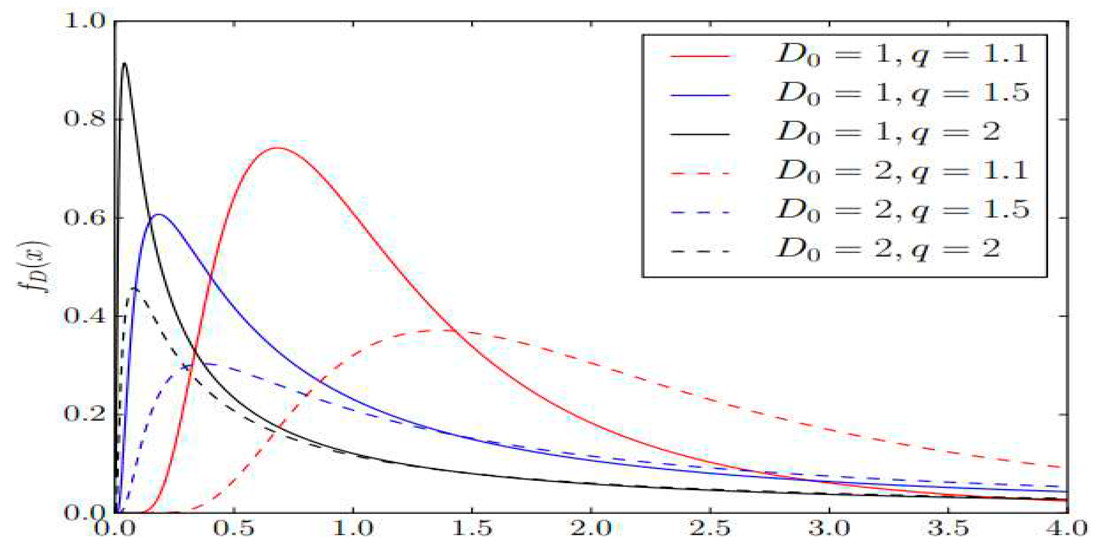
This equation can be recast in terms of q by recalling that =   3 q q 1 . Figure 3 shows several plots of f D x . Note that in the limit as q   1 + (or equivalently, ν → ∞), f D x δ ( x D 0 ) , so that equation (1.6) is satisfied in the limit. Therefore, classical advection-dispersion is recovered in the limit as q   1 + for equation (1.5). This is to be expected, since q   1 corresponds to the classical Boltzmann-Gibbs entropy, and classical advection-dispersion maximizes the Boltzmann-Gibbs entropy.
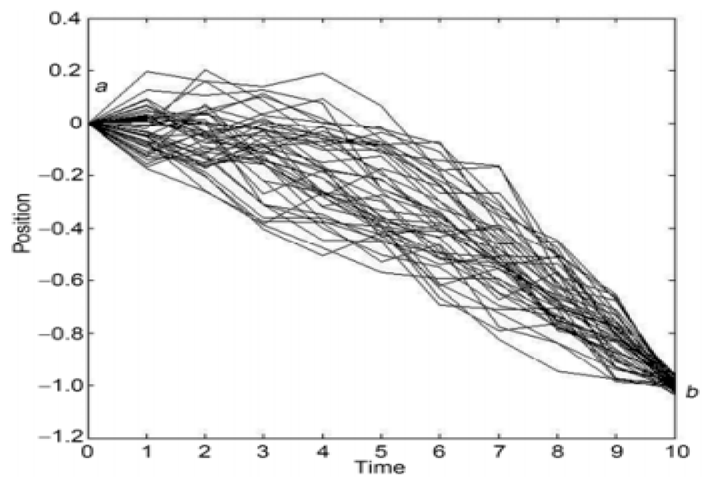
Brownian motion is an idealized approximation to actual random dynamics that has been extensively investigated over a long period time, but possibly still not thoroughly understood. Recently, Brownian, and random motion have been extended into the field of fractional Brownian motion, stochastic noise, and quantum random walks. Figure 4 shows a numerical simulation of paths (bundle) from point a to point b for particles in a constant force field such as weight. The time duration of the motion is n = 10   steps with the same unit time increment for each step. Each path is a sequence of positions { x a ,   x 1   , x 2 ,   x n 1 ,   x b }
Figure 4.
Figure 4.
Preprints 98084 g004
The main original contributions of this paper are described below.
  • The provision of the Ricci Tensor of GBM manifold
  • Revealing Ricci scalar of GBM manifold
  • Obtaining Einstein and Stress Energy tensors which unifies GBM significantly with both general and special relativity.
The rest of this paper is organised as follows: Section 1 lays out a brief introduction to Information geometry, IG and Generalized Brownian Motion , GBM. Section 2 presents preliminary definitions associated with (IG). In section 3, Ricci scalar,   R and the α c u r v a t u r e   R i e m a n n i a n Tensor, Π   s e c t i o n a l   c u r v a t u r e   t e n s o r , are calculated. In section 4, the Ricci Tensor, Υ , the c u r v a t u r e   o f   s p a c e   t i m e e i n e s t e i n   t e n s o r α n d   s t r e s s   e n e r g y   t e n s o r , Ω are calculated. Concluded remarks and future work are given in section 5.
2. Definitions[1-16]

Definition 2.1
1.Under the θ coordinate system, the α c u r v a t u r e R i e m a n n i a n Tensors,   R i j k l ( α ) (c.f.,[60]) are defined by
  R i j k l ( α ) = j Γ i k s α i Γ j k s α g s l + Γ j β , l α Γ i k β α Γ i β , l α Γ j k β α ,   i , j , k , l , s , β = 1,2 , 3 , . , n                    
where Γ i j k α =   Γ i j , s α g s k , i,j,k,s = 1,2,...,n.
2. The α R i c c i curvatures (Ricci Tensors),   R i k ( α ) are determined by)
  R i k ( α ) =   R i j k l ( α ) g j l ,   i , j , k , l = 1,2 , 3 , . , n
3.The α s e c t i o n a l   c u r v a t u r e s ,   K i j i j ( α ) are defined by (c.f., [60])
K i j i j ( α ) = R i j i j ( α ) g i i g j j ( g i j ) 2 ,   i , j = 1,2 , , n
Specifically, if n = 2 ,   the α   s e c t i o n a l   c u r v a t u r e K 1212 α = K α is called α   G a u s s i a n   c u r v a t u r e and is given by:
K α =   R 1212 ( α ) d e t g i j
4. The Ricci Tensor (c.f., [61]) is simply a contraction of the Riemannian Tensor.
5.The Ricci curvature Tensor (RCT) of an oriented Riemannian Manifold M means the extent to which the volume of a geodesic ball on the surface differs from the volume of a geodesic ball in Euclidean space.
6. The Ricci curvature (RCT) contracts the evolution of volumes under the geodesic flow. When Ricci curvature is positive, then according to the Bonnet Myers theorem the Riemannian manifold is more positively curved than a sphere and the diameter of the manifold is smaller.
Figure 4. (RCT) describes how conical regions in the manifold differ in volume from the equivalent conical regions in Euclidean space.
Preprints 98084 g005

2.2. Scalar Curvature (Ricci Scalar), R and Einestein Tensor,

The scalar curvature(Ricci Scalar), R is the contraction of Ricci Tensor.
R = R i j ( α ) g i j , i ,   j = 1,2 , 3 , .
The two-dimensional Ricci Scalar, R is twice as the Gaussian Curvature K G
R = 2 K G
The Ricci scalar R has a meaning very similar to the Gaussian Curvature. If we imagine instead of taking a circle, taking a generalized n 1 sphere, i.e. the set of all points a geodesic distance   ϵ from a given starting point x 0 ζ . We can calculate the area of this sphere in flat space, but in a curved space the area will deviate from the one we calculated by an amount proportional to the curvature. Thus, the Ricci Scalar is:
R = l i m ϵ 0 6 n ϵ 2 [ 1   A c u r v e d ( ϵ ) A f l a t ( ϵ ) ]
Ricci scalar completely captures the curvature of the surface.
The equations of motion of a classical theory like General Relativity can be derived directly from a suitable action by using the Euler-Lagrange equations, leading to the well-known Einstein equations:
G i j =     R i j ( α )   R   2 g i j = 8 π g ϖ i j c l i g h t 4    
where G i j   is the Curvature of Spacetime(Einstein tensor), ,   R i j ( α ) is the Ricci tensor of the spacetime represented by the metric g i j , R = R i j ( α ) g i j ,   i , j = 1,2 , 3 , , is the Ricci scalar or scalar curvature, g is the universal gravitational constant, c l i g h t   is the speed of light, and ϖ i j are the components of the stress-energy tensor, ϖ ,describing generically the matter-energy distributions in the spacetime.
The curvature of the n     1 dimmensional subspace orthogonal to the unit vector t is just negative two times the Einstein tensor fully contracted with the temporal vector   t . For general relativity, this means that once we choose a time direction, Einstein’s tensor tells us the scalar curvature of the corresponding spacial dimensions.

3. RICCI SCALAR, R , α C U R V A T U R E   R I E N M M A N I A N   T E N S O R , Π A N D α S E C T I O N A L   C U R V A T U R E   T E N S O R ,

3.1. Scalar Curvature (Ricci Scalar), R

Theorem 1.1 The Ricci Scalar, R of the GBM Manifold is given by:
R = 4 ν ψ 1 ν 2 4 ν 2 l n 2 3 + ψ ν 2
ψ ,   ψ 1   a r e     t h e   d i g a m m a   a n d   t r i g a m m   f u n c t i o n s ,   r e s p e c t i v e l y   ( c . f . ,   2 ) Proof
The Gaussian Curvature K G of GBM Manifold (c.f., [2]) is given by:
K G =   2 ( ν ψ 1 ν 2 4 ) ν 2 ( l n 2 3 + ψ ( ν 2 ) )
Following (2.6), it holds that:
R = 2 K G = 4 ( ν ψ 1 ν 2 4 ) ν 2 ( l n 2 3 + ψ ( ν 2 ) )
This proves our theorem.

3.2 T h e α C U R V A T U R E   R I E N M M A N I A N   T E N S O R , Π

In this section, α C u r v a t u r e R i e n m m a n i a n T e n s o r , Π is obtained. This unifies GBM manifold with Riemannian geometry, which will be used to devise the α s e c t i o n a l c u r v a t u r e s tensor, .
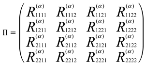
Theorem 3.2 The α C u r v a t u r e R i e n m m a n i a n T e n s o r , Π of the GBM Manifold is given by:
Preprints 98084 i001
where
  R 1111 α =   R 1112 α =   R 1121 α =   R 1122 α =   R 2211 α =   R 2212 α =   R 2221 α =   R 2222 α = 0
  R 1211 α = 2 1 α ν ψ 1 ν 2 5 2   1 ν 3 + 1 8 ψ 2 ν 2 + ν + 1 16 ψ 3 ν 2 ν ψ 1 ν 2 5 ν + 1 1 ν 2 + 1 8 ψ 2 ν 2 ψ 1 ν 2 + ν 2 ψ 2 ν 2 + ν ψ 1 ν 2 5 4 D 0 2 ( 1 ν + 1 4 ψ 1 ( ν 2 ) 1 4 D 0 ) + 1 α ν ψ 1 ν 2 5 1 ν 2 + 1 8 ψ 2 ν 2 8 D 0 ( 1 D 0 1 ) ]
  R 1212 α = [ ( D 0 ν ) ( 1 α ) ( 4 D 0 2 ( ν ψ 1 ν 2 5 ) 2 1 2 D 0 ψ 1 ν 2 + ν 2 ψ 2 ν 2 + ν ψ 1 ν 2 5 1 ν 2 ν 2 ψ 2 ν 2 + 1 ν 1 4 ψ 1 ν 2 ψ 1 ν 2 + ν 2 ψ 2 ν 2 + ( ( 1 α ) 2 64 Δ D 0 4 ) ( ( ν 2 D 0 ) ( 1 ν 2 + 1 8 ψ 2 ν 2 ) + ( 1 ν 1 4 ψ 1 ν 2
))] (
Where ψ 2 ( z ) = d d z ( ψ 1 )
  R 1221 ( α ) = 1 α 1 2 ν ψ 1 ν 2 5 D 0 2 1 2 D 0 2 ( [ ( 2 ψ 1 ν 2 ν ψ 2 ν 2 ) D 0 ] ν ψ 1 ν 2 5 [ ( 9 2 ν ψ 1 ν 2 ) ) ν D 0 ] ψ 1 ν 2 + ν 2 ψ 2 ν 2 ν ψ 1 ν 2 5 ( 1 ν + 1 4 ψ 1 ( ν 2 ) 1 4 D 0 ) + 1 α 4 D 0 2 1 ν + 1 4 ψ 1 ν 2 ν ψ 1 ν 2 5 + [ ν ( 1 ν 2 + 1 8 ψ 2 ( ν 2 ) ) 2 ν ψ 1 ν 2 5 ]
R 1222 ( α ) = 1 α D 0 2 ν ψ 1 ν 2 5 2 5 ν ψ 1 ν 2 2 + 1 2 ν ψ 2 ν 2 2 ψ 1 ν 2 D 0 1 ν ψ 1 ν 2 5 9 2 ν ψ 1 ν 2 D 0 ν ψ 1 ν 2 + ν 2 ψ 2 ν 2 1 4 D 0 ν 4 D 0 2 + 1 α ν ψ 1 ν 2 5 1 4 1 ν + 1 4 ψ 1 ν 2 + [ ν 8 D 0 2 ( 9 2 ν ψ 1 ν 2 ) ]            
  R 2111 ( α ) = 2 1 α ν ψ 1 ν 2 5 2 ψ 1 ν 2 + ν 2 ψ 2 ν 2 + 1 ν 2 + 1 4 ψ 2 ν 2 D 0 ν ψ 1 ν 2 5 [ ν ψ 1 ν 2 5 + 1 ν + 1 4 ψ 1 ν 2 D 0 ] ψ 1 ν 2 + ν 2 ψ 2 ν 2 ) ( 1 ν + 1 4 ψ 1 ν 2 1 4 D 0 ) D 0 + 1 α ν ψ 1 ν 2 5 64 D 0 2 1 ν 2 + 1 8 ψ 2 ν 2 D 0 2 1 ν + 1 4 ψ 1 ν 2
R 2112 ( α ) = 1 α ν ψ 1 ν 2 5 2 4 1 ν 2 + 1 8 ψ 2 ν 2 D 0 ν ψ 1 ν 2 5 1 + 4 1 ν + 1 4 ψ 1 ν 2 D 0 ψ 1 ν 2 + ν 2 ψ 2 ν 2 1 4 D 0 + ν 4 D 0 2 + ν ψ 1 ν 2 5 1 α 16 D 0 3 ( 4 D 0 1 ν 2 + 1 8 ψ 2 ν 2 [ 1 8 ν 1 ν + 1 4 ψ 1 ν 2 ]
  R 2121 α = α 1 ν ψ 1 ν 2 5 2 ν ψ 1 ν 2 5 + ν (   ψ 1 ν 2 + ν 2 ψ 2 ν 2 ) 2 D 0 2 + [ ν ψ 1 ν 2 5 2 ψ 1 ν 2 + ν ψ 2 ν 2 + ( 9 2 ν ψ 1 ν 2 ψ 1 ν 2 + ν 2 ψ 2 ν 2 ] 2 D 0 9 2 ν ψ 1 ν 2 [ ν ψ 1 ν 2 5 2 D 0 2 ] 1 ν + 1 4 ψ 1 ν 2 1 4 D 0 + ν ψ 1 ν 2 5 1 α 32 D 0 2 ν ψ 2 ν 2 + 2 ψ 1 ν 2
  R 2122 ( α )     = 1 α 2 D 0 2 ν ψ 1 ν 2 5 2 2 ν ψ 1 ν 2 ν 2 ψ 2 ν 2 D 0 1 ) ν ψ 1 ν 2 5 9 2 ν ψ 1 ν 2 D 0 ν ) ψ 1 ν 2 + ν 2 ψ 2 ν 2 + [ ν ψ 1 ν 2 5 ] 1 4 D 0 + ν 4 D 0 2 + 1 α 4 9 2 ν ψ 1 ν 2 D 0 [ 1 ν + 1 4 ψ 1 ν 2 ]
Proof
It is obtained that the Fisher Information Matrix of GBM Manifold, [ g i j ] (c.f., [1]) is determined by:
g i j = 1 ν + 1 4 ψ 1 ( ν 2 ) 1 4 D 0 1 4 D 0 ν 4 D 0 2 ,   w i t h   Δ = det g i j = 1 16 D 0 2 ν ψ 1 ν 2 5 0 ( c . f . , [ 1 ] )
Moreover, the reader can check that the α connections of the GBM manifold (c.f., [1]) given by
Γ 11,1   ( α ) = 1 α 2 ( 1 ν 2 + 1 8 ψ 2 ( ν 2 ) )
Γ 11,2 ( α ) = Γ 12,1 ( α ) = Γ 21,1 ( α ) = 0
Γ 12,2 ( α ) = 1 α 8 D 0 2 = Γ 22,1 ( α ) = Γ 21,2 ( α )
Γ 22,2 ( α ) =   α 1 ν 4 D 0 3
Γ 11 1 α = 1 α ν 8 Δ D 0 2 ( 1 ν 2 + 1 8 ψ 2 ( ν 2 ) ) ,   Γ 11 1 0 = ν 8 Δ D 0 2 ( 1 ν 2 + 1 8 ψ 2 ( ν 2 ) )
Γ 12 1 α = Γ 21 1 α = 1 α 32 Δ D 0 3   ,   Γ 12 1 0 = Γ 21 1 0 = 1 32 Δ D 0 3
Γ 22 1 α = α 1 ν 32 Δ D 0 4 ,   Γ 22 1 0 = ν 32 Δ D 0 4
Γ 11 2 α = 1 α 8 Δ D 0 2 1 ν 2 + 1 8 ψ 2 ν 2 ,     Γ 11 2 0 = 1 8 Δ D 0 2 ( 1 ν 2 + 1 8 ψ 2 ( ν 2 ) )
Γ 12 2 α = Γ 21 2 α = 1 α 8 D 0 2 1 ν + 1 4 ψ 1 ν 2 ,   Γ 12 2 0 = Γ 21 2 0 = 1 8 D 0 2 1 ν + 1 4 ψ 1 ν 2
Γ 22 2 α = 1 α 32 Δ D 0 3 9 2 ν ψ 1 ν 2 ,   Γ 22 2 ( 0 ) = 1 32 Δ D 0 3 ( 9 2 ν ψ 1 ν 2 )
It can be verified that:
  R 1111 α =   R 2222 α =   R 1112 α =   R 1121 α =   R 1122 α =   R 2211 α =   R 2212 α =   R 2221 α = 0
  R 1211 α = ν ( Γ 11 1 α + Γ 11 2 α ) D 0 ( Γ 21 1 α + Γ 21 2 α ) ( g 11 + g 21 ) + [ Γ 21,1 α Γ 11 1 α + Γ 22,1 α Γ 11 2 α ] [ Γ 11,1 α Γ 21 1 α + Γ 12,1 α Γ 21 2 α ] = ν ( 2 1 α ν ν ψ 1 ν 2 5 ( 1 ν 2 + 1 8 ψ 2 ( ν 2 ) ) + 2 1 α ν ψ 1 ν 2 5 ( 1 ν 2 + 1 8 ψ 2 ( ν 2 ) ) ) D 0 ( 1 α 32 Δ D 0 3 + 2 1 α ν ψ 1 ν 2 5 1 ν + 1 4 ψ 1 ν 2 ) ( 1 ν + 1 4 ψ 1 ( ν 2 ) 1 4 D 0 ) + 1 α 4 D 0 2 1 α ν ψ 1 ν 2 5 1 ν 2 + 1 8 ψ 2 ν 2 [ 1 α 2 ( 1 ν 2 + 1 8 ψ 2 ( ν 2 ) ) 1 α 2 D 0 ν ψ 1 ν 2 5 ] = 2 1 α ν ψ 1 ν 2 5 2   1 ν 3 + 1 8 ψ 2 ν 2 + ν + 1 16 ψ 3 ν 2 ν ψ 1 ν 2 5 ν + 1 1 ν 2 + 1 8 ψ 2 ν 2 ψ 1 ν 2 + ν 2 ψ 2 ν 2 + ν ψ 1 ν 2 5 4 D 0 2 ( 1 ν + 1 4 ψ 1 ( ν 2 ) 1 4 D 0 ) + 1 α ν ψ 1 ν 2 5 1 ν 2 + 1 8 ψ 2 ν 2 8 D 0 ( 1 D 0 1 ) ]
  R 1212 α = [ ( D 0 ν ) ( 1 α ) ( 4 D 0 2 ( ν ψ 1 ν 2 5 ) 2 1 2 D 0 ψ 1 ν 2 + ν 2 ψ 2 ν 2 + ν ψ 1 ν 2 5 1 ν 2 ν 2 ψ 2 ν 2 + 1 ν 1 4 ψ 1 ν 2 ψ 1 ν 2 + ν 2 ψ 2 ν 2 + ( ( 1 α ) 2 64 Δ D 0 4 ) ( ( ν 2 D 0 ) ( 1 ν 2 + 1 8 ψ 2 ν 2 ) + ( 1 ν 1 4 ψ 1 ν 2
))]
  R 1221 ( α ) = 2 ( Γ 12 1 α + Γ 12 2 α ) 1 ( Γ 22 1 α + Γ 22 2 α ) ( g 11 + g 21 ) + [ Γ 21,1 α Γ 12 1 α + Γ 22,1 α Γ 12 2 α ] [ Γ 11,1 α Γ 22 1 α + Γ 12,1 α Γ 22 2 α ] = 1 α 1 2 ν ψ 1 ν 2 5 D 0 2 1 2 D 0 2 ( [ ( 2 ψ 1 ν 2 ν ψ 2 ν 2 ) D 0 ] ν ψ 1 ν 2 5 [ ( 9 2 ν ψ 1 ν 2 ) ) ν D 0 ] ψ 1 ν 2 + ν 2 ψ 2 ν 2 ν ψ 1 ν 2 5 ( 1 ν + 1 4 ψ 1 ( ν 2 ) 1 4 D 0 ) + 1 α 4 D 0 2 1 ν + 1 4 ψ 1 ν 2 ν ψ 1 ν 2 5 + [ ν ( 1 ν 2 + 1 8 ψ 2 ( ν 2 ) ) 2 ν ψ 1 ν 2 5 ]
Engaging the same procedure, the remaining tensorial components will follow. This completes the proof of our theorem.
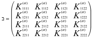
Theorem 3.3 The α S e c t i o n a l   C u r v a t u r e   T e n s o r , of the GBM Manifold is given by:
Preprints 98084 i002
where
  K 1111 α =   K 1112 α =   K 1121 α =   K 1122 α =   K 2211 α =   K 2212 α =   K 2221 α =   K 2222 α = 0
  K 1211 α = 32 1 α D 0 2 ν ψ 1 ν 2 5 3   1 ν 3 + 1 8 ψ 2 ν 2 + ν + 1 16 ψ 3 ν 2 ν ψ 1 ν 2 5 ν + 1 1 ν 2 + 1 8 ψ 2 ν 2 ψ 1 ν 2 + ν 2 ψ 2 ν 2 + ν ψ 1 ν 2 5 4 D 0 2 ( 1 ν + 1 4 ψ 1 ( ν 2 ) 1 4 D 0 ) + 1 α ν ψ 1 ν 2 5 1 ν 2 + 1 8 ψ 2 ν 2 8 D 0 ( 1 D 0 1 ) ]
  K 1212 α = [ 4 ( D 0 ν ) ( 1 α ) ( ν ψ 1 ν 2 5 ) 3 1 2 D 0 ψ 1 ν 2 + ν 2 ψ 2 ν 2 + ν ψ 1 ν 2 5 1 ν 2 ν 2 ψ 2 ν 2 + 1 ν 1 4 ψ 1 ν 2 ψ 1 ν 2 + ν 2 ψ 2 ν 2 + ( ( 1 α ) 2 64 Δ D 0 4 ) ( ( ν 2 D 0 ) ( 1 ν 2 + 1 8 ψ 2 ν 2 ) + ( 1 ν 1 4 ψ 1 ν 2
))]
  K 1221 ( α ) = 16 D 0 2 1 α ( ν ψ 1 ν 2 5 ) 3 1 2 ν ψ 1 ν 2 5 D 0 2 1 2 D 0 2 ( [ ( 2 ψ 1 ν 2 ν ψ 2 ν 2 ) D 0 ] ν ψ 1 ν 2 5 [ ( 9 2 ν ψ 1 ν 2 ) ) ν D 0 ] ψ 1 ν 2 + ν 2 ψ 2 ν 2 ν ψ 1 ν 2 5 ( 1 ν + 1 4 ψ 1 ( ν 2 ) 1 4 D 0 ) + 1 α 4 D 0 2 1 ν + 1 4 ψ 1 ν 2 ν ψ 1 ν 2 5 + [ ν ( 1 ν 2 + 1 8 ψ 2 ( ν 2 ) ) 2 ν ψ 1 ν 2 5 ]
K 1222 ( α ) = 16 1 α ν ψ 1 ν 2 5 3 5 ν ψ 1 ν 2 2 + 1 2 ν ψ 2 ν 2 2 ψ 1 ν 2 D 0 1 ν ψ 1 ν 2 5 9 2 ν ψ 1 ν 2 D 0 ν ψ 1 ν 2 + ν 2 ψ 2 ν 2 1 4 D 0 ν 4 D 0 2 + 1 α ν ψ 1 ν 2 5 1 4 1 ν + 1 4 ψ 1 ν 2 + [ ν 8 D 0 2 ( 9 2 ν ψ 1 ν 2 ) ]                
  K 2111 ( α ) = 32 D 0 2 1 α ν ψ 1 ν 2 5 3 ψ 1 ν 2 + ν 2 ψ 2 ν 2 + 1 ν 2 + 1 4 ψ 2 ν 2 D 0 ν ψ 1 ν 2 5 [ ν ψ 1 ν 2 5 + 1 ν + 1 4 ψ 1 ν 2 D 0 ] ψ 1 ν 2 + ν 2 ψ 2 ν 2 ) ( 1 ν + 1 4 ψ 1 ν 2 1 4 D 0 ) D 0 + 1 α ν ψ 1 ν 2 5 64 D 0 2 1 ν 2 + 1 8 ψ 2 ν 2 D 0 2 1 ν + 1 4 ψ 1 ν 2
K 2112 ( α ) = 16 D 0 2 1 α ν ψ 1 ν 2 5 3 4 1 ν 2 + 1 8 ψ 2 ν 2 D 0 ν ψ 1 ν 2 5 1 + 4 1 ν + 1 4 ψ 1 ν 2 D 0 ψ 1 ν 2 + ν 2 ψ 2 ν 2 1 4 D 0 + ν 4 D 0 2 + ν ψ 1 ν 2 5 1 α 16 D 0 3 ( 4 D 0 1 ν 2 + 1 8 ψ 2 ν 2 [ 1 8 ν 1 ν + 1 4 ψ 1 ν 2 ]
  K 2121 α = 16 D 0 2 α 1 ν ψ 1 ν 2 5 3 ν ψ 1 ν 2 5 + ν (   ψ 1 ν 2 + ν 2 ψ 2 ν 2 ) 2 D 0 2 + [ ν ψ 1 ν 2 5 2 ψ 1 ν 2 + ν ψ 2 ν 2 + ( 9 2 ν ψ 1 ν 2 ψ 1 ν 2 + ν 2 ψ 2 ν 2 ] 2 D 0 9 2 ν ψ 1 ν 2 [ ν ψ 1 ν 2 5 2 D 0 2 ] 1 ν + 1 4 ψ 1 ν 2 1 4 D 0 + ν ψ 1 ν 2 5 1 α 32 D 0 2 ν ψ 2 ν 2 + 2 ψ 1 ν 2
  K 2122 ( α )     = 8 1 α ν ψ 1 ν 2 5 3 2 ν ψ 1 ν 2 ν 2 ψ 2 ν 2 D 0 1 ) ν ψ 1 ν 2 5 9 2 ν ψ 1 ν 2 D 0 ν ) ψ 1 ν 2 + ν 2 ψ 2 ν 2 + [ ν ψ 1 ν 2 5 ] 1 4 D 0 + ν 4 D 0 2 + 1 α 4 9 2 ν ψ 1 ν 2 D 0 [ 1 ν + 1 4 ψ 1 ν 2 ]
Proof
Engaging
K i j i j ( α ) = R i j i j ( α ) ,   i , j = 1,2
a n d (3.4)-(3.12), the proofs are immediate.

4. RICCI CURVATURE TENSOR, Υ , C U R V A T U R E O F S P A C E T I M E (EINESTEIN T E N S O R ) , AND S T R E S S E N E R G Y T E N S O R , Ω O F G B M M A N I F O L D

4.1. Ricci, Einstein, and Stress Energy Tensors

Theorem 4.1 The Ricci Tensor corresponding to the curvature parameter α = 0 , Υ of the GBM manifold is determined by:
Υ = R 11 ( 0 ) R 12 ( 0 ) R 21 ( 0 ) R 22 ( 0 )                                                                                                
w h e r e
R 11 ( 0 ) = 4 D 0 ( ν ψ 1 ν 2 5 )   [ 1 4 ψ 1 ν 2 1 4 D 0 1 ν ψ 1 ν 2 + ν 2 ψ 2 ν 2 D 0 ν ψ 1 ν 2 5 2 + 1 ν 2 + 1 8 ψ 2 ν 2 ψ 2 ν 2 + 8 ν 2 1 D 0 2 ν ψ 1 ν 2 5 + 4 ν ν ψ 1 ν 2 5 D 0 ν 4 D 0 2 ν ψ 1 ν 2 5 2 1 2 D 0 ψ 1 ν 2 + ν 2 ψ 2 ν 2 + ν ψ 1 ν 2 5 1 ν 2 ν 2 ψ 2 ν 2 + 1 ν 1 4 ψ 1 ν 2 ψ 1 ν 2 + ν 2 ψ 2 ν 2 + 4 ( ν 2 D 0 ( 1 ν 2 + 1 8 ψ 2 ν 2 + 1 ν 1 4 ψ 1 ν 2 ) D 0 2 ν ψ 1 ν 2 5 ( c . f . , [ 1 ] )
R 12 ( 0 ) = We have
  R i k ( α ) =   R i j k l ( α ) g j l ,   i , j , k , l = 1,2 , 3 , . , n
  R 12 ( 0 )                   = 1 2 ν ψ 1 ν 2 5 D 0 2 1 2 D 0 2 ( [ ( 2 ψ 1 ν 2 ν ψ 2 ν 2 ) D 0 ] ν ψ 1 ν 2 5 [ ( 9 2 ν ψ 1 ν 2 ) ) ν D 0 ] ψ 1 ν 2 + ν 2 ψ 2 ν 2 ν ψ 1 ν 2 5 ( 1 ν + 1 4 ψ 1 ( ν 2 ) 1 4 D 0 ) + 1 4 D 0 2 1 ν + 1 4 ψ 1 ν 2 ν ψ 1 ν 2 5 + [ ν ( 1 ν 2 + 1 8 ψ 2 ( ν 2 ) ) 2 ν ψ 1 ν 2 5 ] 4 D 0 ν ψ 1 ν 2 5 + 16 ( 1 ν + 1 4 ψ 1 ( ν 2 ) ν ψ 1 ν 2 5 3 5 ν ψ 1 ν 2 2 + 1 2 ν ψ 2 ν 2 2 ψ 1 ν 2 D 0 1 ν ψ 1 ν 2 5 9 2 ν ψ 1 ν 2 D 0 ν ψ 1 ν 2 + ν 2 ψ 2 ν 2 1 4 D 0 ν 4 D 0 2 + ν ψ 1 ν 2 5 1 4 1 ν + 1 4 ψ 1 ν 2 + ν 8 D 0 2 9 2 ν ψ 1 ν 2
R 21 ( 0 ) = 8 ν ν ψ 1 ν 2 5 3 ψ 1 ν 2 + ν 2 ψ 2 ν 2 + 1 ν 2 + 1 4 ψ 2 ν 2 D 0 ν ψ 1 ν 2 5 [ ν ψ 1 ν 2 5 + 1 ν + 1 4 ψ 1 ν 2 D 0 ] ψ 1 ν 2 + ν 2 ψ 2 ν 2 ) ( 1 ν + 1 4 ψ 1 ν 2 1 4 D 0 ) D 0 + ν ψ 1 ν 2 5 64 D 0 2 1 ν 2 + 1 8 ψ 2 ν 2 D 0 2 1 ν + 1 4 ψ 1 ν 2
R 22 ( 0 ) = 2 ν ψ 1 ν 2 5 3 [ 1 D 0 2 ν ψ 1 ν 2 ν 2 ψ 2 ν 2 D 0 1 ) ν ψ 1 ν 2 5 9 2 ν ψ 1 ν 2 D 0 ν ) ψ 1 ν 2 + ν 2 ψ 2 ν 2 + ν ψ 1 ν 2 5 1 4 D 0 + ν 4 D 0 2 + 1 4 9 2 ν ψ 1 ν 2 D 0 1 ν + 1 4 ψ 1 ν 2 2 ν ν ψ 1 ν 2 5 + ν   ψ 1 ν 2 + ν 2 ψ 2 ν 2 2 D 0 2 + [ ν ψ 1 ν 2 5 2 ψ 1 ν 2 + ν ψ 2 ν 2 + ( 9 2 ν ψ 1 ν 2 ψ 1 ν 2 + ν 2 ψ 2 ν 2 ] 2 D 0 9 2 ν ψ 1 ν 2 ν ψ 1 ν 2 5 2 D 0 2 1 ν + 1 4 ψ 1 ν 2 1 4 D 0 + ν ψ 1 ν 2 5 1 32 D 0 2 ν ψ 2 ν 2 + 2 ψ 1 ν 2              
Proof
It is proven (c.f., [1]) that the Inverse of Fisher Information Matrix, IFIM of GBM manifold is given by:
[ g i j ]   =   1 Δ ν 4 D 0 2 1 4 D 0 1 4 D 0 1 ν + 1 4 ψ 1 ( ν 2 ) ,   with   Δ = 1 16 D 0 2 ν ψ 1 ν 2 5                                                                              
We have
  R i k ( α ) =   R i j k l ( α ) g j l ,   i , j , k , l = 1,2 , 3 , . , n
  R 12 ( 0 ) =   R 1121 ( 0 ) g 11 +   R 1122 ( 0 ) g 12 +   R 1221 ( 0 ) g 21 +   R 1222 ( 0 ) g 22
= 1 2 ν ψ 1 ν 2 5 D 0 2 1 2 D 0 2 ( [ ( 2 ψ 1 ν 2 ν ψ 2 ν 2 ) D 0 ] ν ψ 1 ν 2 5 [ ( 9 2 ν ψ 1 ν 2 ) ) ν D 0 ] ψ 1 ν 2 + ν 2 ψ 2 ν 2 ν ψ 1 ν 2 5 ( 1 ν + 1 4 ψ 1 ( ν 2 ) 1 4 D 0 ) + 1 4 D 0 2 1 ν + 1 4 ψ 1 ν 2 ν ψ 1 ν 2 5 + [ ν ( 1 ν 2 + 1 8 ψ 2 ( ν 2 ) ) 2 ν ψ 1 ν 2 5 ] 4 D 0 ν ψ 1 ν 2 5 + 16 ( 1 ν + 1 4 ψ 1 ( ν 2 ) ν ψ 1 ν 2 5 3 5 ν ψ 1 ν 2 2 + 1 2 ν ψ 2 ν 2 2 ψ 1 ν 2 D 0 1 ν ψ 1 ν 2 5 9 2 ν ψ 1 ν 2 D 0 ν ψ 1 ν 2 + ν 2 ψ 2 ν 2 1 4 D 0 ν 4 D 0 2 + ν ψ 1 ν 2 5 1 4 1 ν + 1 4 ψ 1 ν 2 + ν 8 D 0 2 9 2 ν ψ 1 ν 2
Moreover,
  R 21 ( 0 ) =   R 2111 ( 0 ) g 11 +   R 2112 ( 0 ) g 12 +   R 2211 ( 0 ) g 21 +   R 2212 ( 0 ) g 22
=   R 2111 ( 0 ) g 11 = 8 ν ν ψ 1 ν 2 5 3 ψ 1 ν 2 + ν 2 ψ 2 ν 2 + 1 ν 2 + 1 4 ψ 2 ν 2 D 0 ν ψ 1 ν 2 5 [ ν ψ 1 ν 2 5 + 1 ν + 1 4 ψ 1 ν 2 D 0 ] ψ 1 ν 2 + ν 2 ψ 2 ν 2 ) ( 1 ν + 1 4 ψ 1 ν 2 1 4 D 0 ) D 0 + ν ψ 1 ν 2 5 64 D 0 2 1 ν 2 + 1 8 ψ 2 ν 2 D 0 2 1 ν + 1 4 ψ 1 ν 2
  R 22 ( 0 ) =   R 2121 ( 0 ) g 11 +   R 2122 ( 0 ) g 12 +   R 2221 ( 0 ) g 21 +   R 2222 ( 0 ) g 22
=   R 2121 ( 0 ) g 11 +   R 2122 ( 0 ) g 12           = 2 ν ψ 1 ν 2 5 3 [ 1 D 0 2 ν ψ 1 ν 2 ν 2 ψ 2 ν 2 D 0 1 ) ν ψ 1 ν 2 5 9 2 ν ψ 1 ν 2 D 0 ν ) ψ 1 ν 2 + ν 2 ψ 2 ν 2 + [ ν ψ 1 ν 2 5 ] 1 4 D 0 + ν 4 D 0 2 + 1 4 9 2 ν ψ 1 ν 2 D 0 [ 1 ν + 1 4 ψ 1 ν 2 ] 2 ν ν ψ 1 ν 2 5 + ν (   ψ 1 ν 2 + ν 2 ψ 2 ν 2 ) 2 D 0 2 + [ ν ψ 1 ν 2 5 2 ψ 1 ν 2 + ν ψ 2 ν 2 + ( 9 2 ν ψ 1 ν 2 ψ 1 ν 2 + ν 2 ψ 2 ν 2 ] 2 D 0 9 2 ν ψ 1 ν 2 [ ν ψ 1 ν 2 5 2 D 0 2 ] 1 ν + 1 4 ψ 1 ν 2 1 4 D 0 + ν ψ 1 ν 2 5 1 32 D 0 2 ν ψ 2 ν 2 + 2 ψ 1 ν 2
Theorem 4.2 The Curvature of Spacetime(Einstein tensor), and the Stress Energy Tensor , Ω of GBM manifold corresponding to the curvature parameter, α = 0 are determined by:
α = 0 = G 11 ( 0 ) G 12 ( 0 ) G 21 ( 0 ) G 22 ( 0 ) ,   Ω α = 0 =   ϖ 11 ( 0 )   ϖ 21 ( 0 )   ϖ 12 ( 0 )   ϖ 22 ( 0 )
where
  G 11 ( 0 ) =                       4 D 0 ( ν ψ 1 ν 2 5 )   [ 1 4 ψ 1 ν 2 1 4 D 0 1 ν ψ 1 ν 2 + ν 2 ψ 2 ν 2 D 0 ν ψ 1 ν 2 5 2 + 1 ν 2 + 1 8 ψ 2 ν 2 ψ 2 ν 2 + 8 ν 2 1 D 0 2 ν ψ 1 ν 2 5 + 4 ν ν ψ 1 ν 2 5 D 0 ν 4 D 0 2 ν ψ 1 ν 2 5 2 1 2 D 0 ψ 1 ν 2 + ν 2 ψ 2 ν 2 + ν ψ 1 ν 2 5 1 ν 2 ν 2 ψ 2 ν 2 + 1 ν 1 4 ψ 1 ν 2 ψ 1 ν 2 + ν 2 ψ 2 ν 2 + 4 ( ν 2 D 0 ( 1 ν 2 + 1 8 ψ 2 ν 2 + 1 ν 1 4 ψ 1 ν 2 ) D 0 2 ν ψ 1 ν 2 5 2 ν ψ 1 ν 2 4 ν 2 l n 2 3 + ψ ν 2 ( 1 ν + 1 4 ψ 1 ν 2 ) = 8 π g   ϖ 11 ( 0 ) c l i g h t 4
  G 12 ( 0 ) = 1 2 ν ψ 1 ν 2 5 D 0 2 1 2 D 0 2 ( [ ( 2 ψ 1 ν 2 ν ψ 2 ν 2 ) D 0 ] ν ψ 1 ν 2 5 [ ( 9 2 ν ψ 1 ν 2 ) ) ν D 0 ] ψ 1 ν 2 + ν 2 ψ 2 ν 2 ν ψ 1 ν 2 5 ( 1 ν + 1 4 ψ 1 ( ν 2 ) 1 4 D 0 ) + 1 4 D 0 2 1 ν + 1 4 ψ 1 ν 2 ν ψ 1 ν 2 5 + [ ν ( 1 ν 2 + 1 8 ψ 2 ( ν 2 ) ) 2 ν ψ 1 ν 2 5 ] 4 D 0 ν ψ 1 ν 2 5 + 16 ( 1 ν + 1 4 ψ 1 ( ν 2 ) ν ψ 1 ν 2 5 3 5 ν ψ 1 ν 2 2 + 1 2 ν ψ 2 ν 2 2 ψ 1 ν 2 D 0 1 ν ψ 1 ν 2 5 9 2 ν ψ 1 ν 2 D 0 ν ψ 1 ν 2 + ν 2 ψ 2 ν 2 1 4 D 0 ν 4 D 0 2 + ν ψ 1 ν 2 5 1 4 1 ν + 1 4 ψ 1 ν 2 + ν 8 D 0 2 9 2 ν ψ 1 ν 2 + 2 ν ψ 1 ν 2 4 ν 2 l n 2 3 + ψ ν 2 ( 1 4 D 0 ) = 8 π g   ϖ 12 ( 0 ) c l i g h t 4
  G 21 ( 0 ) = 8 ν ν ψ 1 ν 2 5 3 ψ 1 ν 2 + ν 2 ψ 2 ν 2 + 1 ν 2 + 1 4 ψ 2 ν 2 D 0 ν ψ 1 ν 2 5 [ ν ψ 1 ν 2 5 + 1 ν + 1 4 ψ 1 ν 2 D 0 ] ψ 1 ν 2 + ν 2 ψ 2 ν 2 ) ( 1 ν + 1 4 ψ 1 ν 2 1 4 D 0 ) D 0 + ν ψ 1 ν 2 5 64 D 0 2 1 ν 2 + 1 8 ψ 2 ν 2 D 0 2 1 ν + 1 4 ψ 1 ν 2 + 2 ν ψ 1 ν 2 4 ν 2 l n 2 3 + ψ ν 2 ( 1 4 D 0 ) = 8 π g   ϖ 21 ( 0 ) c l i g h t 4
  G 22 ( 0 ) = 2 ν ψ 1 ν 2 5 3 [ 1 D 0 2 ν ψ 1 ν 2 ν 2 ψ 2 ν 2 D 0 1 ) ν ψ 1 ν 2 5 9 2 ν ψ 1 ν 2 D 0 ν ) ψ 1 ν 2 + ν 2 ψ 2 ν 2 + ν ψ 1 ν 2 5 1 4 D 0 + ν 4 D 0 2 + 1 4 9 2 ν ψ 1 ν 2 D 0 1 ν + 1 4 ψ 1 ν 2 2 ν ν ψ 1 ν 2 5 + ν   ψ 1 ν 2 + ν 2 ψ 2 ν 2 2 D 0 2 + [ ν ψ 1 ν 2 5 2 ψ 1 ν 2 + ν ψ 2 ν 2 + ( 9 2 ν ψ 1 ν 2 ψ 1 ν 2 + ν 2 ψ 2 ν 2 ] 2 D 0 9 2 ν ψ 1 ν 2 ν ψ 1 ν 2 5 2 D 0 2 1 ν + 1 4 ψ 1 ν 2 1 4 D 0 + ν ψ 1 ν 2 5 1 32 D 0 2 ν ψ 2 ν 2 + 2 ψ 1 ν 2 ν ψ 1 ν 2 4 2 ν l n 2 3 + ψ ν 2 D 0 2 = 8 π g   ϖ 21 ( 0 ) c l i g h t 4
Proof
Engaging the obtained results from theorems 3.1 and 4.1 together with the derivation noted in (4.13) and fully obtained in detail (c.f., [1]), the proofs are immediate.
The following theorem is significant as it explains that based on equation(2.8), which links Ricci scalar, Ricci curvature tensor, the Einsteinnian curvature spacetime tensor and the stress energy tensor,
G i j =   R i j ( α ) R   2 g i j = 8 π g ϖ i j c l i g h t 4      
I f   R = 0 , t h e n
G i j =   R i j α = 8 π g ϖ i j c l i g h t 4                
2.15 t r a n s l a t e s   a s   R i c c i   s c a l a r   a p p r o a c h e s   z e r o , b o t h   E i n e s t e i n n i a n   c u r v a t u r e   s p a c e t i m e   a n d   R i c c i   T e n s o r s   a r e   e q u a l .
A l s o , t h e   S t r e s s   E n e r g y   t e n s o r   i s proportional to both with a factor of c l i g h t 4 8 π g . Moreover, A value of R = 0 means that volumes are invariant. But note that these are volumes of open sets in the manifold. So, if the underlying manifold is a spacetime, the volumes are not spatial volumes, but rather have some dimension in time as well. A value of R = 0, just means that some dimensions may stretch, and others may compress, but they do in such a way so that the overall volume does not change. (You can make an analogy with solid mechanics and the Poisson ratio.) The Ricci tensor tells you how volumes change, and a Ricci scalar of zero means that volumes do not change. The other physical interpretation of a zero Ricci scalar is that in this important special case, GBM manifold will be a flat manifold. Furthermore, it translates to vacuum spacetimes.

4.2. Zeros of Ricci Scalar of GBM manifold

Theorem 2.3 the zeros of Ricci scalar, R (c.f., (1.1)) are characterized by the path equation:
Γ ν 2 =   Θ 2 ( Θ 1 ν 4 ) ( ν 2 ) e ν ,   p r o v i d e d t h a t Θ 1   a n d Θ 2   a r e a n y t w o n o n z e r o r e a l c o n s t a n t s .
Proof
L e t   R = 0 . T h e n , i t f o l l o w s t h a t
ν ψ 1 ν 2 = 4 , o r     ψ 1 ν 2 = 4 ν
D e f i n e   x = ν 2 . T h i s t r a n s f o r m s 4.17 t o  
d [ d d x l n Γ x ] = 4 d x x
I n t e g r a t i o n s o l v e s 2.18 t o
d d x l n Γ x = 4 l n x + l n φ 1 = l n ( φ 1 x 4 )
Therefore,
d l n Γ x = l n ( φ 1 x 4 ) d x , which that the closed form solution is determined by:
l n Γ x   =   l n ( φ 1 x 4 ) d x   =   l n φ 1 d x + 4 l n x d x   =   x l n φ 1 + 4 x l n x 4 x + l n Θ 2
C l e a r l y , i t f o l l o w s t h a t
Γ x = e ( x l n φ 1 + 4 x l n x 4 x + l n φ 2 ) = Θ 2 e 4 x φ 1 x ( x 4 ) x = Θ 2 e 4 x   ( φ 1 x 4 ) x
x =   ν 2 re-writes (4.21) to the compact form solution
Γ ν 2 = Θ 2 ( Θ 1 ν 4 ) ( ν 2 ) e ν ,   p r o v i d e d   t h a t Θ 1   a n d Θ 2   a r e   a n y   t w o   n o n z e r o   r e a l   c o n s t a n t s Θ 1 = φ 1 16
The following theorem is the condition for which Ricci scalar of (1.1) is infinite A value of R   , just means that s dimensions are stretching significantly large enough so that the overall volume changes.

4.3. Infinite values of Ricci Scalar, R of GBM manifold

Theorem 2.4 The infinite values of Ricci scalar, R (c.f., (1.1)) are satisfied by the paths:
ν = 0   or Γ ν 2 =   Θ 3 e ( 3 l n 2 ) ν , provided that Θ 3 is any arbitrary non -zero real constant. (4.22)
Proof
L e t   R . T h e n , i t f o l l o w s t h a t
ν 2 l n 2 3 + ψ ν 2 = 0
( 4.23 ) holds if either:
ν = 0  
or
l n 2 3 + ψ ν 2 = 0
D e f i n e   y = ν 2 . T h i s t r a n s f o r m s 4.24 t o   d d x l n Γ x = 2 ( 3 l n 2 )
I n t e g r a t i o n   s o l v e s 4.25 t o
l n Γ x = 2 3 l n 2 x + ln Θ 3    
Therefore,
Γ x = Θ 3 e 2 ( 3 l n 2 ) x = Θ 3 e ( 3 l n 2 ) ν

3. CONCLUSION AND FUTURE WORK

The current letter presents a breakthrough in revealing statistical info-geometric relativization of the GBM manifold. New avenues of future work involve the development of statistical info-geometric relativization of stable queueing systems and time-dependent queueing systems. This development will revolutionize classical queueing theory by analyzing as well as visualizing the stability dynamics of both stable and time dependent queueing systems with the help of the statistical info-geometric relativization techniques.

References

  1. A Mageed, D.I, et al. Towards Abel Prize: The Generalized Brownian Motion Manifold's Fisher Information Matrix With Info-Geometric Applications to Energy Works. 2022 Global Energy Conference (GEC), Batman, Turkey, 2022, pp. 379-384.
  2. A Mageed, D.I. A Theory of Everything: When Information Geometry Meets the Generalized Brownian Motion and the Einsteinian Relativity. Preprints 2024, 2024011827. [CrossRef]
  3. Mageed, and D.D. Kouvatsos, “Information Geometric Structure of Stable M/G/1 Queue Manifold and its Matrix Exponential. Proceedings of the 35th UK Performance Engineering Workshop, 16 December 2019,School of Computing, University of Leeds, Edited by Karim Djemame, p.123-135.
  4. Online at: https://sites.google.com/view/ukpew2019/home.
  5. A Mageed, D.I, and D.Kouvatsos. The Impact of Information Geometry on the Analysis of the Stable M/G/1 Queue Manifold”, Major extension of paper [3], 4-6 February 2021, In Proceedings of the 10th International Conference on Operations Research and Enterprise Systems - Volume 1: ICORES, ISBN 978-989-758-485-5, pages 153-160. DOI: 10.5220/0010206801530160. [CrossRef]
  6. A Mageed, D.I, et al. Towards a Revolutionary Info-Geometric Control Theory with Potential Applications of Fokker Planck Kolmogorov(FPK) Equation to System Control, Modelling and Simulation. In2023 28th International Conference on Automation and Computing (ICAC) 2023, 30th Aug- Sep 1. IEEE.
  7. A Mageed,D. I, et al. Za,b of the Stable Five-Dimensional M/G/1 Queue Manifold Formalism’s Info- Geometric Structure with Potential Info-Geometric Applications to Human Computer Collaborations and Digital Twins”,In2023 28th International Conference on Automation and Computing (ICAC) 2023, 30th Aug- Sep 1. IEEE.
  8. A Mageed, D.I, Q Zhang, D. Information Geometry? Exercises de Styles. electronic Journal of Computer Science and Information Technology, 2022,8(1), 9-12.
  9. A Mageed, D.I .Info-Geometric Analysis of Gamma Distribution Manifold with Gamma Distribution Impact to Advance Satellite Earth Observations, The 2nd International Conference on Applied Mathematics, Informatics, and Computing Sciences (AMICS 2023), Ghent University, Belgium.
  10. Kim, Minyoung, Da Li, Shell X. Hu, and Timothy Hospedales. "Fisher sam: Information geometry and sharpness aware minimisation." In International Conference on Machine Learning, pp. 11148-11161. PMLR, 2022.
  11. Parr, T., Da Costa, L., & Friston, K. (2020). Markov blankets, information geometry and stochastic thermodynamics. Philosophical Transactions of the Royal Society A, 378(2164), 20190159.
  12. Ito, S., & Dechant, A. (2020). Stochastic time evolution, information geometry, and the Cramér-Rao bound. Physical Review X, 10(2), 021056.
  13. Di Giulio, G., & Tonni, E. (2020). Complexity of mixed Gaussian states from Fisher information geometry. Journal of High Energy Physics, 2020(12), 1-105.
  14. Barbaresco, F. (2021). Koszul lecture related to geometric and analytic mechanics, Souriau’s Lie group thermodynamics and information geometry. Information Geometry, 4(1), 245-262.
  15. Thiruthummal, A. A., & Kim, E. J. (2022). Monte Carlo simulation of stochastic differential equation to study information geometry. Entropy, 24(8), 1113.
  16. Ito, S. (2023). Geometric thermodynamics for the Fokker–Planck equation: stochastic thermodynamic links between information geometry and optimal transport. Information Geometry, 1-42.
  17. Li, W. (2022). Transport information geometry: Riemannian calculus on probability simplex. Information Geometry, 5(1), 161-207.
Figure 1. Parametrization of a SM.
Preprints 98084 g001
Figure 2. Geometric representation of geodesics on curved surfaces.
Preprints 98084 g002
Figure 3. Several plots of f D ( x ) for several combinations of q and D 0 .
Preprints 98084 g003
Disclaimer/Publisher’s Note: The statements, opinions and data contained in all publications are solely those of the individual author(s) and contributor(s) and not of MDPI and/or the editor(s). MDPI and/or the editor(s) disclaim responsibility for any injury to people or property resulting from any ideas, methods, instructions or products referred to in the content.
Copyright: This open access article is published under a Creative Commons CC BY 4.0 license, which permit the free download, distribution, and reuse, provided that the author and preprint are cited in any reuse.
Prerpints.org logo

Preprints.org is a free preprint server supported by MDPI in Basel, Switzerland.

Subscribe

© 2024 MDPI (Basel, Switzerland) unless otherwise stated