LLFWCNN: A Light-Weighted Low Frequency Wave-Based Network for Hyperspectral Image Classification

Preprint

Article

LLFWCNN: A Light-Weighted Low Frequency Wave-Based Network for Hyperspectral Image Classification

Altmetrics

Downloads

Views

Comments

Linlin Chen

Zhihui Wei^*,Yang Xu,Huiming Shuai

Linlin Chen

Zhihui Wei^*,Yang Xu,Huiming Shuai

This version is not peer-reviewed

Submitted:

03 February 2024

Posted:

05 February 2024

You are already at the latest version

Alerts

Abstract

In recent years, researches on combining wavelet decomposition and convolutional neural network (CNN) together to classify hyperspectral images (HSI) have emerged, and some effective classification models have been proposed and achieved good classification results. However, there are two problems for most of the proposed models. One is the heavy training parameters and the other is that there is no distinction between the classification effectiveness of low frequency and high frequency features after wavelet decomposition. In this paper, a new light-weighted HSI classification model (LLFWCNN) is proposed, which performs multi-layer wavelet decomposition for HSI after dimensionality reduction, and only arranges the low frequency features in a specific stack mode, then classifies them through a well-designed convolutional neural network. Compared with other classification models, the number of parameters is only 2.5% of that of other models. And only the low frequency features after wavelet decomposition are used, while the high frequency features are abandoned. The results showed that compared with the state-of-the-art classification models, LLFWCNN could obtain the same or even better classification results with fewer network parameters and proved that the low frequency features after wavelet decomposition provide LLFWCNN with more favorable information for HSI classification as well.

Keywords:

Subject: Computer Science and Mathematics - Computer Vision and Graphics

1. Introduction

Hyperspectral image (HSI) classification is a common but very important task in hyperspectral image processing. It is widely used in vegetation cover monitoring, ground object classification, mineral exploration, military reconnaissance, atmospheric environment research, etc. [1,2,3,4,5,6]. Hyperspectral classification (HSIC) is to identify each pixel on the hyperspectrum as the correct category, and the spectral and spatial information of each pixel provides effective information for hyperspectral classification. For example, Hecker etc. used spectral angle for pixel matching to evaluate the effect of spectral information in HSIC [7]. Demir and Camps-Valls proposed classification model using the of hyperspectrum on statistics and kernel method [8,9]. while another main approach combined the spectral information and spatial information of hyperspectrum for research [10,11,12,13,14]. In recent years, Convolutional Neural networks (CNN) have made remarkable achievements in the field of image processing. Researchers have introduced convolutional neural networks into hyperspectral classification. Network models such as 1D-CNN [15,16], 2D-CNN [17,18,19,20], 3D-CNN [21,22,23] and hybrid CNN [24,25,26] have been proposed successively, all of which have achieved good classification results.

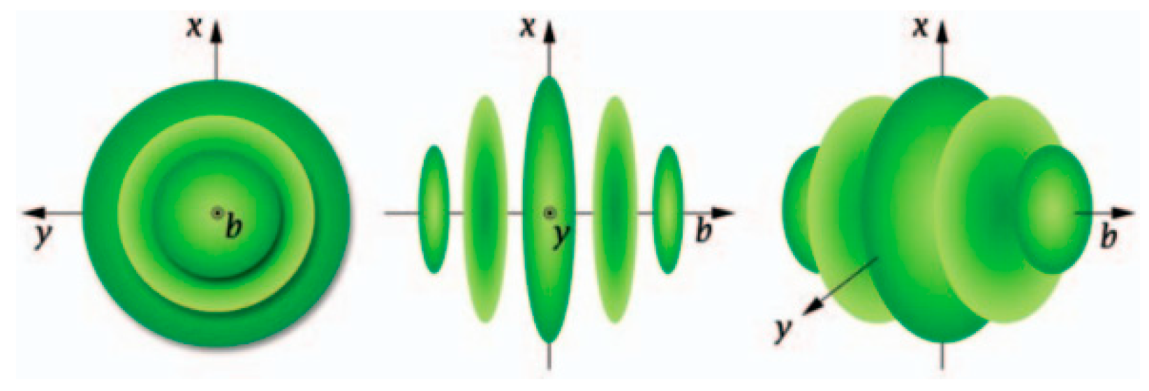
In recent years, many researchers have introduced wavelet decomposition into hyperspectral classification tasks and proposed many novel classification methods [27,28,29,30]. For example, in 3DGPC-HDM framework [28], a three-dimensional Gabor wavelet (Figure 1) was introduced to extract the joint spectral-spatial features of HSI, and a phase coding and Hamming-distance matching framework based on the three-dimensional Gabor wavelet was proposed. Cao etc. 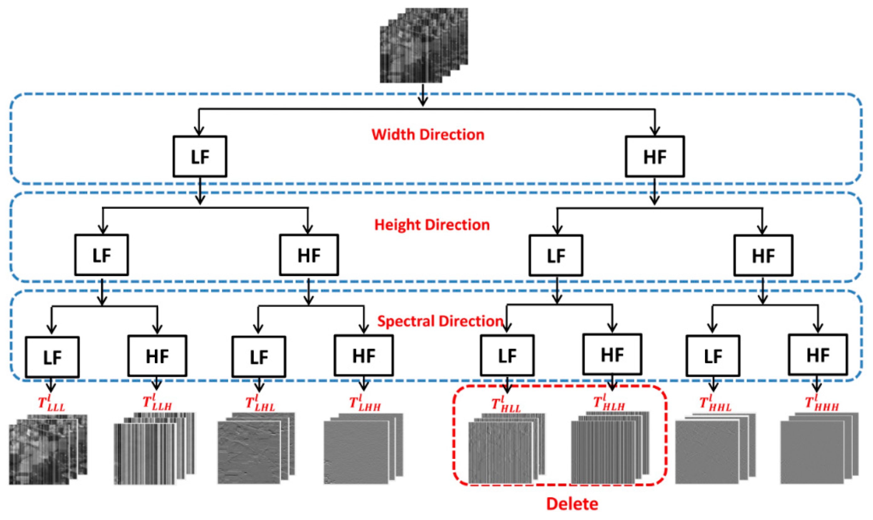[30] proposed an enhanced 3DDWT (E-3DDWT, Figure 2) method which discarded partial of the sub cubes after wavelet decomposition to extract features and alleviate the noise simultaneously. 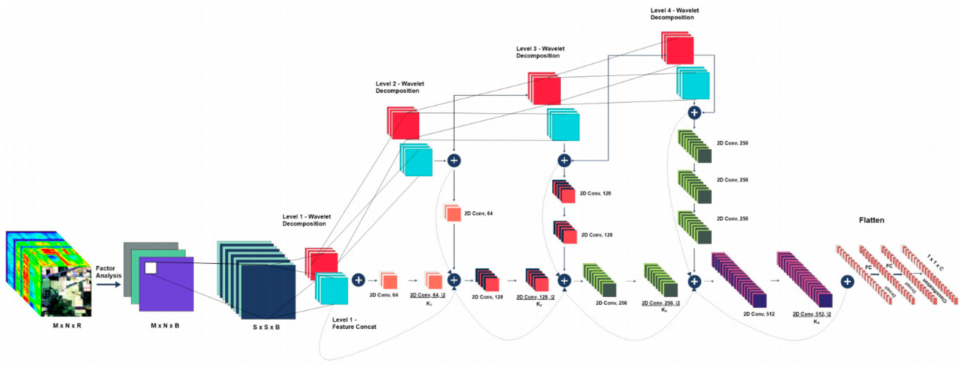SpectralNet [31] carried out four-layer wavelet decomposition of HSI blocks, extracted further features by CNN and then classified (Figure 3). It had achieved very good results on the three classical HSI datasets, however, the number of parameters in the model was relatively large, about 6-7M.

However, there are two problems for most of the above wavelet-based models. One is the heavy training parameters and the other is that there is no distinction between the classification effectiveness of low frequency and high frequency features after wavelet decomposition, both low and high frequency components are used in the classification model.

In this paper, a light-weighted low frequency wavelet-based convolutional neural network model LLFWCNN is proposed. There are two main contributions of this paper:

The proposed LLFWCNN using a combination of wavelet decomposition, feature reshape and a well-designed CNN to obtains comparable or even better results and fewer parameters than other state-of-the-art models, especially in small samples.
It proves that the influence of low frequency and high frequency after wavelet decomposition on HSIC is different. The low frequency features include much more advantageous information for HSIC than high frequency features. Low frequency component is enough.

2. Proposed Model

2.1. Overall Architecture

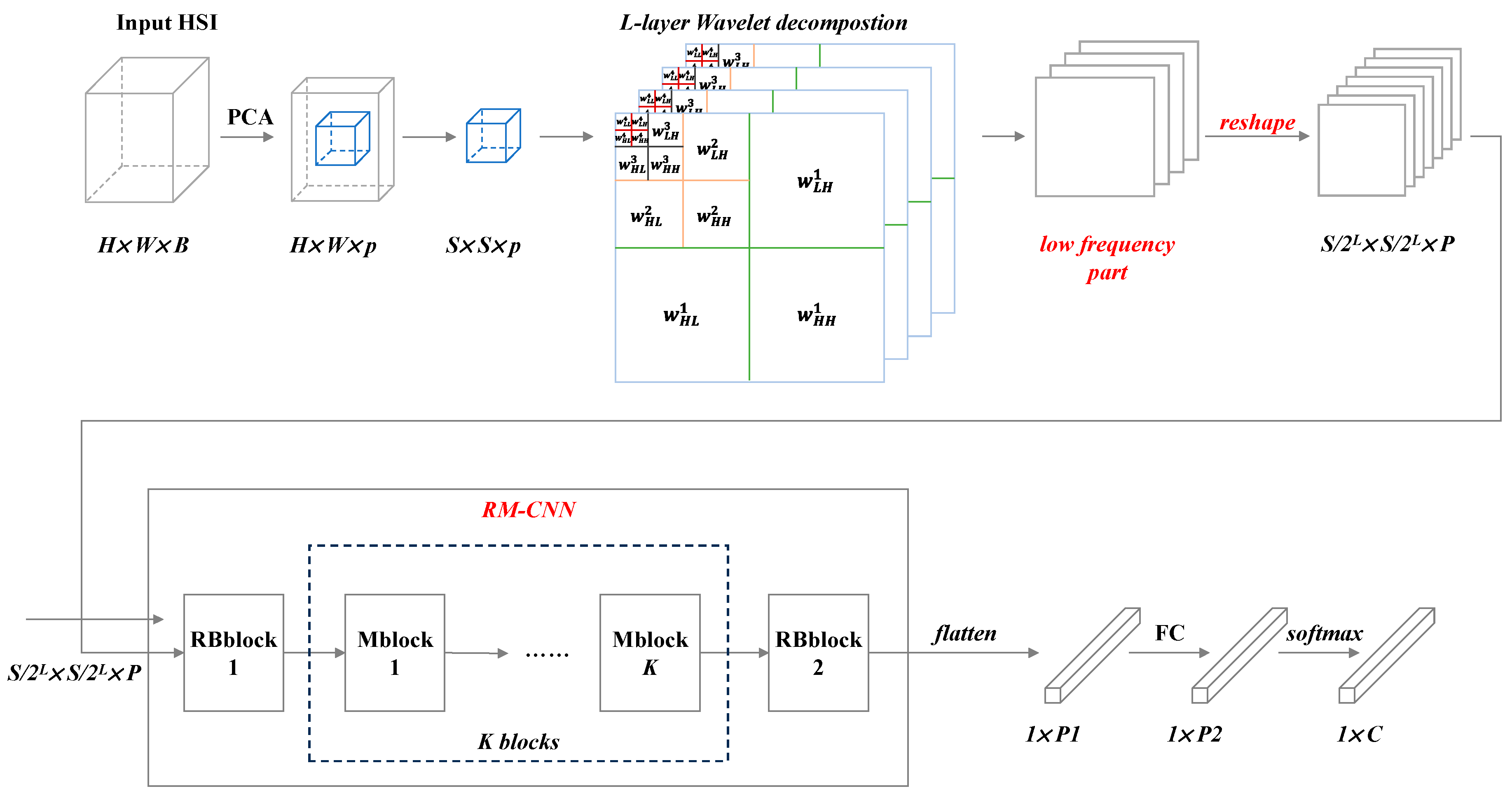
The overall architecture of LLFWCNN is shown as Figure 4.

The LLFWCNN contains the following four stages: dimension reduction, wavelet decomposition, feature extraction and classification, the first three of which are described in detail below.

2.2. Dimension Reduction and Wavelet Decomposition

2.2.1. Dimension Reduction

In order to effectively reduce the computational complexity of HSI data, we introduce Principal Component Analysis (PCA) method as preprocessing to lower the dimensionality of the original HSI. PCA is one of the most widely used data dimensionality reduction algorithms, which preserve the most important features of the original high dimensional data and map the high dimensional data to the low dimensional space.

The original input HSI is

X_{i m a g e} \in R^{H \times W \times B}

，where H, W and B represent the length, width and spectral dimension of HSI respectively. After PCA dimension reduction, the input X_image is transformed to

X_{i m a g e}^{'} \in R^{H \times W \times p}

(p<<B).

2.2.2. Wavelet Decomposition

Wavelet decomposition is carried out on the resized HSI. Wavelet decomposition is a classical method for signal processing and analysis. Figure 5 illustrates the process of how two-dimensional discrete wavelet decomposition works on images.

The image is decomposed into four sub-bands by two-dimensional wavelet decomposition, in which the LL sub-band is the low frequency component, and the HL, LH and HH sub-bands are the high frequency components in the horizontal, vertical and diagonal directions, respectively. The low frequency component with a low resolution is an approximation to the original image and describes the main part of the image. While the high frequency component embodies the details of the image.

The procedure after dimension reduction is divided into three steps as follow:

1) Firstly, extract the hyperspectral input cube

X_{c u b e}^{0} \in R^{S \times S \times p}

pixel by pixel from the pre-processed input HSI

X_{i m a g e}^{'}

, where S represents the cube size.

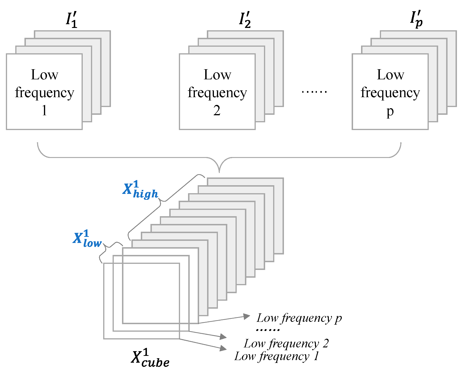
2) Secondly, a two-dimensional wavelet decomposition is performed on a single image

I_{m} \in R^{S \times S \times 1}

（m=1, 2, …, p）extracted from

X_{c u b e}^{0}

along the spectral dimension, forming the result denoted as

I_{m}^{'}

（m=1, 2, …, p）with the size

S / 2 \times S / 2 \times 4

. p images from p bands lead to p features

I_{m}^{'}

（m=1, 2, …, p）.

3) Thirdly, the p features

I_{m}^{'}

（m=1, 2, …, p）are stacked in the order of "low frequency + high frequency", and then obtain the wavelet decomposition result

X_{c u b e}^{1} \in R^{S / 2 \times S / 2 \times 4 p}

(Figure 6). The low frequency part of

X_{c u b e}^{1}

is denoted as

X_{l o w}^{1}

, and the high frequency part is denoted as

X_{h i g h}^{1}

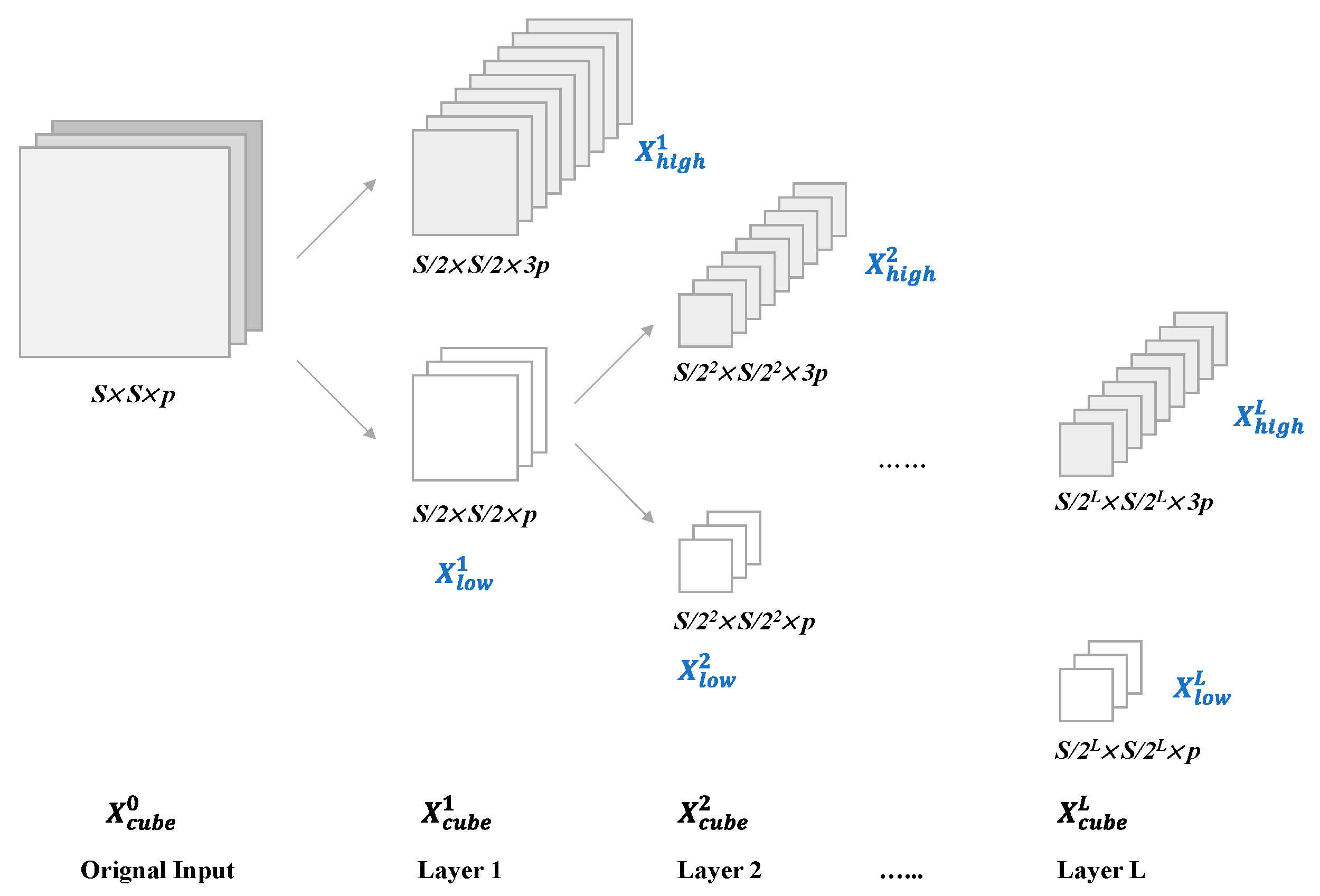
4) The low frequency part

X_{l o w}^{1}

is selected and decomposed until the Lth layer in the above way to get the result

X_{c u b e}^{L} \in R^{S / 2^{L} \times S / 2^{L} \times 4 p}

of the L-layer wavelet decomposition. The complete procedure is shown in Figure 7.

2.2.3. Feature Reshape

Feature reshape is a very important step in the LLFWCNN. Except the results obtained in the last wavelet decomposition layer, the results of each layer were reshaped to the size of the features of the last layer.

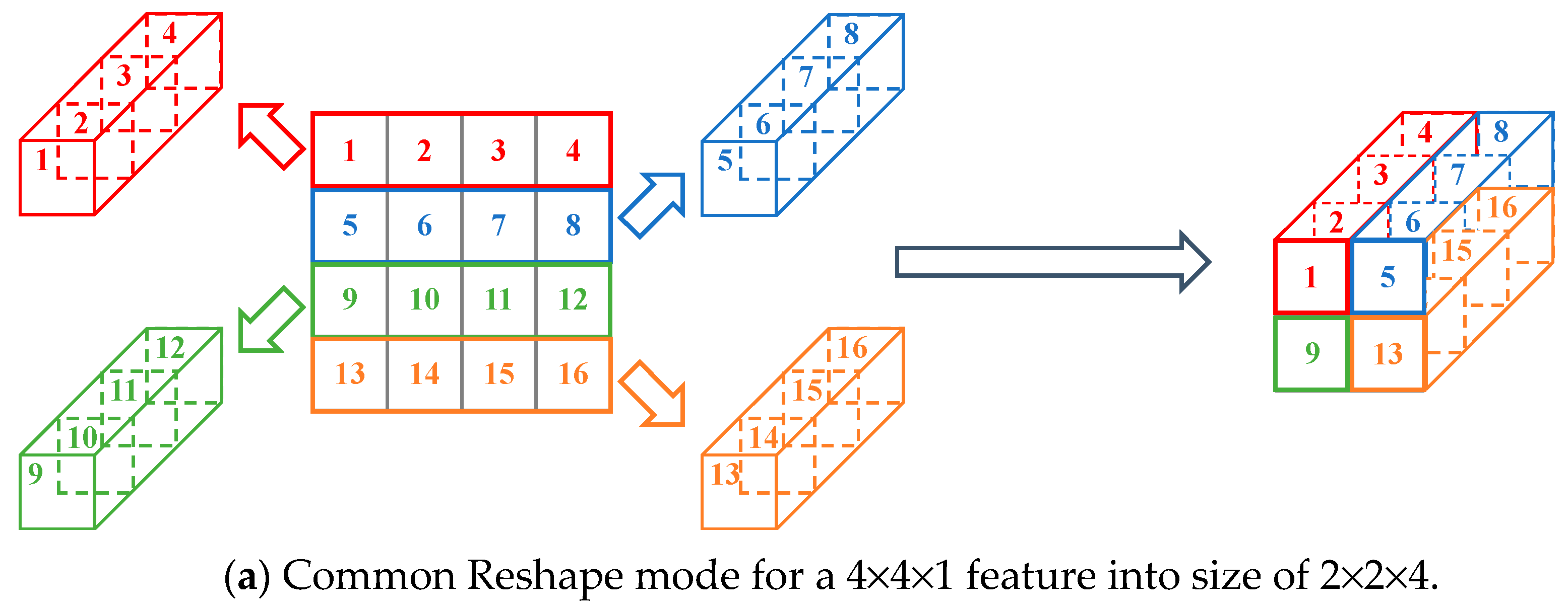
The commonly used reshape mode for a single image is “reshape by row”. For example, if we want to reshape a 4×4×1 feature into size of 2×2×4, the reshape mode is shown in Figure 8(a). In this mode, each row vector of size 1×4×1 is rearranged to a vector of size 1×1×4 (left part of Figure 8(a)). And then the four new vectors were stacked in the order (right part of Figure 8(a)) to obtain the feature cube of size 2×2×4.

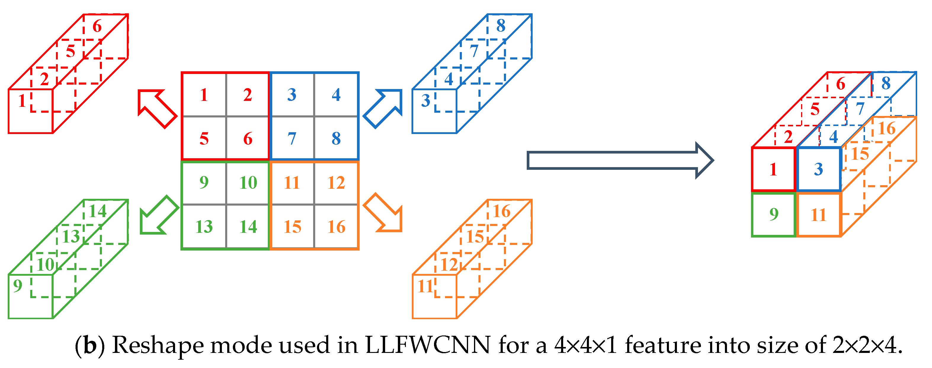
However, this mode is not suitable when the feature is a result of wavelet decomposition. Because there is inner relationship among the pixels in a square area not in a row. Therefore, another reshape mode was used. For the above example, pixels in a specific 2×2 square area are considered to be intrinsically related. Figure 8(b) shows how the reshaping is executed.

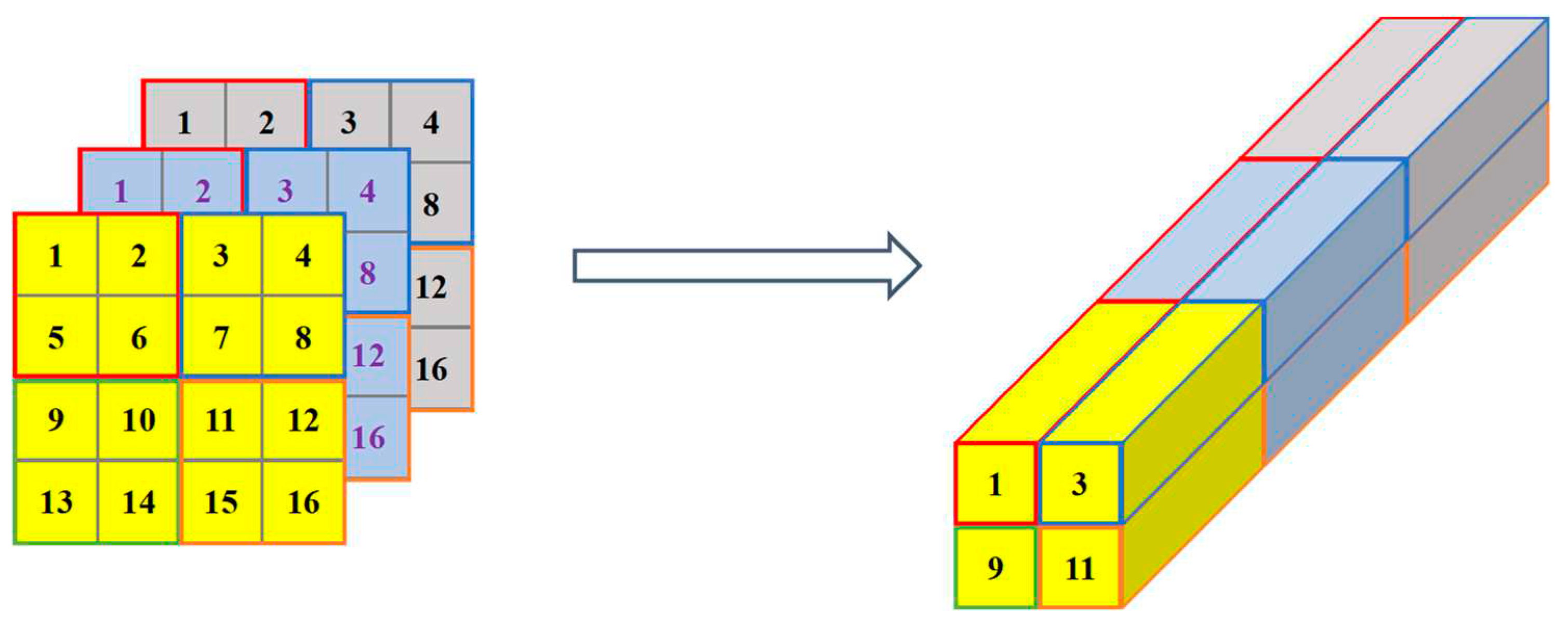
After the features of multi-channels were reshaped, they were stacked in the way as in Figure 9. Hence, in this stage, each

X_{c u b e}^{i} \in R^{S / 2^{i} \times S / 2^{i} \times 4 p}

(i≠L) was finally reshaped to

X_{c u b e}^{i'} \in R^{S / 2^{L} \times S / 2^{L} \times 4^{L - i} \times p}

, that helps to reduce the parameters in the next CNN stage.

2.3. Convolutional Neural Network RM-CNN

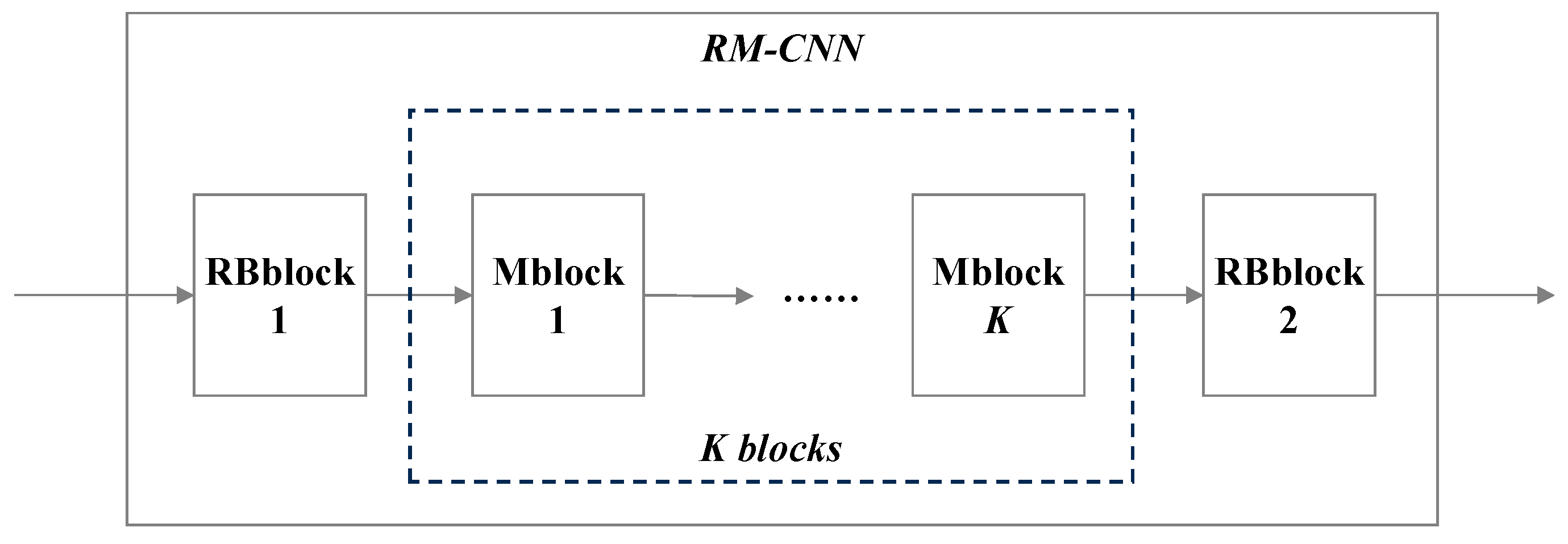
Following the wavelet decomposition, there is a specially designed convolutional neural network RM-CNN. The detailed structure is shown in Figure 10.

RM-CNN consists of two different types of modules: Rblock and Mblock. There is one Rblock at the front and end of the network each. It mainly realizes feature extraction and pooling. The spatial size of the output feature is reduced to half of the original input feature when passing through Rblock. Compared with Rblock, Mblock does not have a pooling layer, but adopts skip connection. It brings two benefits, one of which is to maintain the spatial size of the output feature and the other is to keep the original input feature information from being lost by adding input information. K is a hyper-parameter denoting the number of Mblock. The inner structures of Rblock and Mblock are shown in Figure 11(a) and (b).

In Figure 11(a), n is the number of convolutional kernels in convolutional layer. It can be the same or not the same as b in Rblock, while in Mblock it must be the same as b.

Through the combined use of Reshape and RM-CNN, we achieved the goal of reducing the number of parameters. Because the spatial size of the last features after wavelet decomposition is relatively small, and was designed to be 4×4 or 6×6. After spatial dimension reduction twice by RMCNN, the output size could be restricted to 1×1 or 2×2, so that the number of parameters in the fully connected layer would be effectively reduced. For example, there is a feature cube of size 16×16×12. The number of convolutional kernels in Rblock and Mblock are 32, and kernel size is 3×3.

The parameter differences between reshaping and non-reshaping are listed in Table 1, and the parts with the same parameters are omitted.

It is clear that the number of parameters after reshaping is only one-tenth of that without reshaping.

3. Experiment

3.1. Datasets

We did experiments on three classical experimental datasets: Indian Pines, Pavia University and Salinas. Indian Pines and Salinas were acquired by the Airborne Visible Infrared Imaging Spectrometer (AVIRIS) sensor over the Indian Pines test site in North-western Indiana and Salinas Valley. And Pavia University was captured by the Reflective Optics System Imaging Spectrometer (ROSIS-03). AVIRIS provides 224 contiguous spectral bands, covering wavelengths from 0.4 to 2.5μm and with a spatial resolution of 20m/pixel, while ROSIS-03 delivers 115 bands with a spectral coverage ranging from 0.43 to 0.86μm and with a spatial resolution of 1.3m/pixel. And we used a corrected version of them by removing some water absorption bands and a blank strip. Indian Pines consists 145×145 pixels, Salinas consists 512×217 pixels and Paiva University consists of 610×340 pixels. Both Indian Pines and Salinas consist of 16 ground-truth classes while Pavia University contains 9 different classes.

3.2. Settings

3.2.1. Hyper-parameter Settings

There are six hyper-parameters of LLFWCNN, which are input spatial size, PCA value, depth of wavelet decomposition, number of Rblock and Mblock and nodes in fully connected layer. Different configurations for different datasets are listed in Table 2.

3.2.2. Training parameter Settings

Parameters related to training are shown in Table 3. The stochastic gradient descent (SGD) method was chosen for optimization. Batch size and learning rate were the same for all datasets that were 8 and 0.02, but the epoch was different. Training proportion was set to 10% and 30% to illustrate performance of all the six compared models. Table 4, Table 5 and Table 6 give the detailed split of training and testing on the three datasets.

The running environment is: CPU i7-10700, GPU Nvidia GeForce RTX 2070, 8G video memory.

3.3. Results and Analysis of the Experiment

Experiments on each dataset were carried out 5 to 10 times to ensure the accuracy and reliability. Three commonly used measurement indicators: Overall Accuracy (OA), Average Accuracy (AA) and Kappa Coefficient (Kappa) were adopted. And their corresponding data listed in all the following tables are multiplied by 100.

3.3.1. Comparisons of classification results

We compared the classification results of LLFWCNN and SpectralNet [31], 2D CNN [32], 3D CNN [32], M3D CNN [33], FuSENET [34].

Table 7 and Table 8 list the results under proportion 1 and 2. Optimal results are shown in bold, and sub-optimal results are shown in italics.

From the data of Table 2 and Table 3 we found that both LLFWCNN and SpectralNet can perform well, outperforming other models. Then, we further reduced the proportion of training samples to 5% and 1% to evaluate the classification effects of the two models under even smaller samples. The results are given in Table 9.

3.3.2. Comparison of the parameters

We compared the number of parameters of LLFWCNN with that of SpectralNet. And the results are shown in Table 10.

Based on the data in Table 7, Table 8, Table 9 and Table 10, it can be seen that with only about 1/40 of the parameters of SpectralNet, LLFWCNN obtains the same classification results as SpectralNet, and even better classification results under small sample (training sample proportion 5%, 1%).

3.3.3. Ablation experiment

Ablation experiments were done to evaluate the performance of the low frequency component and high frequency component. In the next tables,

X_{l o w}^{i}

represented using only low frequency,

X_{h i g h}^{i}

represented using only high frequency and

X_{l o w}^{i} {+ X}_{h i g h}^{i}

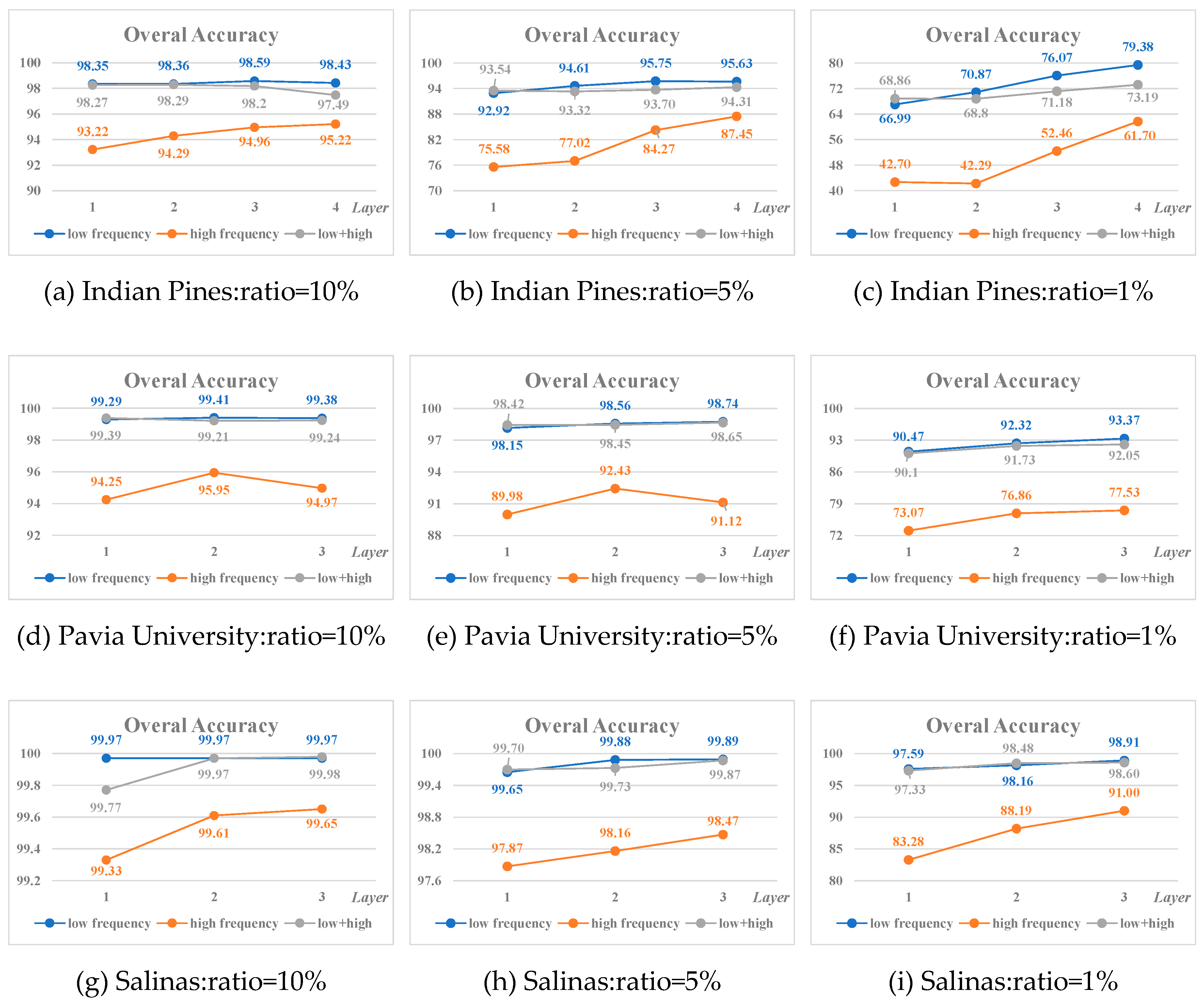
represented using both. The training sample proportions were set to 10%, 5%, and 1% for all the three datasets. The classification indicators of the three datasets were shown in Table 11, Table 12, Table 13, Table 14, Table 15, Table 16, Table 17, Table 18 and Table 19. And Figure 11(a)-(i) show the variation of the overall accuracy at the ratio of 10%, 5% and 1%, respectively.

Figure 11. Variation of the Overall Accuracy on the three datasets.

As can be seen from the experiment results in Table 11, Table 12, Table 13, Table 14, Table 15, Table 16, Table 17, Table 18 and Table 19 and Figure 11, the effects of low frequency and high frequency components after wavelet decomposition on HSIC are indeed significantly different.

1) The classification result of low frequency features is better or much better than that of high frequency features;

2) For datasets itself with large sample such as Pavia University and Salinas, the smaller the proportion of training samples, the better the effect of using low frequency component

X_{l o w}^{i}

for classification. While for dataset with a small sample e.g. Indian Pines, the advantage of using low frequency component

X_{l o w}^{i}

for classification is more obvious;

3) For the different components from the same layer after wavelet decomposition, the classification effect of the mixed features of low frequency and high frequency is between that of the low frequency and high frequency;

4) In most cases, the higher the decomposition level, the better the classification results of the corresponding low frequency or high frequency features, especially when the sample size is small (such as 1%). The best classification results of the three datasets are obtained by the low frequency component at the highest wavelet decomposition level.

3.3.4. Parameters of different frequency

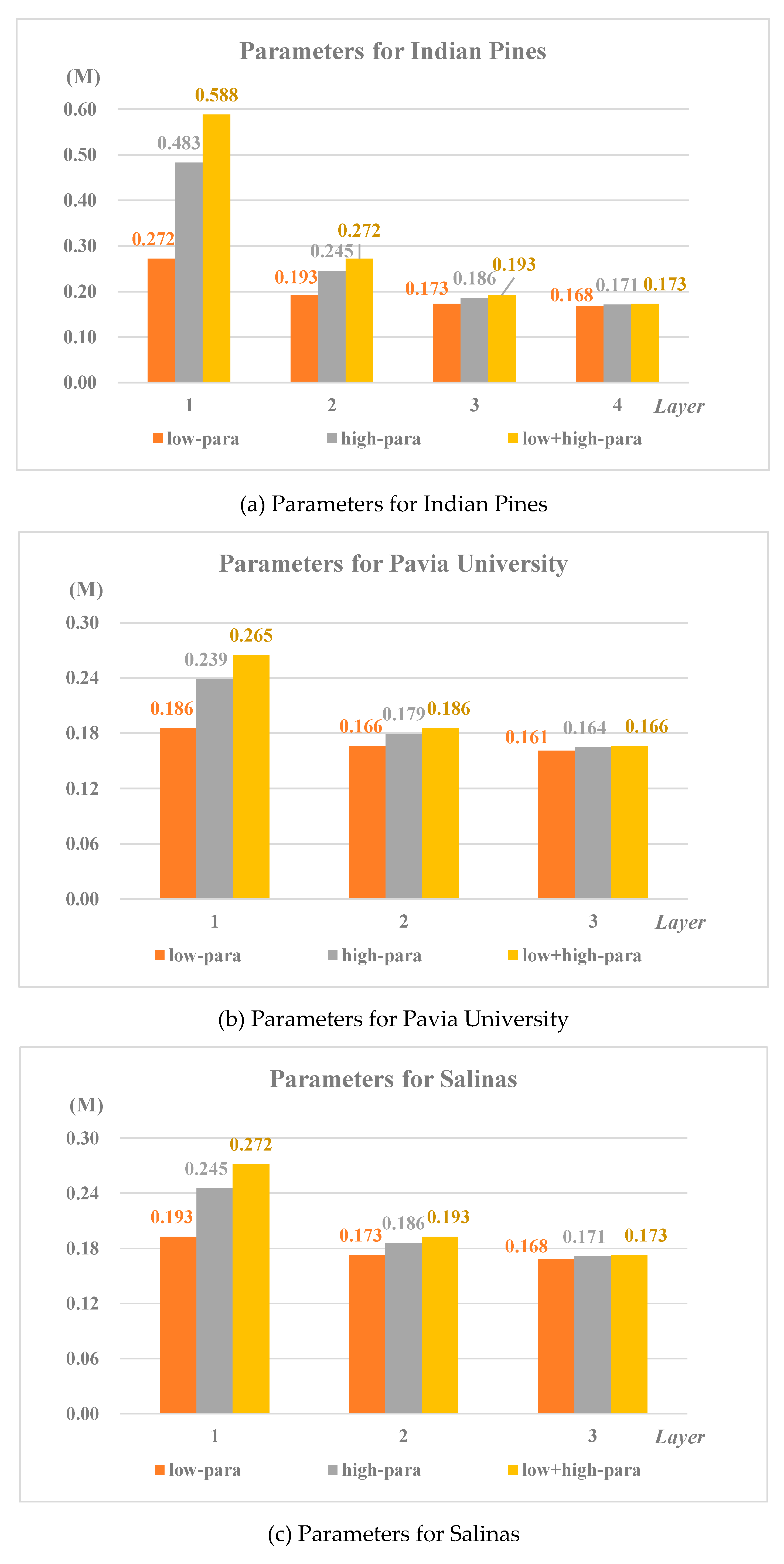
At the same time, a comparison of the number of parameters used in the classification for low frequency and high frequency of different layers is shown in Figure 12(a)-(c).

Two conclusions can be drawn from Figure 12:

1) When using the features of different layers to classify, the number of parameters producing in the model is different. The deeper the layer number, the smaller the number of parameters;

2) When low frequency component and high frequency component participate in classification, the number of parameters producing in the model is also different, which is smaller for low frequency than that of high frequency.

3.3.5. Influence of other hyper-parameters

In paragraph 3.2, we listed the settings for most of the hyper-parameters. In fact, during the experiments, the best value of the hyper-parameters was not easy to determine. Most of the time, we took all aspects of the factors in consideration, and finally determined a most appropriate value.

For example, considering the requirement of wavelet decomposition, the input spatial size was first set to 16, 32, 64 which were multiples of 2. And then some available values were also tried, e.g. 24, 48. At the same time, the bigger the input size, the bigger the depth of the wavelet decomposition. Otherwise, the input for RMCNN would be bigger and produce more parameters.

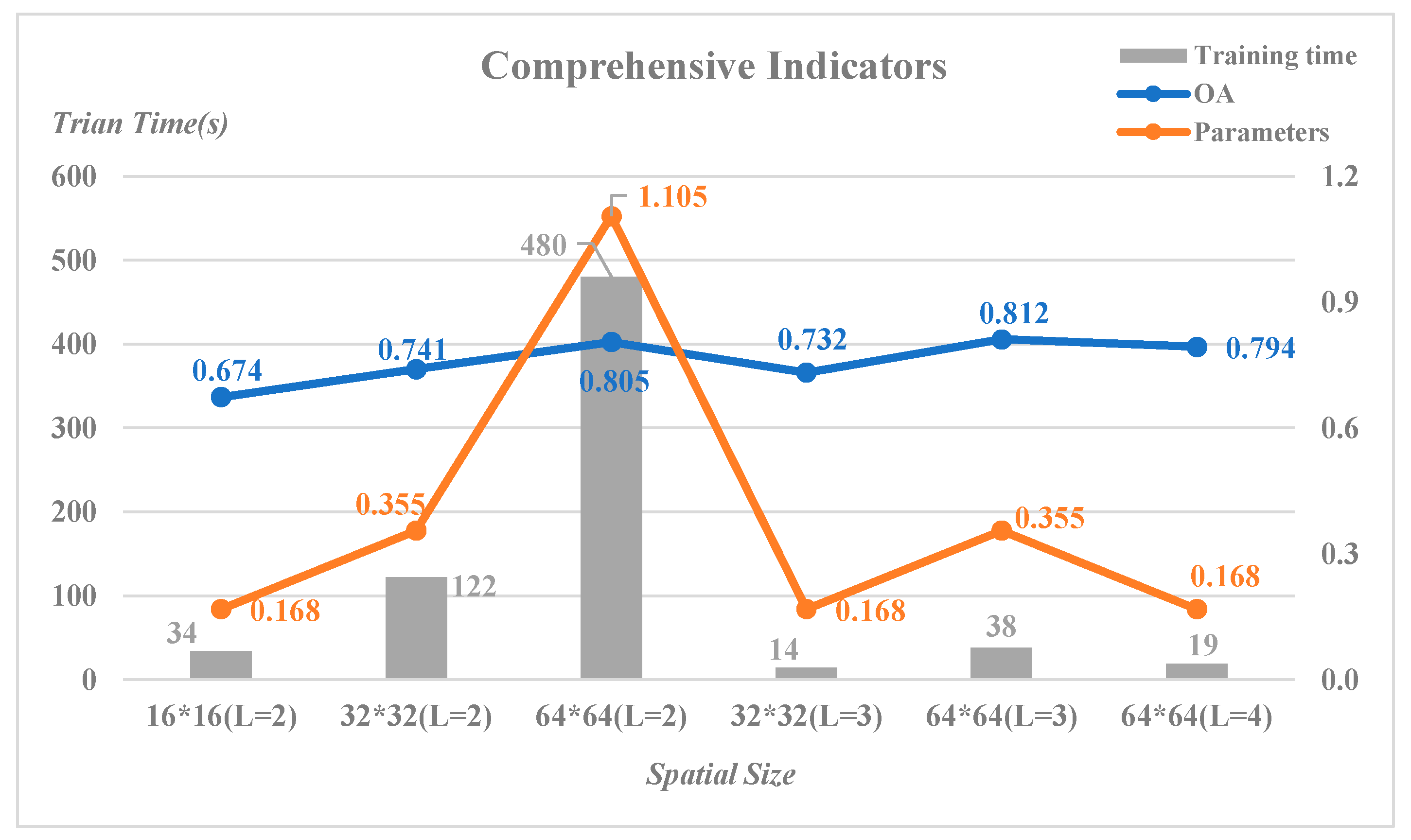
Take Indian Pines for example. The low frequency features after the last wavelet decomposition were feed to the model and training ratio was 1%. Figure 13 is a comprehensive illustration for all the influential factors to be taken into account of.

At the same level (L=2) of wavelet decomposition, the overall accuracy raised when it turned from 16 to 64. And the number of parameters and training time increased as well. The increase of OA was relatively small, but the increase of parameter number and training time were very large. A similar situation occurred when it came to a high level (L=3). Because of the small size of Indian Pines itself, the larger input such as 128×128 was not used.

We could see that the three optimal OA results were the results of the same input 64×64 when L was 2, 3, 4 respectively. When the number of parameters, the training time and the training ratio were all taken into account, setting the depth of wavelet decomposition be 4 was better.

For Pavia University and Salinas, the same experiments were carried out, and the final hyper-parameters were set as shown in Table 2.

4. Conclusion

In this paper, a LLFWCNN network model is proposed to classify HSI after two-dimensional wavelet decomposition. The following conclusions can be drawn from results of the experiments:

1. LLFWCNN uses fewer parameters to obtain a comparable classification effect compared with other excellent models, especially in the case of small samples.

2. Results of the experiment show that spatial information from the low frequency and high frequency after wavelet decomposition have different effects on HSIC. Spatial information of the low frequency contains more favorable information for classification, which is relatively more useful.

3. The classification results of the LLFWCNN model prove that the low frequency features after wavelet decomposition already have enough effective information. It can be considered to discard the high frequency components after wavelet decomposition or to employ different processing methods to improve the efficiency of the use of high frequency components in terms of the different effects of the low frequency and high frequency components on HSIC.

The conclusions above provide effective experimental support for the follow up study on how to make full use of wavelet decomposition in HSIC in the case of small samples.

Author Contributions

All the authors contribute significantly to the research. Methodology, Linlin Chen and Zhihui Wei; Software, Linlin Chen and Huiming Shuai; Writing – original draft, Linlin Chen; Writing – review & editing, Linlin Chen, Zhihui Wei and Yang Xu.

Acknowledgments

This work was supported in part by the National Natural Science Foundation of China under Grant U23B2006,92370203, 62071233，in part by the Jiangsu Provincial Innovation Support Program under Grant BZ2023046, in part by the Jiangsu Provincial Natural Science Foundation of China under and Grant BK20170858, BK20211570, in part by the Jiangsu Provincial Key Research and Development Program under Grant BE2022065-2.

Conflicts of Interest

The authors declare no conflict of interest.

References

Noor, S.; Michael, K.; Marshall, S.; Ren, J.; Tschannerl, J.; Kao, F. The properties of the cornea based on hyperspectral imaging: Optical biomedical engineering perspective. In Proceedings of the International Conference on Systems, Signals and Image Processing (IWSSIP), Bratislava, Slovakia, 23-25 May 2016; pp. 1–4. [Google Scholar]
Wang, J.; Zhang, L.; Tong, Q.; Sun, X. The spectral crust project—Research on new mineral exploration technology. In Proceedings of the 4th IEEE GRSS Workshop on Hyperspectral Image and Signal Processing: evolution in remote sensing (WHISPERS), Shanghai, China, 4-7 June 2012; pp. 1–4. [Google Scholar]
Ardouin, J.-P.; Lévesque, J.; Rea, T. A demonstration of hyperspectral image exploitation for military applications. In Proceedings of the 10th International Conference on Information Fusion, Quebec, QC, Canada, 9-12 July 2007; pp. 1–8. [Google Scholar]
Liang, L.; Di, L.; Zhang, L.; Deng, M.; Qin, Z.; Zhao, S.; Lin, H. Estimation of crop LAI using hyperspectral vegetation indices and a hybrid inversion method. Remote Sens. Environ. 2015, 165, 123–134. [Google Scholar] [CrossRef]
Tidke, S.; Kumar, A. New HyperSpectral Image Segmentation based on the Concept of Binary Partition Tree. Int. J. Advanced Technology and Engineering Exploration. 2015, 2, 140–146. [Google Scholar]
Lu, X.; Li, X.; Mou, L. Semi-supervised multitask learning for scene recognition. IEEE Trans. Cybern. 2015, 45, 1967–1976. [Google Scholar]
Hecker, C.; Meijde, M.; Werff, H.; Meer, F. Assessing the influence of reference spectra on synthetic SAM classification results. IEEE Trans. Geosci. Remote Sens. 2008, 46, 4162–4172. [Google Scholar] [CrossRef]
Demir, B.; Erturk, S. Hyperspectral Image Classification Using Relevance Vector Machines. IEEE Geosci. Remote Sens. Lett. 2007, 4, 586–590. [Google Scholar] [CrossRef]
Camps-Valls, G.; Gómez-Chova, L.; Muñoz, J.; Vila-Francés, J.; Calpe, J. Composite kernels for hyperspectral image classification. IEEE Geosci. Remote Sens. Lett. 2006, 3, 93–97. [Google Scholar] [CrossRef]
Licciardi, G.; Marpu, P.; Chanussot, J.; Benediktsson, J. Linear versus nonlinear PCA for the classification of hyperspectral data based on the extended morphological profiles. IEEE Geosci. Remote Sens. Lett. 2012, 9, 447–451. [Google Scholar] [CrossRef]
Li, W.; Chen, C.; Su, H.; Du, Q. Local Binary Patterns and Extreme Learning Machine for Hyperspectral Imagery Classification. IEEE Trans. Geosci. Remote Sens. 2015, 53, 3681–3693. [Google Scholar] [CrossRef]
Li, W.; Wu, G.; Zhang, F.; Du, Q. Hyperspectral Image Classification Using Deep Pixel-Pair Features. IEEE Trans. Geosci. Remote Sens. 2017, 55, 844–853. [Google Scholar] [CrossRef]
Chen, Y.; Jiang, H.; Li, C.; Jia, X.; Ghamisi, P. Deep Feature Extraction and Classification of Hyperspectral Images Based on Convolutional Neural Networks. IEEE Trans. Geosci. Remote Sens. 2016, 54, 6232–6251. [Google Scholar] [CrossRef]
Liang, J.; Zhou, J.; Qian, Y.; Wen, L.; Bai, X.; Gao, Y. On the Sampling Strategy for valuation of Spectral-Spatial Methods in Hyperspectral Image Classification. IEEE Trans. Geosci. Remote Sens. 2017, 55, 862–879. [Google Scholar] [CrossRef]
Cheng, G.; Li, Z.; Han, J.; Yao, X.; Guo, L. Exploring Hierarchical Convolutional Features for Hyperspectral Image Classification. IEEE Trans. Geosci. Remote Sens. 2018, 56, 6712–6722. [Google Scholar] [CrossRef]
Hu, W.; Huang, Y.; Li, W.; Zhang, F.; Li, H. Deep convolutional neural networks for hyperspectral image classification. J. Sensors. 2015, 2015, 1–12. [Google Scholar] [CrossRef]
Yue, J.; Zhao, W.; Mao, S.; Liu, H. Spectral-spatial classification of hyperspectral images using deep convolutional neural networks. Remote Sens. Lett. 2015, 6, 468–477. [Google Scholar] [CrossRef]
Haut, J.; Paoletti, M.; Plaza, J.; Li, J.; Plaza, A. Active Learning with Convolutional Neural Networks for Hyperspectral Image Classification Using a New Bayesian Approach. IEEE Trans. Geosci. Remote Sens. 2018, 56, 6440–6461. [Google Scholar] [CrossRef]
Liang, H.; Li, Q. Hyperspectral imagery classification using sparse representations of convolutional neural network features. Remote Sens. 2016, 8, 99–114. [Google Scholar] [CrossRef]
Makantasis, K.; Protopapadakis, E.; Doulamis, A.; Doulamis, N.; Loupos, C. Deep Convolutional Neural Networks for Efficient Vision Based Tunnel Inspection. In Proceeding of the IEEE International Conference on Intelligent Computer Communication and Processing (ICCP), Cluj-Napoca, Romania, 3-5 September 2015; pp. 335–342. [Google Scholar]
Li, Y.; Zhang, H.; Shen, Q. Spectral-Spatial Classification of Hyperspectral Imagery with 3D Convolutional Neural Network. Remote Sens. 2017, 9, 67–87. [Google Scholar] [CrossRef]
Zhong, Z.; Li, J.; Luo, Z.; Chapman, M. Spectral-Spatial Residual Network for Hyperspectral Image Classification: A 3-D Deep Learning Framework. IEEE Trans. Geosci. Remote Sens. 2018, 56, 8457–858. [Google Scholar] [CrossRef]
Paoletti, M.; Haut, J.; Plaza, J.; Plaza, A. A New Deep Convolutional Neural Network for Fast Hyperspectral Image Classification. ISPRS J. Photogramm. Remote Sens. 2018, 145, 120–147. [Google Scholar] [CrossRef]
Yang, J.; Zhao, Y.; Chan, J. Learning and Transferring Deep Joint Spectral-Spatial Features for Hyperspectral Classification. IEEE Trans. Geosci. Remote Sens. 2017, 55, 4729–4742. [Google Scholar] [CrossRef]
Zhang, H.; Li, Y.; Zhang, Y.; Shen, Q. Spectral-spatial classification of hyperspectral imagery using a dual-channel convolutional neural network. Remote Sens. Lett. 2017, 8, 438–447. [Google Scholar] [CrossRef]
Roy, S.; Krishna, G.; Dubey, S.; Chaudhuri, B. HybridSN: Exploring 3D-2D CNN Feature Hierarchy for Hyperspectral Image Classification. IEEE Geosci. Remote Sens. Lett. 2020, 17, 277–281. [Google Scholar] [CrossRef]
Jia, S.; Zhang, M.; Zhu, J. Gabor Wavelet Based Feature Extraction and Fusion for Hyperspectral and Lidar Remote Sensing Data. In Proceedings of the IEEE International Geoscience and Remote Sensing Symposium (IGARSS), Valencia, Spain, 22-27 July 2018; pp. 1–4. [Google Scholar]
Jia, S.; Shen, L.; Zhu, J.; Li, Q. A 3-D Gabor Phase-Based Coding and Matching Framework for Hyperspectral Imagery Classification. IEEE Trans. Cybern., 2018, 48, 1176–1188. [Google Scholar]
Xiao, G.; Wang, X.; Liu, D. Wavelet transformation of functional data for hyperspectral image classification. In Proceedings of the 2019 International Conference on Internet of Things (iThings) and IEEE Green Computing and Communications (GreenCom) and IEEE Cyber, Physical and Social Computing (CPSCom) and IEEE Smart Data (SmartData), Atlanta, GA, USA, 14-17 July 2019; pp. 403–409. [Google Scholar]
Cao, X.; Yao, J.; Fu, X.; Bi, H.; Hong, D. An Enhanced 3-D Discrete Wavelet Transform for Hyperspectral Image Classification. IEEE Geosci. Remote Sens. Lett. 2021, 18, 1104–1108. [Google Scholar] [CrossRef]
Tanmay, C.; Utkarsh, T. SpectralNET: Exploring Spatial-Spectral WaveletCNN for Hyperspectral Image Classification. arXiv, 2021; arXiv:2104.00341v1. [Google Scholar]
Yang, X.; Ye, Y.; Li, X.; Raymond, Y. K. Lau; Zhang, X.; Huang, X. Hyperspectral image classification with deep learning models. IEEE Trans. Geosci. Remote Sens. 2018, 56, 5408–5423. [Google Scholar] [CrossRef]
He, M.; Li, B.; Chen, H. Multi-scale 3d deep convolutional neural network for hyperspectral image classification. In Proceedings of the 2017 IEEE International Conference on Image Processing (ICIP), Beijing, China, 17-20 September 2017; pp. 3904–3908. [Google Scholar]
Roy, S. K. FuSEnet: fused squeeze-and-excitation network for spectral-spatial hyperspectral image classification. IET Image Processing 2020, 14, 1653–1661. [Google Scholar] [CrossRef]

Figure 1. Three-dimensional Gabor wavelet [28].

Figure 2. Lth level decomposition procedure of E-3DDWT [30].

Figure 3. Architecture of SpectralNet [31].

Figure 4. The overall architecture of LLFWCNN.

Figure 5. Process of two-dimensional discrete wavelet decomposition.

Figure 6. Stack mode for the feature of the ith-layer wavelet decomposition.

Figure 7. Procedure of multilayer wavelet decomposition.

Figure 8. Different Reshape mode.

Figure 9. Stack mode for all

X_{c u b e}^{i} (i \neq L)

Figure 9. Stack mode for all

X_{c u b e}^{i} (i \neq L)

Figure 10. Structure of the RM-CNN.

Figure 11. Structure design of the two kinds of blocks.

Figure 12. Parameters used in the classification for low frequency and high frequency of different layers.

Figure 13. The different influence of input spatial size.

Table 1. Parameter settings of LLFWCNN for different datasets.

Input	Reshape	Output	Para in Rblock1	Output2	FC	Para in FC	Total
16×16×12	Yes	4×4×48	13824	1×1×32	1024	32768	46592
16×16×12	No	16×16×12	864	4×4×32	1024	524288	525152

Table 2. Hyper-parameter settings of LLFWCNN for different datasets.

Datasets	Spatial Size	PCA	L*	Rblock	Mblock	FC
Indian Pines	64×64	3	4	2	2	1024
Pavia University	32×32	3	3	2	2	1024
Salinas	48×48	3	3	2	2	1024

*L is the depth of wavelet decomposition.

Table 3. Training parameter settings of LLFWCNN for different datasets.

Datasets	Batch size	Learning rate	Drop	Epoch	Optimization Method	Training Proportion
Datasets	Batch size	Learning rate	Drop	Epoch	Optimization Method	1		2
Indian Pines	16	0.002	0.4	150	SGD	10%	30%
Pavia University	16	0.002	0.4	50	SGD	10%	30%
Salinas	16	0.002	0.4	50	SGD	10%	30%

Table 4. Training set split on Indian Pines.

(a) training proportion=10%		(b) training proportion=30%
Classes	Train	Test
Alfalfa	5	41
Corn-notill	143	1285
Corn-mintill	83	747
Corn	24	213
Grass-pasture	48	435
Grass-trees	73	657
Grass-pasture-mowed	3	25
Hay-windrowed	48	430
Oats	2	18
Soybean-notill	97	875
Soybean-mintill	245	2210
Soybean-clean	59	534
Wheat	20	185
Woods	126	1139
Buildings-Grass-Trees-Drives	39	347
Ston-Steel-Towers	9	84
Total	1024	9225
Classes	Train	Test
Alfalfa	14	32
Corn-notill	428	1000
Corn-mintill	249	581
Corn	71	166
Grass-pasture	145	338
Grass-trees	219	511
Grass-pasture-mowed	8	20
Hay-windrowed	143	335
Oats	6	14
Soybean-notill	292	680
Soybean-mintill	736	1719
Soybean-clean	178	415
Wheat	62	143
Woods	379	886
Buildings-Grass-Trees-Drives	116	270
Ston-Steel-Towers	28	65
Total	3074	7175

Table 5. Training set split on Pavia University.

(a) training proportion=10%		(b) training proportion=10%
Classes	Train	Test
Asphalt	663	5968
Meadows	1865	16784
Gravel	210	1889
Trees	306	2758
Painted metal sheets	134	1211
Bare-Soil	503	4526
Bitumen	133	1197
Self-Blocking Bricks	368	3314
Shadows	95	852
Total	4277	38499
Classes	Train	Test
Asphalt	1989	4642
Meadows	5594	13055
Gravel	630	1469
Trees	919	2145
Painted metal sheets	403	942
Bare-Soil	1509	3520
Bitumen	399	931
Self-Blocking Bricks	1105	2577
Shadows	284	663
Total	12832	29944

Table 6. Training set split on Salinas.

(a) training proportion=10%		(b) training proportion=10%
Classes	Train	Test
Brocoli_green_weeds_1	201	1808
Brocoli_green_weeds_2	372	3354
Fallow	197	1779
Fallow_rough_plow	139	1255
Fallow_smooth	268	2410
Stubble	396	3563
Celery	358	3221
Grapes_untrained	1127	10144
Soil_vinyard_develop	620	5583
Corn_senesced_green_weeds	328	2950
Lettuce_romaine_4wk	107	961
Lettuce_romaine_5wk	193	1734
Lettuce_romaine_6wk	91	825
Lettuce_romaine_7wk	107	963
Vinyard_untrained	727	6541
Vinyard_vertical_trellis	181	1626
Total	5412	48717
lasses	Train	Test
Brocoli_green_weeds_1	603	1406
Brocoli_green_weeds_2	1118	2608
Fallow	593	1383
Fallow_rough_plow	418	976
Fallow_smooth	803	1875
Stubble	1188	2771
Celery	1074	2505
Grapes_untrained	3381	7890
Soil_vinyard_develop	1861	4342
Corn_senesced_green_weeds	983	2295
Lettuce_romaine_4wk	320	748
Lettuce_romaine_5wk	578	1349
Lettuce_romaine_6wk	275	641
Lettuce_romaine_7wk	321	749
Vinyard_untrained	2180	5088
Vinyard_vertical_trellis	542	1265
Total	16238	37891

Table 7. Results under proportion 1.

Datasets	Indicators	2DCNN*	3DCNN*	M3DCNN*	FuSENet*	SpectralNet*	LLFWCNN
Indian Pines	OA	80.27±1.2	82.62±0.1	81.39±2.6	97.11±0.2	98.76±0.2	98.59±0.2
	AA	68.32±4.1	76.51±0.1	75.22±0.7	97.32±0.2	98.59±0.1	97.82±0.6
	Kappa	78.26±2.1	79.25±0.3	81.20±2.0	97.25±0.2	98.61±0.1	98.39±0.2
Pavia University	OA	96.63±0.2	96.34±0.2	95.95±0.6	97.65±0.3	99.71±0.1	99.50±0.1
	AA	94.84±1.4	97.03±0.6	97.52±1.0	97.68±0.4	99.62±0.1	98.85±0.2
	Kappa	95.53±0.2	94.90±1.2	93.40±0.4	97.69±0.3	99.43±0.2	99.34±0.1
Salinas	OA	96.34±0.3	85.00±0.1	94.20±0.8	99.23±0.1	99.96±0.2	99.97±0.0
	AA	94.36±0.5	89.63±0.2	96.66±0.5	99.16±0.1	99.96±0.1	99.97±0.0
	Kappa	95.93±0.9	83.20±0.7	93.61±0.3	99.97±0.2	99.97±0.2	99.97±0.0

*Classification results of the models with * are based on the data provided in [31].

Table 8. Results under proportion 2.

Datasets	Indicators	2DCNN*	3DCNN*	M3DCNN*	FuSENet*	SpectralNet	LLFWCNN
Indian Pines	OA	88.90±1.3	90.23±0.2	95.67±0.1	99.01±0.2	99.81±0.1	99.70±0.1
	AA	87.01±1.6	89.87±0.1	94.60±0.6	98.64±0.1	99.40±0.5	99.51±0.3
	Kappa	85.70±1.0	89.70±0.3	94.70±0.3	98.60±0.1	99.79±0.1	99.66±0.1
Pavia University	OA	96.50±0.4	97.90±0.3	97.60±0.2	99.42±0.2	99.94±0.1	99.88±0.0
	AA	96.00±0.1	97.30±0.1	98.00±0.1	99.33±0.2	99.97±0.0	99.78±0.0
	Kappa	96.55±0.3	97.22±0.1	96.50±0.6	99.21±0.3	99.92±0.1	99.85±0.0
Salinas	OA	96.75±0.6	95.54±0.5	94.99±0.3	99.68±0.2	99.991±0.0	99.995±0.0
	AA	98.57±0.2	97.09±0.6	96.28±0.2	99.69±0.1	99.992±0.0	99.990±0.0
	Kappa	96.71±0.7	94.81±0.3	95.40±0.1	99.74±0.1	99.990±0.0	99.994±0.0

*Classification results of the models with * are based on the data provided in [31].

Table 9. Classification results of LLFWCNN and SpectralNet under proportion 5% and 1%.

Datasets	Indicators	5%		1%
Datasets	Indicators	SpectralNet	LLFWCNN	SpectralNet	LLFWCNN
Indian Pines	OA	94.38±0.9	95.75±0.4	62.56±2.3	79.38±1.1
	AA	91.08±1.3	91.56±0.9	48.17±2.2	63.52±1.2
	Kappa	93.59±1.0	95.15±0.4	57.55±2.6	76.46±1.3
Pavia University	OA	98.57±0.3	98.66±0.1	79.62±0.9	93.37±0.1
	AA	97.34±0.5	97.28±0.4	67.73±1.5	87.24±0.2
	Kappa	98.11±0.4	98.16±0.3	72.21±1.3	91.15±0.1
Salinas	OA	98.73±1.0	99.89±0.1	82.45±2.1	98.91±0.3
	AA	99.38±0.4	99.88±0.1	85.35±1.1	98.62±0.2
	Kappa	98.59±1.2	99.88±0.1	80.43±2.3	98.79±0.4

Table 10. Parameters of LLFWCNN and SpectralNet.

Datasets	LLFWCNN	SpectralNet	Ratio
Indian Pines	181264≈0.173M	7591504≈7.240M	1:42
Pavia University	168905≈0.161M	6797897≈6.483M	1:40
Salinas	176080≈0.168M	6805072≈6.490M	1:39

Table 11. Classification results of different frequency for Indian Pines (training sample proportion=10%).

Layer	$X_{l o w}^{i}$			$X_{h i g h}^{i}$			$X_{l o w}^{i} {+ X}_{h i g h}^{i}$
Layer	OA	AA	Kappa	OA	AA	Kappa	OA	AA	Kappa
1	98.35±0.2	97.74±0.8	98.12±0.2	93.22±0.6	88.25±2.3	92.27±0.6	98.27±0.2	97.12±0.9	98.03±0.3
2	98.36±0.2	97.78±0.6	98.13±0.3	94.29±0.3	89.89±2.2	93.48±0.3	98.29±0.2	97.48±0.8	98.05±0.3
3	98.59±0.2	97.82±0.6	98.39±0.2	94.96±0.9	91.05±2.2	94.25±1.1	98.20±0.2	96.53±0.9	97.93±0.2
4	98.43±0.1	97.56±0.4	98.21±0.1	95.22±0.5	90.35±0.7	94.55±0.5	97.49±1.1	93.85±1.2	96.91±1.0
All*	OA：98.01±0.2			AA：96.73±0.9			Kappa：97.88±0.2

*All indicates that all the four results (

X_{c u b e}^{i}

, i=12,3,4) of wavelet decomposition (including low frequency and high frequency) are taken as inputs.

Table 12. Classification results of different frequency for Indian Pines (training sample proportion=5%).

Layer	$X_{l o w}^{i}$			$X_{h i g h}^{i}$			$X_{l o w}^{i} {+ X}_{h i g h}^{i}$
Layer	OA	AA	Kappa	OA	AA	Kappa	OA	AA	Kappa
1	92.92±0.6	84.24±0.7	91.92±0.7	75.58±0.6	58.20±1.4	71.94±0.8	93.54±0.4	84.67±2.0	92.61±0.5
2	94.61±0.4	88.85±1.0	93.84±0.4	77.02±0.9	62.25±0.9	73.66±1.0	93.32±0.3	83.34±1.7	92.38±0.3
3	95.75±0.4	91.56±0.9	95.15±0.4	84.27±0.8	69.70±2.5	81.98±0.9	93.70±0.4	84.43±2.1	92.81±0.5
4	95.63±0.2	92.64±1.0	95.01±0.3	87.45±0.2	76.77±1.1	85.58±0.3	94.31±0.4	86.49±3.1	93.50±0.5
All	OA：94.19±0.2			AA：85.53±1.2			Kappa：93.37±0.2

Table 13. Classification results of different frequency for Indian Pines (training sample proportion=1%).

Layer	$X_{l o w}^{i}$			$X_{h i g h}^{i}$			$X_{l o w}^{i} {+ X}_{h i g h}^{i}$
Layer	OA	AA	Kappa	OA	AA	Kappa	OA	AA	Kappa
1	66.99±1.7	49.41±1.2	62.09±1.9	42.70±2.3	25.53±1.5	32.64±3.1	68.86±0.9	49.16±0.7	64.20±1.1
2	70.87±1.7	53.83±1.4	66.65±2.0	42.29±1.4	27.38±1.8	32.97±1.8	68.80±1.6	49.58±1.6	64.16±1.9
3	76.07±1.3	59.63±1.8	72.65±1.5	52.46±1.3	36.30±1.0	44.79±1.4	71.18±1.8	52.63±3.0	66.77±2.1
4	79.38±1.1	63.52±1.2	76.46±1.3	61.70±1.7	43.65±1.6	55.78±2.0	73.19±0.9	53.89±0.8	69.26±1.0
All	OA：69.04±1.0			AA：50.51±1.1			Kappa：64.39±1.1

Table 14. Classification results of different frequency for Pavia University (training sample proportion=10%).

Layer	$X_{l o w}^{i}$			$X_{h i g h}^{i}$			$X_{l o w}^{i} {+ X}_{h i g h}^{i}$
Layer	OA	AA	Kappa	OA	AA	Kappa	OA	AA	Kappa
1	99.29±0.1	98.37±0.2	99.06±0.1	94.25±0.4	90.16±2.0	92.38±0.5	99.39±0.1	98.81±0.2	99.19±0.2
2	99.41±0.1	98.59±0.3	99.22±0.1	95.95±0.3	93.59±2.6	94.63±0.4	99.21±0.2	98.47±0.1	98.96±0.3
3	99.38±0.1	98.42±0.2	99.18±0.1	94.97±0.6	90.23±0.6	93.24±0.8	99.24±0.1	98.29±0.2	99.00±0.1
All*	OA：99.50±0.1			AA：98.85±0.2			Kappa：99.34±0.1

*All indicates that all the three results (

X_{c u b e}^{i}

, i=12,3) of wavelet decomposition (including low frequency and high frequency) are taken as inputs.

Table 15. Classification results of different frequency for Pavia University (training sample proportion=5%).

Layer	$X_{l o w}^{i}$			$X_{h i g h}^{i}$			$X_{l o w}^{i} {+ X}_{h i g h}^{i}$
Layer	OA	AA	Kappa	OA	AA	Kappa	OA	AA	Kappa
1	98.15±0.2	96.49±0.4	97.56±0.3	89.98±1.3	81.33±1.0	86.70±1.8	98.42±0.1	97.10±0.2	97.91±0.2
2	98.56±0.1	97.10±0.2	98.09±0.1	92.43±0.5	85.91±1.3	89.97±0.7	98.45±0.2	96.89±0.4	97.94±0.3
3	98.74±0.1	97.43±0.2	98.33±0.1	91.12±0.8	85.69±0.7	88.21±1.0	98.65±0.1	97.48±0.7	98.21±0.1
All	OA：98.69±0.1			AA：97.38±0.2			Kappa：98.26±0.2

Table 16. Classification results of different frequency for Pavia University (training sample proportion=1%).

Layer	$X_{l o w}^{i}$			$X_{h i g h}^{i}$			$X_{l o w}^{i} {+ X}_{h i g h}^{i}$
Layer	OA	AA	Kappa	OA	AA	Kappa	OA	AA	Kappa
1	90.47±0.3	82.36±0.6	87.23±0.4	73.07±1.1	51.86±1.2	63.43±1.9	90.10±0.5	80.60±0.8	86.73±0.6
2	92.32±0.9	84.75±1.0	89.73±1.1	76.86±1.6	61.28±1.4	68.65±2.5	91.73±0.8	83.32±1.5	88.94±1.1
3	93.37±0.1	87.24±0.2	91.15±0.1	77.53±0.4	64.03±0.6	69.89±0.6	92.05±0.6	84.89±0.6	89.37±0.8
All	OA：91.40±0.4			AA：82.81±0.7			Kappa：88.51±0.6

Table 17. Classification results of different frequency for Salinas (training sample proportion=10%).

Layer	$X_{l o w}^{i}$			$X_{h i g h}^{i}$			$X_{l o w}^{i} {+ X}_{h i g h}^{i}$
Layer	OA	AA	Kappa	OA	AA	Kappa	OA	AA	Kappa
1	99.97±0.0	99.97±0.0	99.97±0.0	99.33±0.2	99.57±0.1	99.25±0.3	99.77±0.4	99.79±0.4	99.74±0.5
2	99.97±0.0	99.97±0.0	99.97±0.0	99.61±0.1	99.74±0.1	99.56±0.1	99.97 ±0.0	99.97±0.0	99.97±0.0
3	99.97±0.0	99.96±0.0	99.96±0.0	99.65±0.1	99.72±0.1	99.61±0.1	99.98 ±0.0	99.97±0.0	99.97±0.0
All	OA：99.97±0.0			AA：99.97±0.0			Kappa：99.97±0.0

Table 18. Classification results of different frequency for Salinas (training sample proportion=5%).

Layer	$X_{l o w}^{i}$			$X_{h i g h}^{i}$			$X_{l o w}^{i} {+ X}_{h i g h}^{i}$
Layer	OA	AA	Kappa	OA	AA	Kappa	OA	AA	Kappa
1	99.65±0.1	99.79±0.0	99.61±0.1	97.87±0.5	98.55±0.6	97.62±0.5	99.70±0.3	99.81±0.1	99.67±0.3
2	99.88±0.0	99.89±0.0	99.87±0.0	98.16±0.4	98.94±0.2	97.95±0.4	99.73±0.3	99.82±0.1	99.70±0.3
3	99.89±0.1	99.88±0.1	99.88±0.1	98.47±0.4	99.03±0.3	98.29±0.5	99.87±0.0	99.88±0.0	99.86±0.0
All	OA：99.84±0.0			AA：99.86±0.1			Kappa：99.82±0.1

Table 19. Classification results of different frequency for Salinas (training sample proportion=1%).

Layer	$X_{l o w}^{i}$			$X_{h i g h}^{i}$			$X_{l o w}^{i} {+ X}_{h i g h}^{i}$
Layer	OA	AA	Kappa	OA	AA	Kappa	OA	AA	Kappa
1	97.59±0.3	98.09±0.2	97.31±0.3	83.28±1.0	83.94±1.0	81.28±1.2	97.33±0.5	97.96±0.4	97.03±0.6
2	98.16±0.4	98.32±0.3	97.95±0.5	88.19±0.8	89.93±1.1	86.79±0.9	98.48±0.3	98.40±0.2	98.30±0.3
3	98.91±0.3	98.62±0.2	98.79±0.4	91.00±0.5	92.45±0.5	89.96±0.6	98.60±0.3	98.43±0.2	98.44±0.4
All	OA：97.67±0.5			AA：98.14±0.5			Kappa：97.41±0.6

Disclaimer/Publisher’s Note: The statements, opinions and data contained in all publications are solely those of the individual author(s) and contributor(s) and not of MDPI and/or the editor(s). MDPI and/or the editor(s) disclaim responsibility for any injury to people or property resulting from any ideas, methods, instructions or products referred to in the content.

© 2024 by the authors. Licensee MDPI, Basel, Switzerland. This article is an open access article distributed under the terms and conditions of the Creative Commons Attribution (CC BY) license (http://creativecommons.org/licenses/by/4.0/).

Copyright: This open access article is published under a Creative Commons CC BY 4.0 license, which permit the free download, distribution, and reuse, provided that the author and preprint are cited in any reuse.

MDPI Initiatives

Important Links

Choose an area of interest and we will send you notifications of new preprints at your preferred frequency.

Disclaimer

LLFWCNN: A Light-Weighted Low Frequency Wave-Based Network for Hyperspectral Image Classification

Abstract

1. Introduction

2. Proposed Model

2.1. Overall Architecture

2.2. Dimension Reduction and Wavelet Decomposition

2.2.1. Dimension Reduction

2.2.2. Wavelet Decomposition

2.2.3. Feature Reshape

2.3. Convolutional Neural Network RM-CNN

3. Experiment

3.1. Datasets

3.2. Settings

3.2.1. Hyper-parameter Settings

3.2.2. Training parameter Settings

3.3. Results and Analysis of the Experiment

3.3.1. Comparisons of classification results

3.3.2. Comparison of the parameters

3.3.3. Ablation experiment

3.3.4. Parameters of different frequency

3.3.5. Influence of other hyper-parameters

4. Conclusion

Author Contributions

Acknowledgments

Conflicts of Interest

References

MDPI Initiatives

Important Links

Subscribe