1. Introduction
Fake news is the term used to describe false information disseminated on social networks. This type of news can deceive viewers and be shared more often than factual news since it can be specially crafted to elicit a strong reaction [
1]. An example of false information confusing the population explored by Higgs Boson in 2012, which generated as many as 600 tweets per minute [
2]. The use of tampered images to support fake news is particularly troublesome for its capacity to implicitly give a sense of veracity to information [
3], harming public trust [
4].
Most of the papers analyzed in the related works section use datasets that do not have images with copy-move or splicing tampering. However, other papers use more specific types of manipulation; for example, Liu and Pun [
5] mentioned a manipulation able to remove parts of an image and replace it with surroundings, and Rocha et al. [
6] mentioned healing as a manipulation capable of softening features.
This paper uses the nomenclature of manipulations used by [
7,
8], which in addition to copy-move and splicing, acknowledges the existence of retouching as a manipulation to slightly alter the content of an image without totally hiding big patches of information, this includes filters, highlights, resizing or rotating parts of an image.
With the intention to present a method capable of generalizing to more types of manipulation, as is the case in images present in social media, but without losing accuracy, this paper proposes to combine two detection methods to guide a neural network to estimate the authenticity of an image. Moreover, this paper analyzes the results with a dataset containing retouching manipulation to better estimate the accuracy in real-world applications.
There are two general approaches to identifying image manipulation, active and passive. Active techniques, also known as preemptive, aim to preemptively insert structures in an image that can be used to detect any future changes. These structures can be visible to the human eye, like in watermarking, or hidden using steganography techniques. Manipulation can be reliably detected by verifying the integrity of the inserted structure; however, those methods only allow modification detection after the structure has been inserted and therefore need a trustworthy image capture that inserts the structure correctly before any manipulation [
9].
Meanwhile, passive methods, also known as blind methods, use only the content already present in an image and do not require any prior action, making them better suited for use in social media. To detect image forgery passive methods can either analyze artifacts intrinsic to a digital image or search for inconsistencies in the content of an image. According to Lubna and Chowdhury [
9] the artifacts present in digital images can be divided into three types, acquisition, format, and manipulation.
Acquisition artifacts are introduced in the image either by imperfections created by the manufacture of camera sensors called fixed-pattern noise or by programs used by cameras to process sensor data before storage, the introduction of artifacts in this manner usually follows a predictable pattern and any divergences to it is evidence of manipulation.
Format artifacts, introduced in the digital storage of images by algorithms like the jpeg compression, by removing information less relevant to human eyes, areas of the image with artifacts of this type different than expected indicate the image was manipulated. Manipulation artifacts, that get introduced during image manipulation by a program, like the application of a blur filter that alters areas of an image in predictable patterns, the presence of those known artifacts in areas of an image is evidence of manipulation.
The other possible approach involves analyzing the content of an image for inconsistencies. Some inconsistencies are duplicated portions of an image, unnaturally sharp edges, shadow inconsistencies, and perspective inconsistencies [
10]. Unfortunately, all those methods of detection have their pros and cons. There is no absolute best method capable of detecting all types of manipulation. Therefore, to better understand detection methods and their limitations, it is essential to understand how images can be manipulated in the first place [
11].
There has yet to be a consensus on classifying all image manipulations; however, most papers recognize the existence of at least two types, copy-move, and splicing. In copy-move forgery, an area of an image is duplicated and pasted over another area of the same image. In splicing, however, an area of another image is pasted over the image. This manipulation can add new meaning to the image or conceal information; the resulting image is a fusion of two different images.
Besides this introductory section, the following sections aim to explain better how the proposed approach works; in
Section 2, we discuss a few related works.
Section 3 presents the methods, the dataset used, and the model architecture, then in
Section 4 we showcase the results we obtained and try to explain them. Finally, in
Section 5, we presented the final considerations and elaborate on how this work could be expanded.
2. Related Works
A problem faced in the definition of the search string consisted of the significant variability of terms used to refer to the addressed subject. So some terms were tested. For example, terms sometimes used to refer to counterfeits are "falsification", "tampering", "counterfeiting", "adulteration", "forgery", "manipulation", "edited", "doctored" or "altered". After tests the following search string was defined: "image AND (tamper OR forged OR forgery) AND (detect OR localize) AND NOT video". This search returned a considerable amount of work. To delimit the search, using the first search string we adopted the following criteria:
The presented detection method must follow the passive approach;
The Detection method should primarily focus on verifying digital images’ authenticity;
Must be in the top five most relevant results of each base that follows the other criteria;
With this research, we find 15 works. However, most of the papers returned on this initial search did not claim to be capable of detecting all types of manipulation and mostly focused on a single type, therefore, to include terms related to general identification, terms such as "global" or "universal" were tested. Unfortunately, not all works that detect all types of manipulation used those terms, so the search key had to be made less specific: "image AND (tamper OR forged OR forgery) AND (detect OR localize)" and to limit the search the following criteria were employed:
Introduce a method of detecting general-purpose manipulated images in their text;
The presented detection method must follow the passive approach;
The presented method should not require file formats with data compression;
The Detection method should primarily focus on verifying digital images’ authenticity;
paper was published in the last five years;
Must be the most relevant results of each base that follows the other criteria.
This search returned three more works, for a total of 18 works. The works returned have different functioning particularities in their detection approach. Therefore, we divided them according to their specific characteristics stages in the: detected manipulations; color space; feature extraction; and detection method, the comparative analysis can be found in
Table 1.
The detection methods found can be categorized as classifiers capable of determining alterations in JPEG artifacts, classifiers to detect duplicated areas, and methods that compare detected features to determine correlation or fixed pattern noise (FPN).
To understand methods based on fixed pattern noise, it is first necessary to understand the image capture process. Image acquisition aims to transform an image into a discrete and numerical representation that can be stored and processed by a computer. This requires a sensor capable of capturing a range of energy from the electromagnetic spectrum and generating as output an electric signal proportional to the captured energy level, then a digitizer must convert the analog signal into digital information that can be represented in binary form.
The manufacturing process of most sensors responsible for capturing images in digital cameras introduces imperfections that cause small differences in light sensitivity [
30] The divergences of all the sensors present in a camera introduce a variation in the values of the pixels of images registered by these cameras, resulting in unevenness similar to a signature in all the images generated by it [
31].
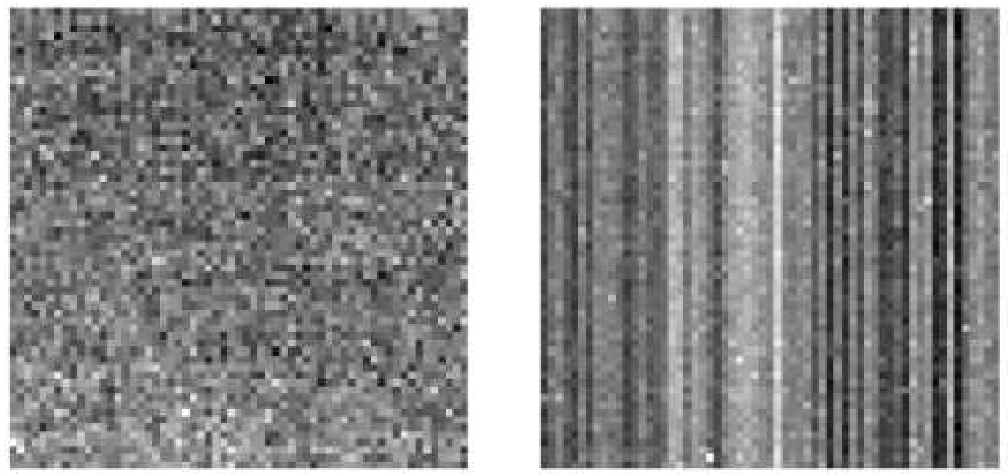
The FPN of a sensor is constant, however, it varies from sensor to sensor. In Sensors of the Charged-Coupled Device (CCD) type, the FPN varies randomly while in sensors of the Complementary Metal Oxide Semiconductor (CMOS) type, due to its perpendicular capture system, the FPN forms vertical bars, as can be seen in
Figure 1 taken from [
32].
Virtually all sensors, including the two popular examples presented earlier, produce patterns in their images that can be used for image manipulation detection. This detection is carried out by identifying areas that do not present the pattern correctly, so before detection, it is necessary to first determine the FPN produced by the camera that captured the image, a possible approach for this is to take the average of several images captured by the same camera [
30].
The work by [
33] assumes that the FPN information of the camera used for capture is previously known and then calculates the FPN of the image for validation by comparing the two and marking significantly different areas as being possibly altered.
On the other hand, methods based on classifiers use filtered features to determine if there is a correlation between parts of the image or alteration of the compression through machine learning [
34]. In deep learning [
35,
36,
37], convolutional neural networks (CNNs) are increasingly being used for image classification [
38,
39,
40].
In this field, several authors are working to reduce the complexity of the classification considering the use of big data [
41,
42,
43] and make this evaluation more efficient [
44,
45,
46] Finally, correlation-based methods compare a set of features by similarity to determine whether they contain Duplication, often using a final step to eliminate a portion of the found correlations. In this context unsupervised learning methods are also applied [
47].
All datasets found in the literature review focus on detecting Duplication and Splicing manipulations. Their most significant divergences are the images used for alteration, the size of the altered area, and the application of subsequent modifications to hide falsification on the manipulated areas. The work by [
48], which is the only one focused on detecting manipulation retouching, had to create its dataset for validation. The datasets used by analyzed works focused only on the detection of Duplication type are MICC-F220, MICC-F600, MICC-F, MICC-F2000, MICC-F8multi, IMD, CMH, CoMoFoD, and UCID.
The datasets containing Duplication and Splicing manipulations used were: CASIA v1.0, CASIA v2.0, Columbia, and Image Manipulation Database, Columbia and CASIA v1.0 datasets. Finally, the Image Manipulation Database contains a set of unaltered images and software to perform Duplication and Splicing manipulations, as well as Retouch under the areas, to be altered to hide modifications automatically, so the final adulterated images of the dataset may vary depending on usage of the software.
The problem in comparing methods for passively detecting falsified images was the limitations found in the literature. For example, some methods only detect one type of manipulation, others only work on specific types of image files, and some require or assume additional image information, such as the FPN of the camera used in the capture.
In addition to these limitations of scope, another impacting factor is the robustness of the methods; performing multiple manipulations on images tends to affect the Accuracy of different methods in different ways. This brings another problem: many datasets are available for testing with different focuses, even when trying to detect a specific type of manipulation, in addition to creating new datasets by some authors to evaluate their results.
From the comparison of the works analyzed we conclude that there is no consensus regarding ideal methods of feature extraction and image authenticity classification. Multiple approaches are possible even for identical types of manipulation, such as methods with feature extraction blocks and key points being successfully employed by different authors.
In addition, the lack of a standard dataset in all these works makes it difficult to compare the effectiveness of all methods using only the Accuracy reported by the authors, demonstrating the importance of the present work.
The problem in comparing methods for passively detecting falsified images was the limitations found in the literature. For example, some methods only detect one type of manipulation, others only work on specific types of image files, and some require or assume additional image information, such as the FPN of the camera used in the capture.
In addition to these limitations of scope, another impacting factor is the robustness of the methods. For example, multiple manipulations of images affect the Accuracy of different methods in different ways. Another problem is the number of datasets available for testing with different focuses, even when trying to detect a specific type of manipulation.
From the comparison of the works analyzed, we conclude that there needs to be more consensus in the literature regarding ideal methods of feature extraction and image authenticity classification.
In addition, the lack of a standard dataset in all these works makes it difficult to compare the effectiveness of all methods using only the Accuracy reported by the authors, demonstrating the importance of the present work.
3. Materials and Methods
3.1. Error-Level Analysis
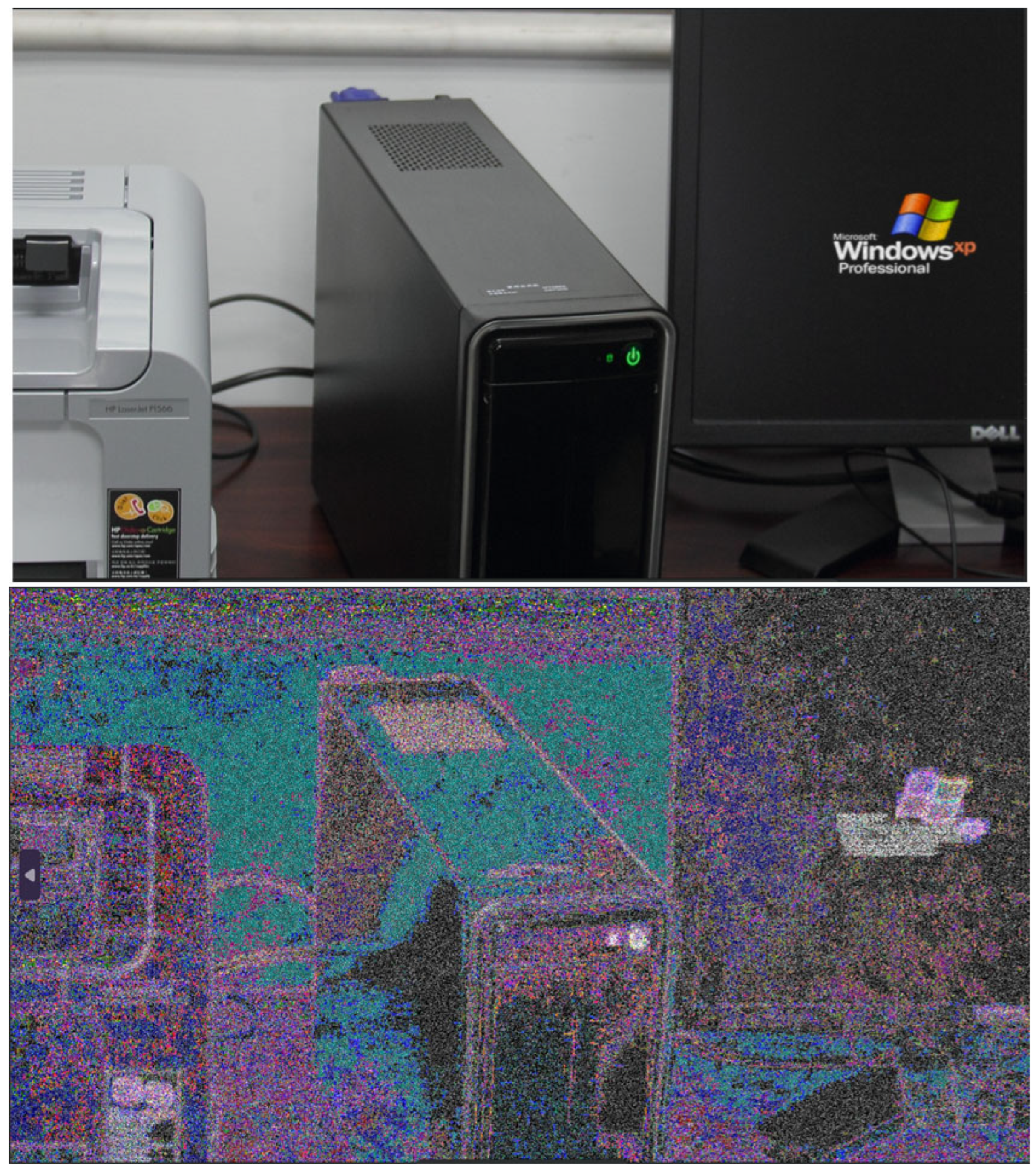
Error-Level Analysis is a passive detection method traditionally used by human forensics specialists to make differences in format artifacts of jpeg images more evident, it works by taking the difference between a jpeg image at different quality levels, making any difference in compression rate more evident on the resulting image [
48], an example of this process can be seen in the
Figure 2 and the code used to generate the images is presented in Listing 1.
|
Listing 1. Error-Level analysis implementation in pseudocode |
# Static method that performs Error Level Analysis (ELA) on an image using JPEG compression.
# Returns a normalized difference image between the original image and a JPEG-compressed version of the image.
FUNCTION method_1_ela(image, quality)
# Create another image with jpeg compression of the given quality
save_image_as_jpeg(image, temp_image, quality)
compressed_image = open_image(temp_image)
# Calculate the image difference between the original and the JPEG-compressed image
difference_image = image - compressed_image
# Normalize the difference image for contrast by assigning a value of 255 to the brightest points, while proportionally adjusting the values of all other points based on their distance from the brightest point.
normalized_difference = difference_image.normalizeContrast()
RETURN normalized_difference
END FUNCTION
|
In this example, the resulting image on the bottom is mostly black, but edited areas have more color in them, however, ELA results aren’t always so easily interpreted and traditionally need a forensics specialist to look at the results, however, this paper proposed using ELA as a feature extraction step and feeding it to a Convolutional Neural Network in order to perform the authenticity analysis of an image automatically.
3.2. Discrete Wavelet Transform
Discrete Wavelet Transform (DWT) stands for denoising [
49], which is a mathematical technique used for analyzing signals that can be applied to images [
50]. It is a way of decomposing an image into a set of frequency components, with each component representing a different level of detail or resolution [
51].
In image manipulation detection, DWT is often used for feature selection as it allows for efficient compression of image data while preserving important image features. The DWT algorithm works by dividing an image into four smaller blocks or "sub-bands" of different frequencies: The LL (low-low) sub-band, which contains the low-frequency information, and the LH (low-high), HL (high-low), and HH (high-high) sub-bands, which contain the high-frequency information [
52].
The equations to perform DWT can be found in Eq.
1 and Eq.
2 and the equation to reverse the process known as inverse DWT is presented in Eq.
3.
This work uses the technique proposed by [
53], referred to in the rest of this work as DWT method for abbreviation purposes, which makes use of DWT, Bilateral Filters, and the Laplace operator to remove less meaningful features of an image, resulting in an image only with features containing sharp pixel variation, which is a common indicator of forgery.
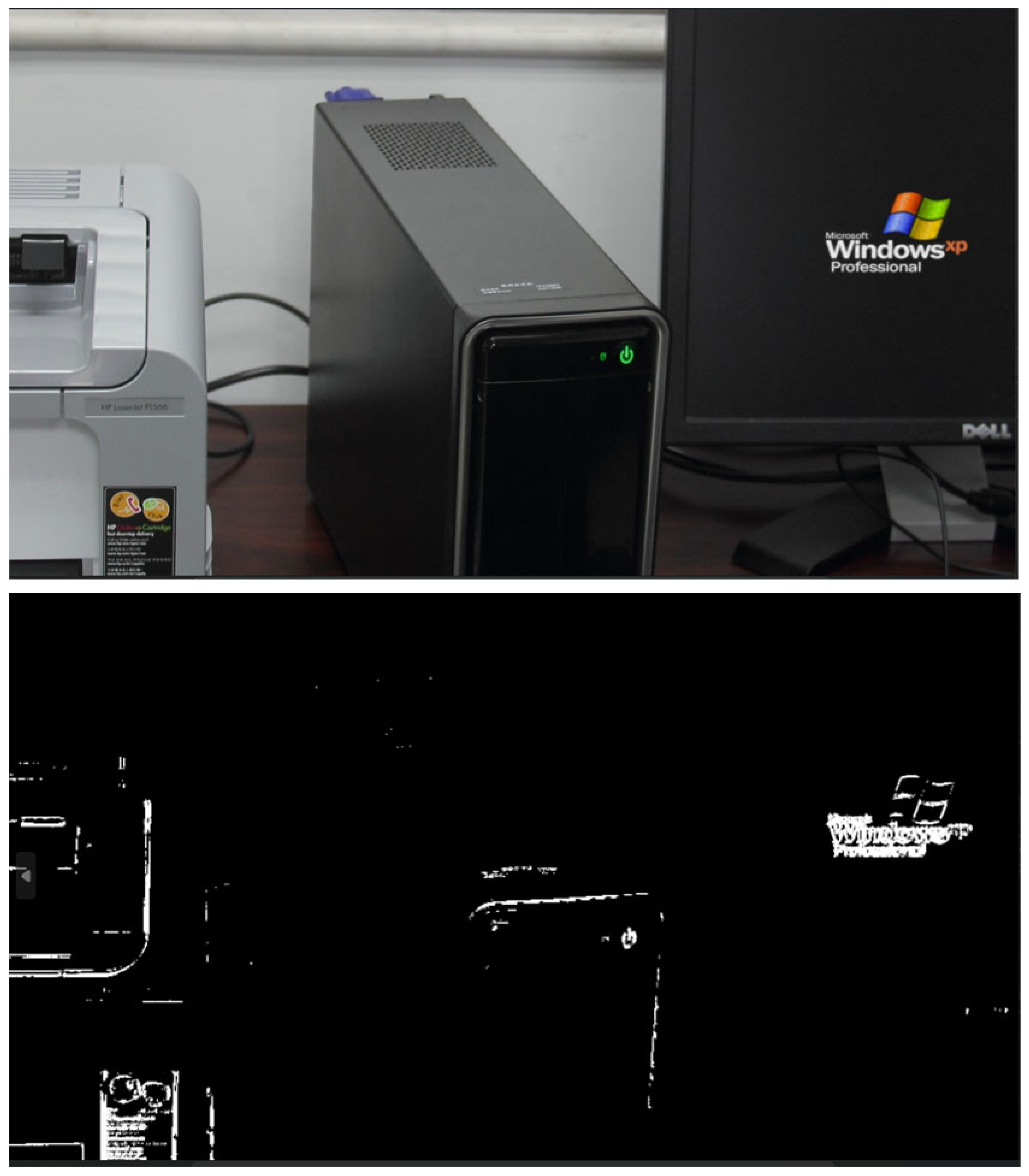
This technique works by initially the image is converted to grayscale, then DWT is applied to decompose the image information into sub-bands, then the image is reconstructed after discarding the LL band and a bilateral filter, and the Laplace operator is applied, the result is an image where sharp pixel transitions are more easily visible, however when filters are used to mask the manipulation this method fails to highlight the manipulated areas. This work uses the image resulting from this method as a feature selection step for a Convolutional Neural Network to teach it to better detect large pixel transitions.
An example of the result of this process can be seen in
Figure 3 that was taken from the RTD and the code used to generate the images is presented in Listing 2.
|
Listing 2. DWT based method implementation in pseudocode |
FUNCTION method_2_dwt(image)
# Convert image to grayscale and perform discrete wavelet transform
gray_image = convertToGrayscale(image)
coeffs = discreteWaveletTransform(gray_image)
(LL, (LH, HL, HH)) = coeffs
# Reconstruct the image using only the high-frequency components
high_freq_components = (None, (LH, HL, HH))
joinedLhHlHh = inverseDiscreteWaveletTransform(high_freq_components)
# Apply bilateral filter to smooth the image while preserving edges
blurred = bilateralFilter(joinedLhHlHh, 9, 75, 75)
# Apply Laplacian edge detection to highlight edges
kernel_size = 3
imgLapacian = laplacianEdgeDetection(blurred, kernel_size)
# Convert negative values to zero
final_image = convertScaleToAbs(imgLapacian)
RETURN final_image
END FUNCTION |
3.3. Proposed Method
The proposed approach first consists of applying the ELA method and the method proposed by [
53], both used as a feature selection step to generate two extra sets of images.
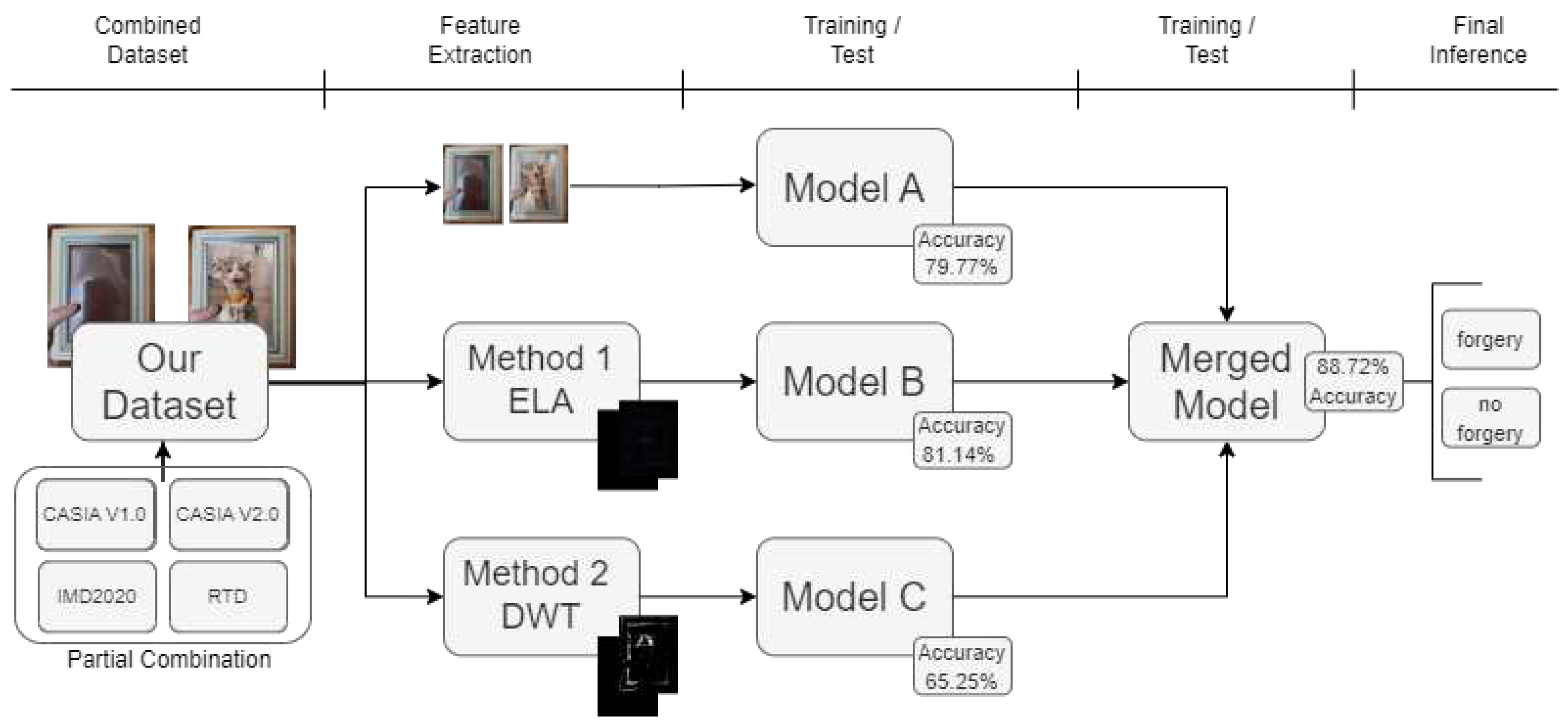
Next, the original dataset and the two new sets of images are shuffled and used for training and evaluation of three different CNNs; the three models are then frozen to preserve the acquired knowledge and merged. Finally, we added two new layers and trained them to combine the knowledge of the three models. These steps are summarized in
Figure 4, showing the overview of the system.
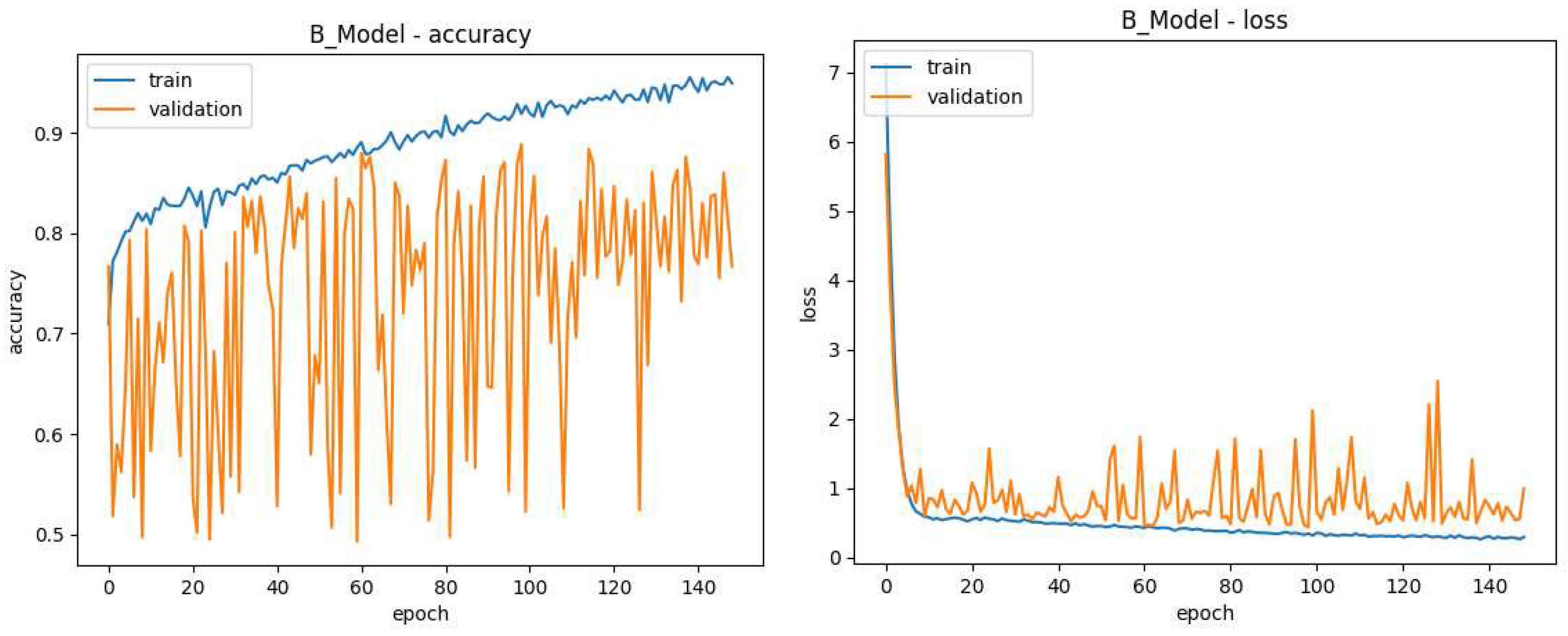
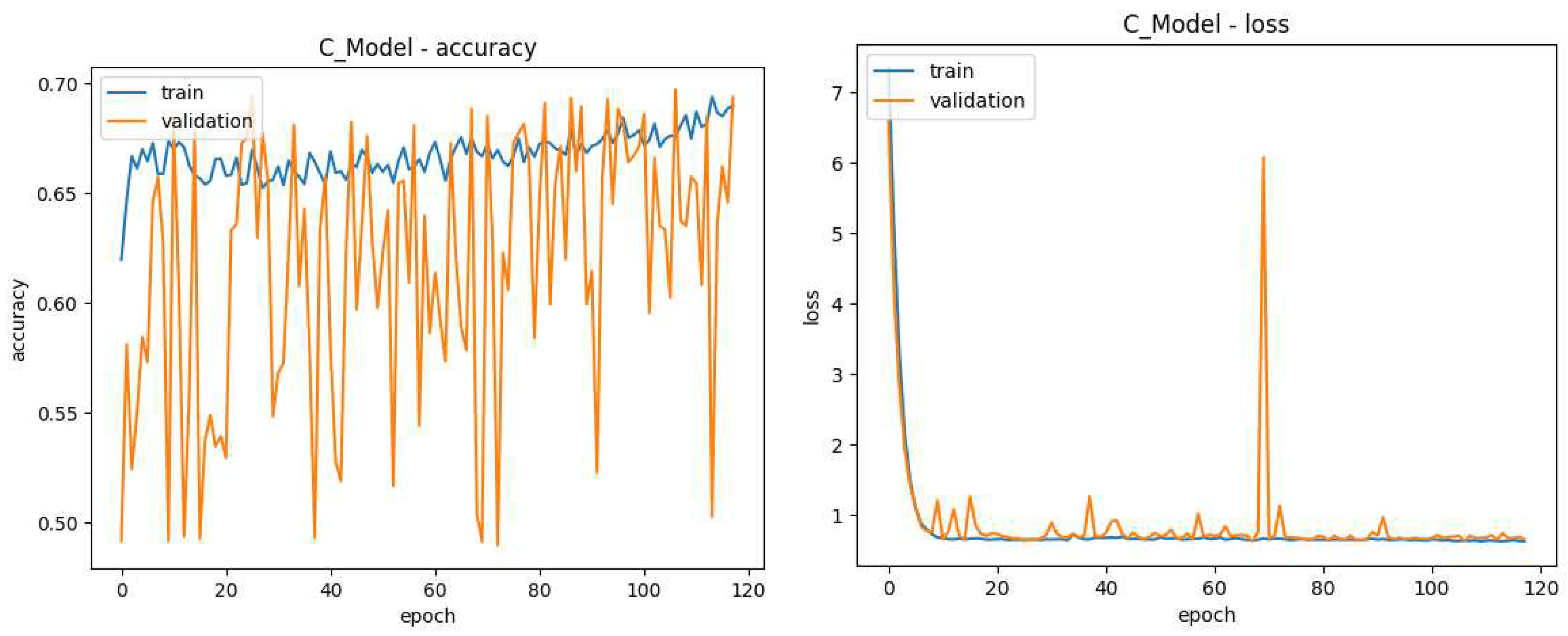
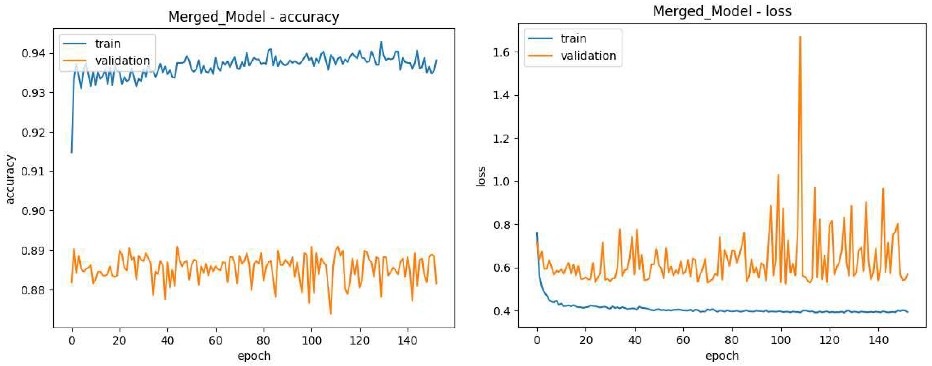
This approach aims to explore the Accuracy of each method individually in addition to their combination. For this, we individually trained three distinct models and a model composed of all three, plus additional learning layers. Model A uses only the original images without alterations as input, Model B uses only images with feature selection by ELA, and Model C uses only images with feature selection by the DWT-based method. Finally, the models are combined and four layers are added to generate the Merged model, which uses images of all three types for input.
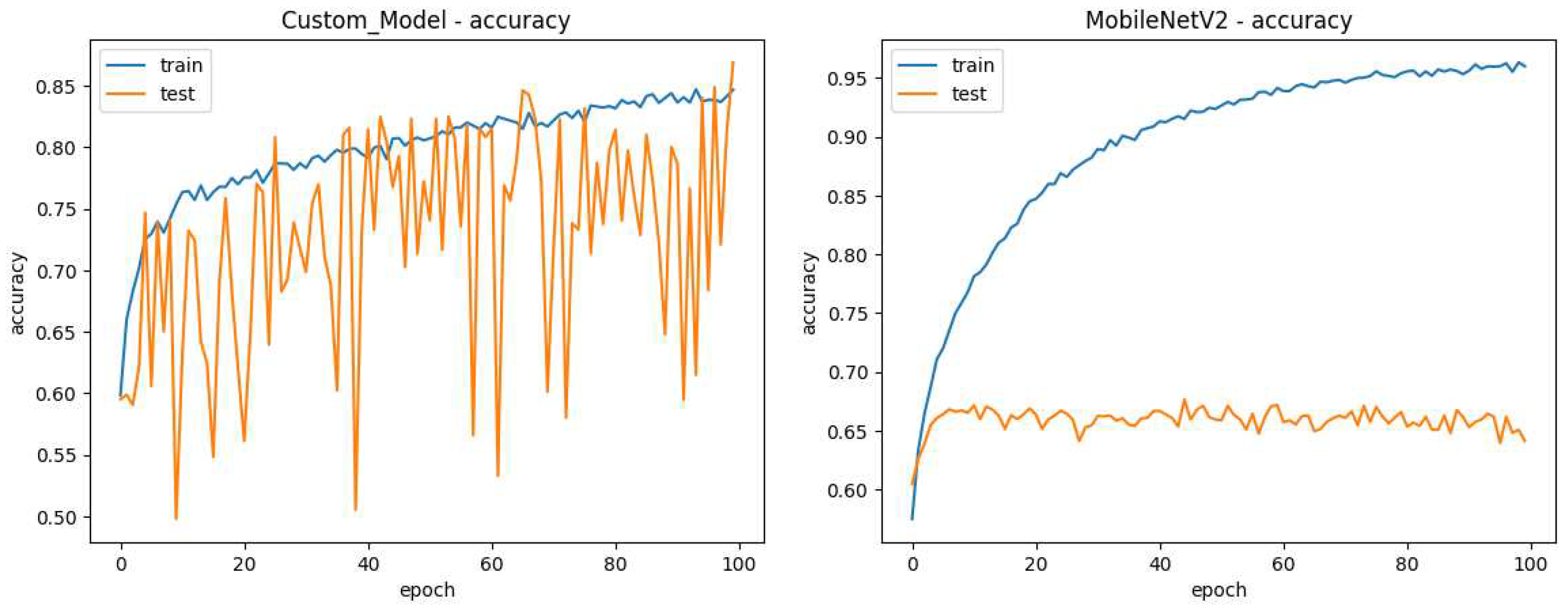
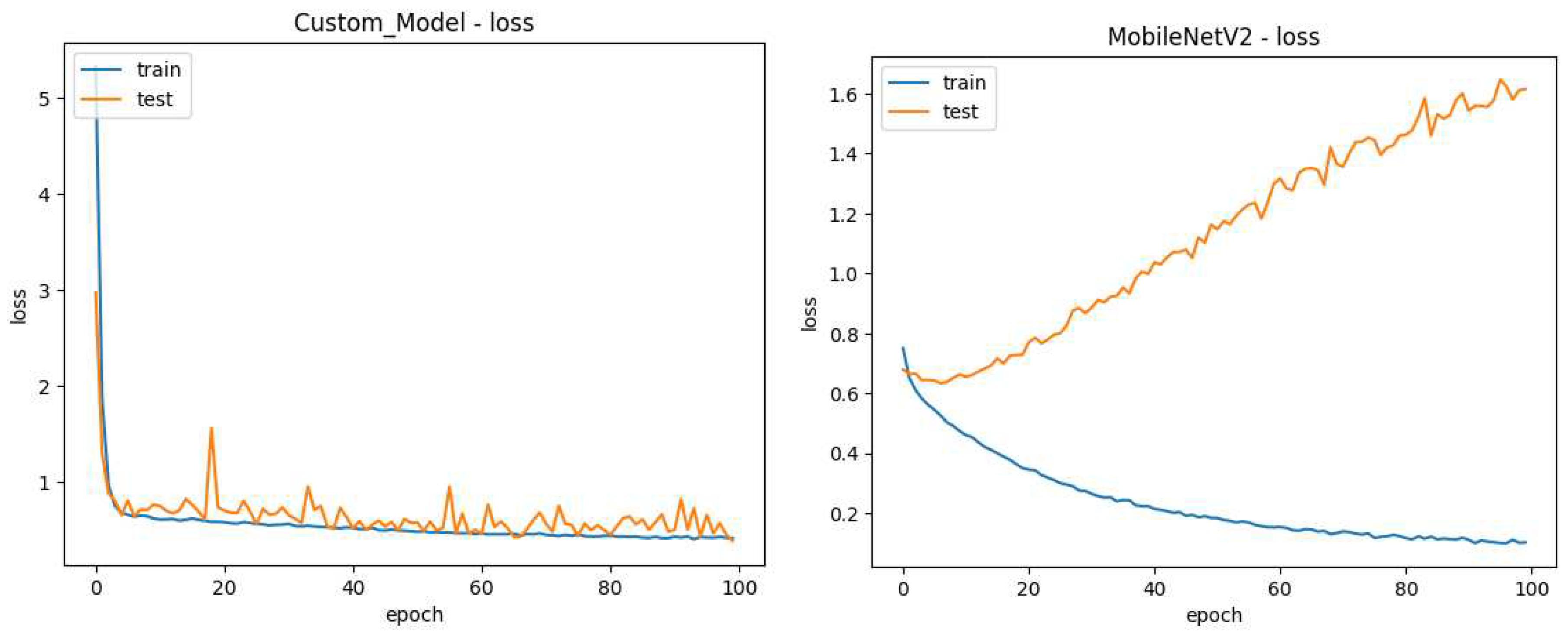
Initially, we considered the use of pre-trained models for combining the passive methods in this research. To get an initial idea of their performance concerning custom models the MobileNetV2 pre-trained model was selected for initial tests for being considered lightweight with other pre-trained models. A comparison of model performance between model "A" detailed later and MobileNetV2 plus four dense layers with l2 regularization, each followed by a batch normalization layer can be seen in the
Figure 5 and
Figure 6.
Those tests show a tendency of pre-trained models to over-fit to the training images, unfreezing some of the pre-trained layers was also attempted with similar results, the use of another pre-trained model in InceptionResNetV2 also did not yield better results than the custom model, this leads the researchers to believe pre-trained are not a good fit for image manipulation detection.
With that in mind, we decided to create three identical custom CNNs and implement regularization methods to minimize overfitting to produce results capable of generalizing to a more extensive set of images and facilitating the comparison of the three individual models.
The primary challenge in developing the neural networks for this study was addressing the issue of overfitting, where the models tend to perform well on training data but struggle to generalize to new, unseen data. To mitigate this, various experiments were conducted to assess the impact of different model architectures on accuracy.
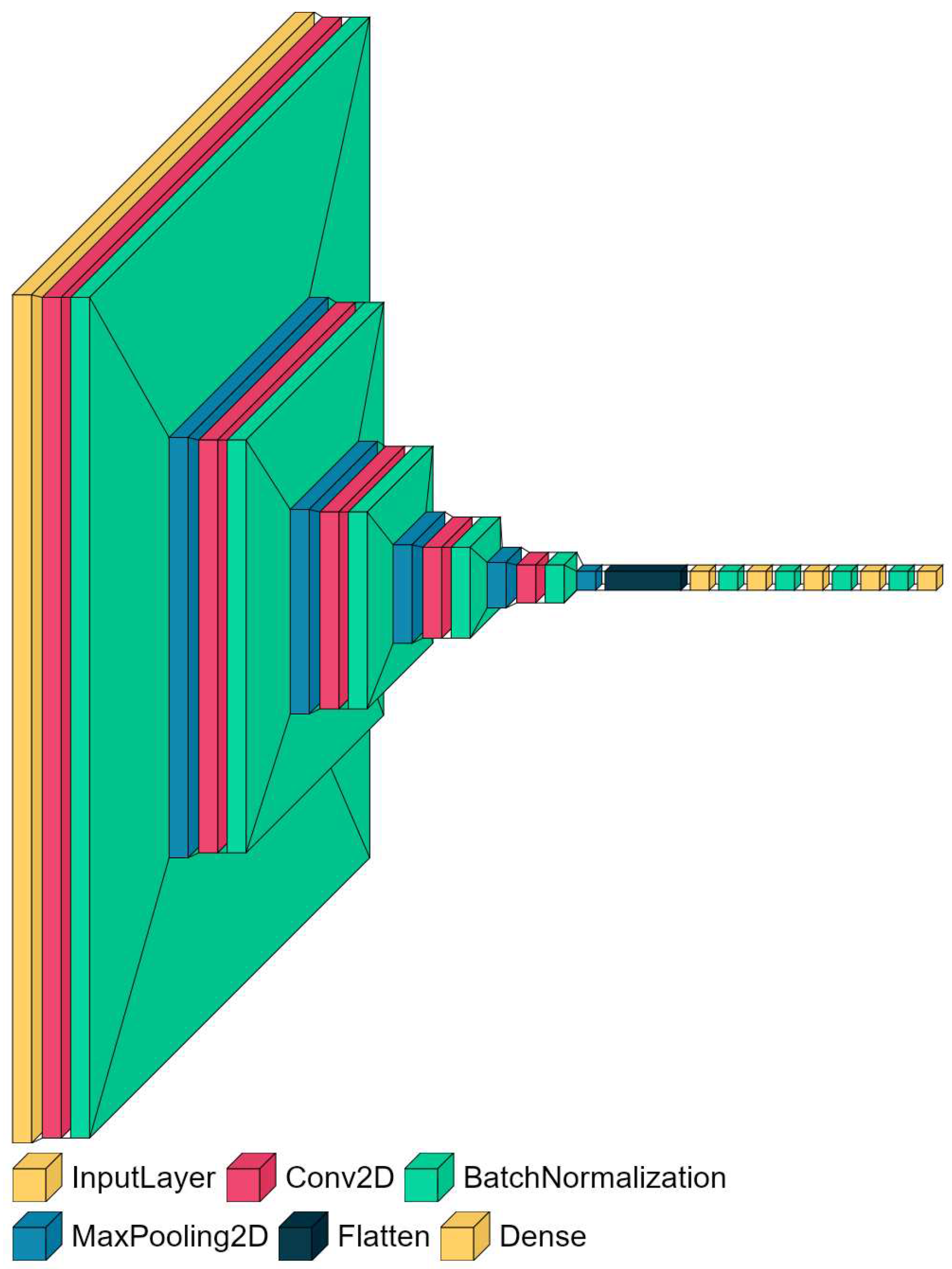
After testing multiple models with numerous layers, it was observed that increasing the number of layers did not significantly improve accuracy. Instead, it led to a higher risk of overfitting. As a result, a decision was made to design a model that consists of five convolutional layers, each followed by a batch normalization layer and a max pooling layer. The outputs from these layers were then flattened and passed through four dense layers, each accompanied by a batch normalization layer. Furthermore, L2 regularization was applied to both the convolutional and dense layers to prevent overfitting.
Figure 7 provides a visual representation of this model architecture.
The values used for the size of convolutional layers are 16,32,64,128,64 all with a 3 by 3 kernel, and the values for the dense layers are 128,128,64,32.
The final merged model that is proposed here consists of merging the individual models, initially, models A and B last non-output layer are combined through a concatenation layer, and then this combination is further merged with model C last non-output layer through another concatenated layer, then two dense layers with 64 neurons were added for learning, each followed by a batch normalization layer, all layers of the individual models were frozen to preserve the knowledge they acquired during training.
The use of Dropout layers was explored, however, Batch Normalization had a better performance given the same training time [
54]. The optimizer used was Adam, the metric during training was accuracy, and the Loss function used was Binary Cross Entropy. The activation function used was Rectified Linear Unit in all layers except in output, where we use the sigmoid Function.
3.4. Dataset Assembly
The first step to executing the experiments we carried out was assembling the final dataset, to accomplish this, we gathered authentic and manipulated images from four different datasets as explained below:
CASIA V2.0: proposed in [
55], contains 7491 authentic images and 5123 manipulated images containing Splicing and or Duplication operations with retouching operations applied on top to mask alterations;
Realistic Tampering Dataset: Proposed by [
56,
57] containing 220 authentic and 220 Splicing and or Duplication manipulations made to the original images with the objective of being realistic. Retouching operations are sometimes applied to help hide Compositing and Duplication manipulations. In addition, this dataset provides masks of tampered areas and information about capture devices used;
IMD2020: Proposed by [
58], it consists of four parts, first a dataset containing 80 authentic images manipulated to generate 1930 images tampered realistically and using all types of manipulation, with their respective manipulation masks. Then the second part consists of 35,000 authentic images captured by 2,322 different camera models, the images were collected online and reviewed manually by the authors. The third has 35,000 algorithmically generated images with retouching manipulations. Finally, the last part has 2759 authentic images acquired by the authors with 19 different camera models designed for sensor noise analysis;
CASIA V1.0: Proposed in [
55], Contains 800 authentic images, 459 Duplicate-type manipulation images, and 462 Splicing images. This dataset has no retouching operations applied.
To balance the dataset and use images manipulated realistically, we separated the images into two folders. The first contains 7491 authentic images from the CASIA V2.0 dataset. The second with manipulated images contains 7491 tampered images taken from the part from the IMD2020 dataset with Realistic Images, Realistic Tampering Dataset (RTD), CASIA V2.0, and 218 images selected from CASIA V1.0 to balance the dataset.
Table 2 shows the distribution of images used from each dataset.
Therefore, as explained in
Table 2 the final dataset used in this paper consists of 14982 images in total, half original and half Manipulated, since some of the images were not supported by model all images were converted to .jpg format.
The second step of the final program is to apply the methods described to the dataset, as both methods generate an image as output. The result is two new sets of images with specific inconsistencies enhanced, using methods from the TensorFlow library whenever applicable.
The dataset was divided into three parts: 70% for training, 20% for validation, and 10% for testing. Each image was resized to 224 by 224 pixels to match the input size required by MobileNetV2, a pre-trained neural network that was initially considered but ultimately not used in favor of a custom model due to improved performance.
The experiment consisted of first creating two additional sets of images using the two selected passive methods. Subsequently, three convolutional neural networks were trained: Model A using the original dataset, and Models B and C utilizing the outputs of the selected passive methods. These models were then combined by concatenating them at the penultimate layer. Additionally, an extra dense layer followed by a batch regularization layer was introduced so the model could learn how to combine the results, this combination is the final merged model.
To enhance accuracy and mitigate overfitting, three techniques were employed. First, a model checkpoint callback was implemented, which saved the model weights corresponding to the minimum validation loss achieved during training. Second, an early stopping condition was defined, terminating training after 50 epochs without any improvement in validation loss.
The third technique used to reduce overfitting was the use of dataset augmentation techniques applied at the end of every epoch to the training images, which randomly flipped the image in the four-axis and changed the brightness, contrast, saturation, and hue of the images randomly.
The experiments were conducted on a system with the following specifications: Windows 11 operating system, Intel(R) Core(TM) i5-8300H CPU 2.30GHz, 16GB RAM, GeForce GTX 1050 graphics card, Python version 3.10, CUDA version 11.2, cuDNN version 8.1.1, and TensorFlow version 2.10.0. The training was performed with a batch size of 32 over a total of 500 epochs, as the dataset exhibited significant variation in manipulations, leading to fluctuation in the loss of validation images.
4. Results and Discussion
After training, the final Accuracy obtained by the merged model was 89,59% in the set of test images, higher than the model trained just with original images, which obtained 78.64%.
The final results obtained after the stop conditions were triggered are on the
Table 3 below.
5. Conclusion and Future Work
This work offered a review of how forensic methods for detecting manipulated images work and applied two detection methods and a mixture of both using CNNs to a dataset containing a diverse set of manipulations.
After training, the proposed merged method obtained an accuracy of 89.59% in the validation images, significantly higher than the model trained with original images, which obtained 78.64%, and the model that enhances compression differences in images using ELA which obtained 68.02% and the worst performing model individually that uses the method proposed by [
53] with 50.70%.
The combination of models trained differently but on the same set of images in this work demonstrates the possibility of using techniques from the detection of falsified images to guide Neural Network models to learn different detection techniques. We observed this in the final model that obtained an Accuracy higher than all the models used for its creation.
With the proposed approach, the research could serve as a basis for the elaboration of future works about the detection of manipulated images that contain different approaches, nomenclatures, and possible methods that were generalized to structure the knowledge available in this field.
The proposed method opens several possibilities for future work. For example, it is possible to cite them as the combination and comparison of more trained models with different selection or feature extraction methods, testing other model architectures like you only look once (YOLO), modifications to the model to localize the manipulated area and tests of the proposed method on other sets of images. In future work, we also intend to optimize the algorithms used, compare the results, and evaluate them in other scenarios. When it comes to the safety of the data used, it will also be necessary to carry out studies and define future criteria and parameters for this issue. Energy consumption, quantity, and size of data used is something interesting to be investigated in future work, with this and other various hypotheses that may arise, several improvements and future contributions may result.
Author Contributions
Writing—original draft, A.C.R.K.; writing—review and editing, software, methodology, validation, L.O.S. J.C.A; writing—review and editing, V.C.M.; supervision, L.d.S.C.; V.R.Q.L. All authors have read and agreed to the published version of the manuscript.
Funding
The authors Mariani and Coelho thank the National Council of Scientific and Technologic Development of Brazil — CNPq (Grants number: 314389/2023-7-PQ, 313169/2023-3-PQ, 407453/2023-7-Universal, and 442176/2023-6-Peci), and Fundação Araucária PRONEX Grant 042/2018 for its financial support of this work. The author Seman thanks the National Council of Scientific and Technologic Development of Brazil — CNPq (Grant number: 308361/2022-9). This research was funded by national funds through the Fundação para a Ciência e a Tecnologia, I.P. (Portuguese Foundation for Science and Technology) by the project UIDB/05064/2020 (VALORIZA-Research Centre for Endogenous Resource Valorization) and it was partially supported by Fundação para a Ciência e a Tecnologia under Project UIDB/04111/2020, and ILIND–Instituto Lusófono de Investigação e Desenvolvimento, under projects COFAC/ILIND/COPELABS/1/2020 and COFAC/ILIND/COPELABS/3/2020.
Informed Consent Statement
Not applicable.
Data Availability Statement
It can be provided upon request.
Conflicts of Interest
The authors declare no conflict of interest.
Abbreviations
The following abbreviations are used in this manuscript:
| CID |
Content identifier |
| CNN |
Convolutional neural network |
| COV |
computer vision |
| DEL |
Deep learning |
| DIF |
Digital image forensics |
| DWT |
Discrete Wavelet Transform |
| IMP |
Image processing |
| FP |
False positive |
| FN |
False negative |
| HCI |
Human-computer interaction |
| MLP |
Multilayer perceptron |
| R-CNN |
Region-based convolutional neural networks |
| RI |
Region of interest |
| RPN |
Region proposal network |
| TC |
Totally connected |
| TF |
True negative |
| TP |
True positive |
References
- Lazer, D.M.J.; Baum, M.A.; Benkler, Y.; Berinsky, A.J.; Greenhill, K.M.; Menczer, F.; Metzger, M.J.; Nyhan, B.; Pennycook, G.; Rothschild, D.; Schudson, M.; Sloman, S.A.; Sunstein, C.R.; Thorson, E.A.; Watts, D.J.; Zittrain, J.L. The science of fake news. Science 2018, 359, 1094–1096. [Google Scholar] [CrossRef]
- The Anatomy of a Scientific Rumor - Scientific Reports — nature.com. https://www.nature.com/articles/srep02980. [Accessed 04-Feb-2023].
- Nash, R.A.; Wade, K.A.; Lindsay, D.S. Digitally manipulating memory: Effects of doctored videos and imagination in distorting beliefs and memories. Memory & Cognition 2009, 37, 414–424. [Google Scholar] [CrossRef]
- López-Cantos, F. The Impact on Public Trust of Image Manipulation in Science. Informing Science: The International Journal of an Emerging Transdiscipline 2019, 22, 045–053. [Google Scholar] [CrossRef] [PubMed]
- Liu, B.; Pun, C.M. Exposing splicing forgery in realistic scenes using deep fusion network. Information Sciences 2020, 526, 133–150. [Google Scholar] [CrossRef]
- Rocha, A.; Scheirer, W.; Boult, T.; Goldenstein, S. Vision of the unseen. ACM Computing Surveys 2011, 43, 1–42. [Google Scholar] [CrossRef]
- Sharma, V.; Jha, S. Image Forgery and it’s Detection Technique: A Review. 2016.
- Qazi, T.; Hayat, K.; Khan, S.U.; Madani, S.A.; Khan, I.A.; Kołodziej, J.; Li, H.; Lin, W.; Yow, K.C.; Xu, C.Z. Survey on blind image forgery detection. IET Image Processing 2013, 7, 660–670. [Google Scholar] [CrossRef]
- Lubna, J.I.; Chowdhury, S.M.A.K. Detecting Fake Image: A Review for Stopping Image Manipulation. Advances in Computational Intelligence, Security and Internet of Things; Saha, A.; Kar, N.; Deb, S., Eds., 2020, pp. 146–159. [CrossRef]
- Sharma, S.; Ghanekar, U. A hybrid technique to discriminate Natural Images, Computer Generated Graphics Images, Spliced, Copy Move tampered images and Authentic images by using features and ELM classifier. Optik 2018, 172, 470–483. [Google Scholar] [CrossRef]
- Agarwal, R.; Khudaniya, D.; Gupta, A.; Grover, K. Image Forgery Detection and Deep Learning Techniques: A Review. 2020 4th International Conference on Intelligent Computing and Control Systems (ICICCS), 2020, pp. 1096–1100. [CrossRef]
- Dua, S.; Singh, J.; Parthasarathy, H. Detection and localization of forgery using statistics of DCT and Fourier components. Signal Processing: Image Communication 2020, 82, 115778. [Google Scholar] [CrossRef]
- Vaishnavi, D.; Subashini, T. Application of local invariant symmetry features to detect and localize image copy move forgeries. Journal of Information Security and Applications 2019, 44, 23–31. [Google Scholar] [CrossRef]
- Lyu, Q.; Luo, J.; Liu, K.; Yin, X.; Liu, J.; Lu, W. Copy Move Forgery Detection based on double matching. Journal of Visual Communication and Image Representation 2021, 76, 103057. [Google Scholar] [CrossRef]
- Mahmood, T.; Mehmood, Z.; Shah, M.; Saba, T. A robust technique for copy-move forgery detection and localization in digital images via stationary wavelet and discrete cosine transform. Journal of Visual Communication and Image Representation 2018, 53, 202–214. [Google Scholar] [CrossRef]
- Kasban, H.; Nassar, S. An efficient approach for forgery detection in digital images using Hilbert–Huang transform. Applied Soft Computing 2020, 97, 106728. [Google Scholar] [CrossRef]
- Hashmi, M.F.; Hambarde, A.R.; Keskar, A.G. Copy move forgery detection using DWT and SIFT features. 2013 13th International Conference on Intellient Systems Design and Applications, 2013, pp. 188–193. [CrossRef]
- Malviya, A.V.; Ladhake, S.A. Region duplication detection using color histogram and moments in digital image. 2016 International Conference on Inventive Computation Technologies, 2016, Vol. 1, pp. 1–4. [CrossRef]
- Sanap, V.K.; Mane, V.M. Region duplication forgery detection in digital images using 2D-DWT and SVD. 2015 International Conference on Applied and Theoretical Computing and Communication Technology (iCATccT), 2015, pp. 599–604. [CrossRef]
- Khan, S.; Kulkarni, A. Robust method for detection of copy-move forgery in digital images. 2010 International Conference on Signal and Image Processing 2010, pp. 69–73. [CrossRef]
- Fahmy, M.F.; Fahmy, O.M. A natural preserving transform based forgery detection scheme. 2015 IEEE International Symposium on Signal Processing and Information Technology (ISSPIT), 2015, pp. 215–220. [CrossRef]
- Isaac, M.M.; Wilscy, M. Copy-Move forgery detection based on Harris Corner points and BRISK. Proceedings of the Third International Symposium on Women in Computing and Informatics, 2015. [CrossRef]
- Liu, Q.; Li, X.; Cooper, P.A.; Hu, X. Shift recompression-based feature mining for detecting content-aware scaled forgery in JPEG images. Proceedings of the Twelfth International Workshop on Multimedia Data Mining, 2012. [CrossRef]
- Soni, B.; Das, P.K.; Thounaojam, D.M. Blur Invariant Block based Copy-Move Forgery Detection Technique using FWHT Features. Proceedings of the International Conference on Watermarking and Image Processing, 2017. [CrossRef]
- Liu, Q.; Sung, A.H. A new approach for JPEG resize and image splicing detection. Proceedings of the First ACM workshop on Multimedia in forensics, 2009. [CrossRef]
- Li, C.; Ma, Q.; Xiao, L.; Ying, S. An Image Copy Move Forgery Detection Method Using QDCT. Proceedings of the International Conference on Internet Multimedia Computing and Service, 2016. [CrossRef]
- Liu, Y.; Guan, Q.; Zhao, X.; Cao, Y. Image Forgery Localization Based on Multi-Scale Convolutional Neural Networks 2017. [CrossRef]
- Ravi, K.; Devraj, N.; Shylaja, S.S. A new approach to detect paste forgeries in an image. 2017 Fourth International Conference on Image Information Processing (ICIIP), 2017, pp. 1–6. [CrossRef]
- Rao, Y.; Ni, J.; Xie, H. Multi-semantic CRF-based attention model for image forgery detection and localization. Signal Process. 2021, 183, 108051. [Google Scholar] [CrossRef]
- Lukáš, J.; Fridrich, J.; Goljan, M. Detecting digital image forgeries using sensor pattern noise. SPIE Proceedings; III, E.J.D.; Wong, P.W., Eds. SPIE, 2006. [CrossRef]
- Lin, X.; Li, C.T. PRNU-Based Content Forgery Localization Augmented With Image Segmentation. IEEE Access 2020, 8, 222645–222659. [Google Scholar] [CrossRef]
- Mohammadnejad, S.; Roshani, S.; Sarvi, M. Fixed pattern noise reduction method in CCD sensors for LEO satellite applications. Proceedings of the 11th International Conference on Telecommunications 2011.
- Fahmy, M.F.; Fahmy, O.M. A natural preserving transform based forgery detection scheme. 2015 IEEE International Symposium on Signal Processing and Information Technology (ISSPIT), 2015, pp. 215–220. [CrossRef]
- Stefenon, S.F.; Corso, M.P.; Nied, A.; Perez, F.L.; Yow, K.C.; Gonzalez, G.V.; Leithardt, V.R.Q. Classification of insulators using neural network based on computer vision. IET Generation, Transmission & Distribution 2021, 16, 1096–1107. [CrossRef]
- Corso, M.P.; Stefenon, S.F.; Singh, G.; Matsuo, M.V.; Perez, F.L.; Leithardt, V.R.Q. Evaluation of visible contamination on power grid insulators using convolutional neural networks. Electrical Engineering 2023, 105, 3881–3894. [Google Scholar] [CrossRef]
- Dos Santos, G.H.; Seman, L.O.; Bezerra, E.A.; Leithardt, V.R.Q.; Mendes, A.S.; Stefenon, S.F. Static attitude determination using convolutional neural networks. Sensors 2021, 21, 6419. [Google Scholar] [CrossRef]
- Souza, B.J.; Stefenon, S.F.; Singh, G.; Freire, R.Z. Hybrid-YOLO for classification of insulators defects in transmission lines based on UAV. International Journal of Electrical Power & Energy Systems 2023, 148, 108982. [Google Scholar] [CrossRef]
- Stefenon, S.F.; Yow, K.C.; Nied, A.; Meyer, L.H. Classification of distribution power grid structures using inception v3 deep neural network. Electrical Engineering 2022, 104, 4557–4569. [Google Scholar] [CrossRef]
- Lu, J.; Tan, L.; Jiang, H. Review on convolutional neural network (CNN) applied to plant leaf disease classification. Agriculture 2021, 11, 707. [Google Scholar] [CrossRef]
- Yu, C.; Han, R.; Song, M.; Liu, C.; Chang, C.I. A simplified 2D-3D CNN architecture for hyperspectral image classification based on spatial-spectral fusion. IEEE Journal of Selected Topics in Applied Earth Observations and Remote Sensing 2020, 13, 2485–2501. [Google Scholar] [CrossRef]
- Yamasaki, M.; Freire, R.Z.; Seman, L.O.; Stefenon, S.F.; Mariani, V.C.; dos Santos Coelho, L. Optimized hybrid ensemble learning approaches applied to very short-term load forecasting. International Journal of Electrical Power & Energy Systems 2024, 155, 109579. [Google Scholar] [CrossRef]
- Starke, L.; Hoppe, A.F.; Sartori, A.; Stefenon, S.F.; Santana, J.F.D.P.; Leithardt, V.R.Q. Interference recommendation for the pump sizing process in progressive cavity pumps using graph neural networks. Scientific Reports 2023, 13, 16884. [Google Scholar] [CrossRef] [PubMed]
- Surek, G.A.S.; Seman, L.O.; Stefenon, S.F.; Mariani, V.C.; Coelho, L.S. Video-based human activity recognition using deep learning approaches. Sensors 2023, 23, 6384. [Google Scholar] [CrossRef] [PubMed]
- Glasenapp, L.A.; Hoppe, A.F.; Wisintainer, M.A.; Sartori, A.; Stefenon, S.F. OCR Applied for Identification of Vehicles with Irregular Documentation Using IoT. Electronics 2023, 12, 1083. [Google Scholar] [CrossRef]
- Vieira, J.C.; Sartori, A.; Stefenon, S.F.; Perez, F.L.; de Jesus, G.S.; Leithardt, V.R.Q. Low-Cost CNN for Automatic Violence Recognition on Embedded System. IEEE Access 2022, 10, 25190–25202. [Google Scholar] [CrossRef]
- Corso, M.P.; Perez, F.L.; Stefenon, S.F.; Yow, K.C.; Ovejero, R.G.; Leithardt, V.R.Q. Classification of Contaminated Insulators Using k-Nearest Neighbors Based on Computer Vision. Computers 2021, 10, 112. [Google Scholar] [CrossRef]
- Wilbert, H.J.; Hoppe, A.F.; Sartori, A.; Stefenon, S.F.; Silva, L.A. Recency, Frequency, Monetary Value, Clustering, and Internal and External Indices for Customer Segmentation from Retail Data. Algorithms 2023, 16, 396. [Google Scholar] [CrossRef]
- Gunawan, T.S.; Hanafiah, S.A.M.; Kartiwi, M.; Ismail, N.; Za’bah, N.F.; Nordin, A.N. Development of Photo Forensics Algorithm by Detecting Photoshop Manipulation using Error Level Analysis. Indonesian Journal of Electrical Engineering and Computer Science 2017, 7, 131. [Google Scholar] [CrossRef]
- Stefenon, S.F.; Seman, L.O.; Aquino, L.S.; dos Santos Coelho, L. Wavelet-Seq2Seq-LSTM with attention for time series forecasting of level of dams in hydroelectric power plants. Energy 2023, 274, 127350. [Google Scholar] [CrossRef]
- Sopelsa Neto, N.F.; Stefenon, S.F.; Meyer, L.H.; Ovejero, R.G.; Leithardt, V.R.Q. Fault Prediction Based on Leakage Current in Contaminated Insulators Using Enhanced Time Series Forecasting Models. Sensors 2022, 22, 6121. [Google Scholar] [CrossRef] [PubMed]
- Branco, N.W.; Cavalca, M.S.M.; Stefenon, S.F.; Leithardt, V.R.Q. Wavelet LSTM for fault forecasting in electrical power grids. Sensors 2022, 22, 8323. [Google Scholar] [CrossRef] [PubMed]
- Klaar, A.C.R.; Stefenon, S.F.; Seman, L.O.; Mariani, V.C.; Coelho, L.d.S. Optimized EWT-Seq2Seq-LSTM with Attention Mechanism to Insulators Fault Prediction. Sensors 2023, 23, 3202. [Google Scholar] [CrossRef]
- Ravi, K.; Devraj, N.; Shylaja, S.S. A new approach to detect paste forgeries in an image. 2017 Fourth International Conference on Image Information Processing (ICIIP), 2017, pp. 1–6. [CrossRef]
- Singh, G.; Stefenon, S.F.; Yow, K.C. Interpretable visual transmission lines inspections using pseudo-prototypical part network. Machine Vision and Applications 2023, 34, 41. [Google Scholar] [CrossRef]
- Dong, J.; Wang, W.; Tan, T. CASIA Image Tampering Detection Evaluation Database. 2013 IEEE China Summit and International Conference on Signal and Information Processing, 2013, pp. 422–426. [CrossRef]
- Korus, P.; Huang, J. Multi-scale Analysis Strategies in PRNU-based Tampering Localization. IEEE Trans. on Information Forensics & Security 2017. [CrossRef]
- Korus, P.; Huang, J. Evaluation of Random Field Models in Multi-modal Unsupervised Tampering Localization. Proc. of IEEE Int. Workshop on Inf. Forensics and Security, 2016. [CrossRef]
- Novozámský, A.; Mahdian, B.; Saic, S. IMD2020: A Large-Scale Annotated Dataset Tailored for Detecting Manipulated Images. IEEE Winter Applications of Computer Vision Workshops, 2020, pp. 71–80. [CrossRef]
Figure 1.
Comparison of FPN present in CCD and CMOS sensors (left) FPN of a CCD sensor (right) FPN pf a CMOS sensor
Figure 1.
Comparison of FPN present in CCD and CMOS sensors (left) FPN of a CCD sensor (right) FPN pf a CMOS sensor
Figure 2.
Example of the results obtained after performing Error-Level Analysis (ELA) (top) Image with the windows logo and power button manipulated taken from RTD (bottom) Resulting image after ELA has been applied is usually mostly black, except for the two manipulated areas that have differences in compression, to make results easier to see in this paper the ELA image presented here had its brightness further enhanced by a factor of 8
Figure 3.
Example of the results obtained after performing the DWT method (top) Image with the windows logo and power button manipulated (bottom) Results of the DWT based method where sharp pixel variations are enhanced
Figure 3.
Example of the results obtained after performing the DWT method (top) Image with the windows logo and power button manipulated (bottom) Results of the DWT based method where sharp pixel variations are enhanced
Figure 4.
Illustration of the proposed approach
Figure 4.
Illustration of the proposed approach
Figure 5.
Comparing the accuracy of a custom model to MobileNetV2. (left) Custom model accuracy during training (right) Pre trained MobileNetV2 accuracy during training
Figure 5.
Comparing the accuracy of a custom model to MobileNetV2. (left) Custom model accuracy during training (right) Pre trained MobileNetV2 accuracy during training
Figure 6.
Comparing loss of a custom model to MobileNetV2. (left) Custom model loss during training (right) Pre trained MobileNetV2 loss during training
Figure 6.
Comparing loss of a custom model to MobileNetV2. (left) Custom model loss during training (right) Pre trained MobileNetV2 loss during training
Figure 7.
Illustration of the architecture used in the three individual models
Figure 7.
Illustration of the architecture used in the three individual models
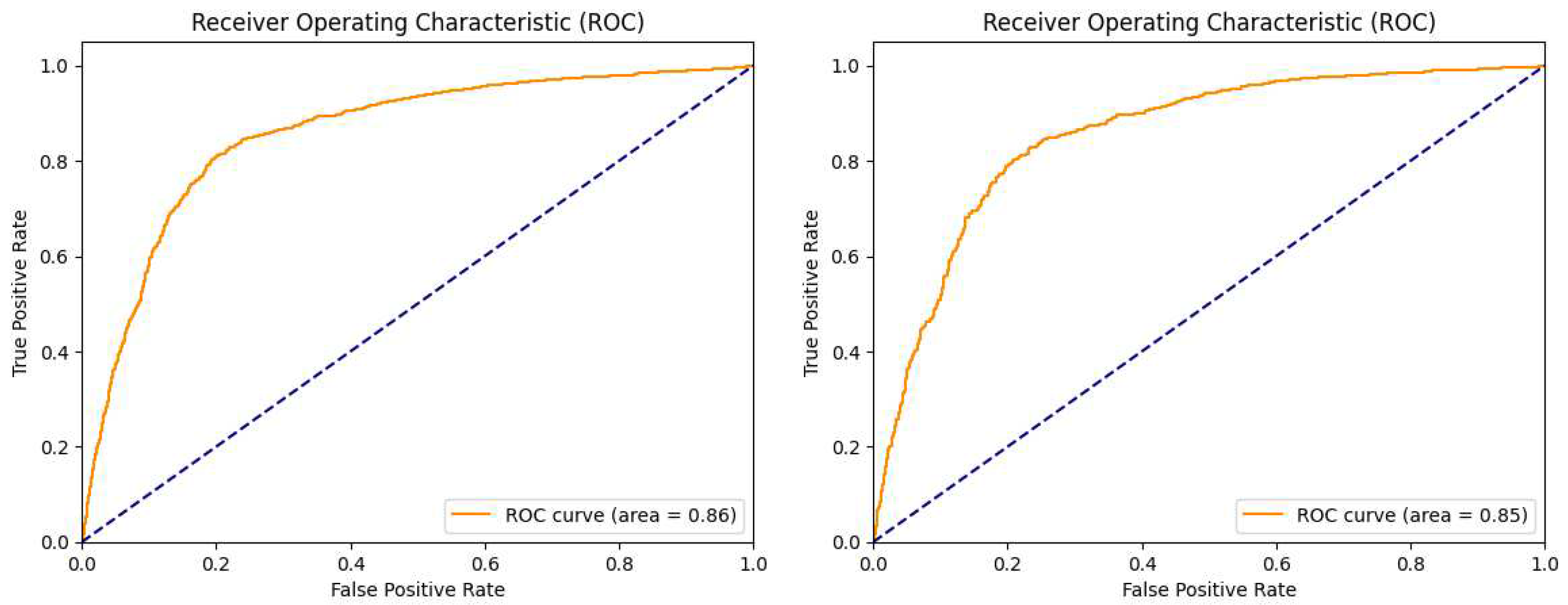
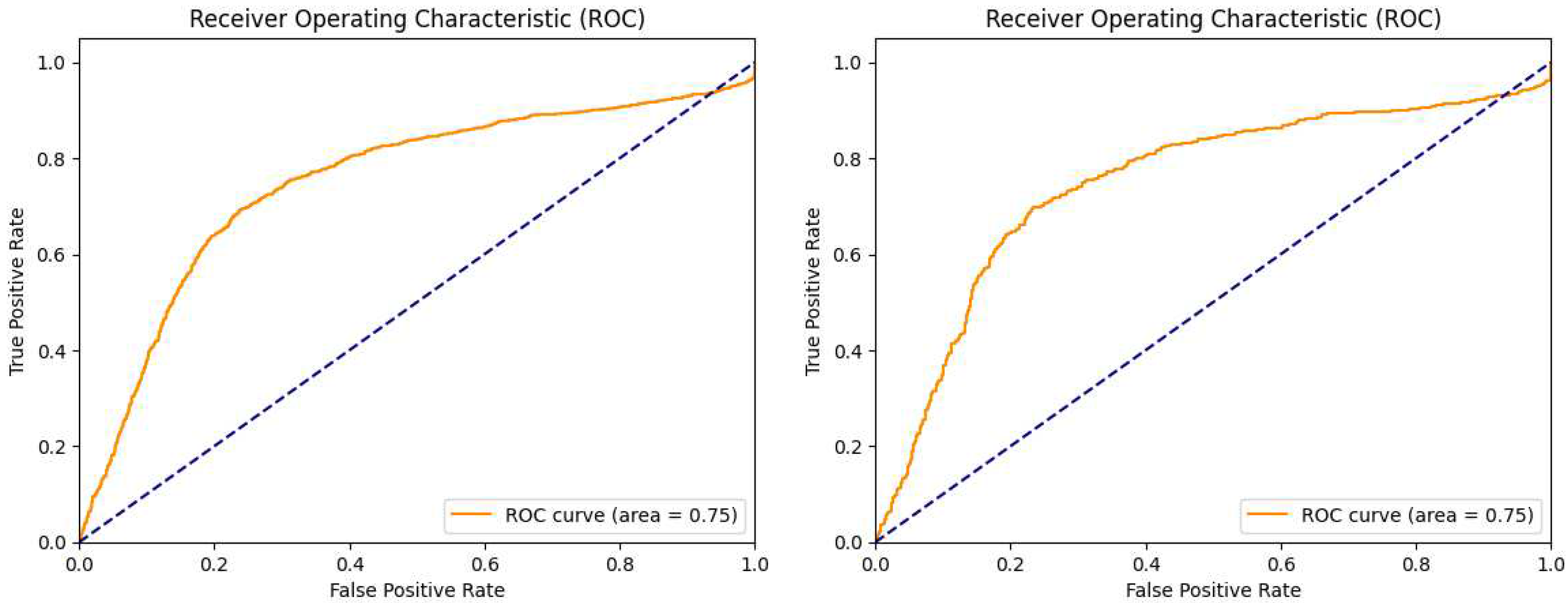
Figure 8.
Model A area under curve (ROC) for the training and test datasets. (left) Results obtained on the validation dataset. (right) Results obtained on the test dataset.
Figure 8.
Model A area under curve (ROC) for the training and test datasets. (left) Results obtained on the validation dataset. (right) Results obtained on the test dataset.
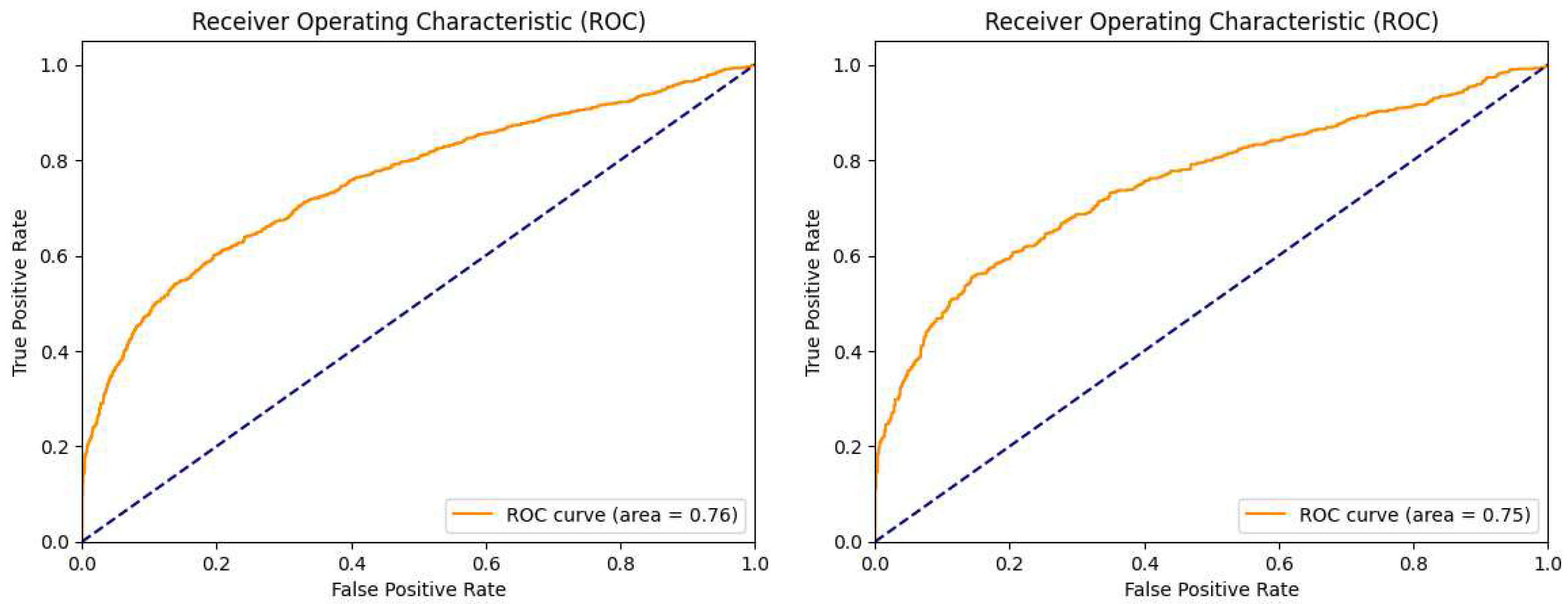
Figure 9.
Model B area under curve (ROC) for the training and test datasets. (left) Results obtained on the validation dataset. (right) Results obtained on the test dataset.
Figure 9.
Model B area under curve (ROC) for the training and test datasets. (left) Results obtained on the validation dataset. (right) Results obtained on the test dataset.
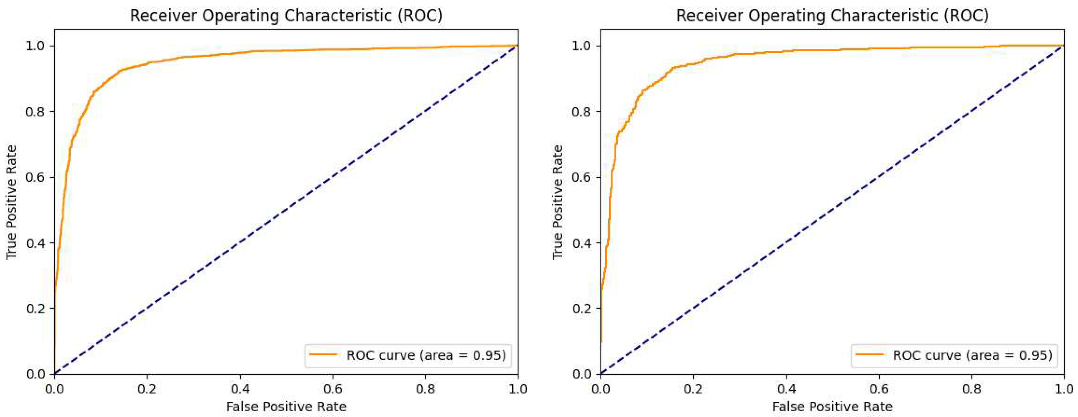
Figure 10.
Model C area under curve (ROC) for the training and test datasets. (left) Results obtained on the validation dataset. (right) Results obtained on the test dataset.
Figure 10.
Model C area under curve (ROC) for the training and test datasets. (left) Results obtained on the validation dataset. (right) Results obtained on the test dataset.
Figure 11.
Proposed Model area under curve (ROC) for the training and test datasets. (left) Results obtained on the validation dataset. (right) Results obtained on the test dataset.
Figure 11.
Proposed Model area under curve (ROC) for the training and test datasets. (left) Results obtained on the validation dataset. (right) Results obtained on the test dataset.
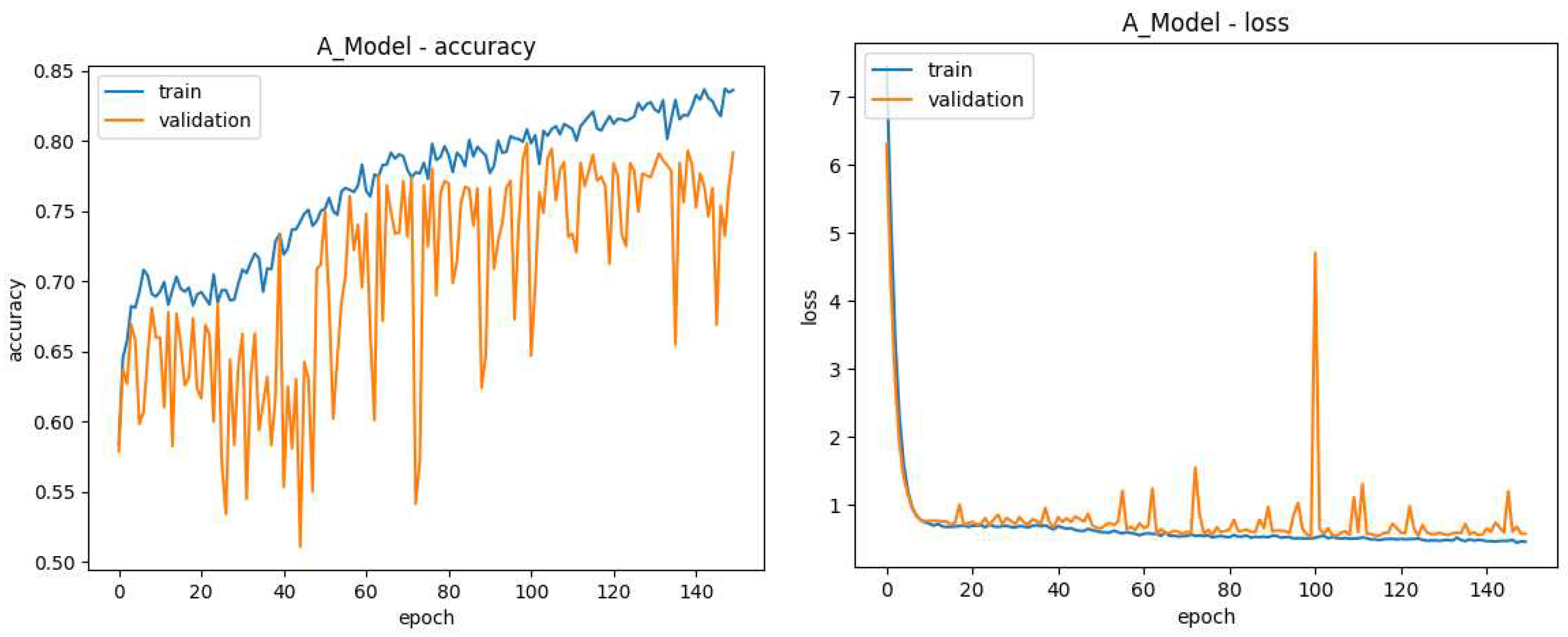
Figure 12.
Model A Training Data, the lines in blue refer to results on the 80% of images used for training while those in orange refer to the 20% of images dedicated to validation. The X-axis shows the current training generation. (left) Y-axis shows Accuracy during model A training (right) Y-axis shows loss during model A training.
Figure 13.
Model B Training Data, the lines in blue refer to results on the 80% of images used for training while those in orange refer to the 20% of images dedicated to validation. The X-axis shows the current training generation. (left) Y-axis shows Accuracy during model B training (right) Y-axis shows loss during model B training.
Figure 14.
Model C Training Data, the lines in blue refer to results on the 80% of images used for training while those in orange refer to the 20% of images dedicated to validation. The X-axis shows the current training generation. (left) Y-axis shows Accuracy during model C training (right) Y-axis shows loss during model C training.
Figure 15.
Proposed Model Training Data, the lines in blue refer to results on the 80% of images used for training while those in orange refer to the 20% of images dedicated to validation. The X-axis shows the current training generation. (left) Y-axis shows Accuracy during the proposed training (right) Y-axis shows loss during the proposed model training.
Table 1.
Comparative analysis of researched works
Table 1.
Comparative analysis of researched works
| N |
Manipulations
Detected |
Color Space |
Feature Extraction Method |
Detection Method |
Datasets |
Limitations |
Reference |
| 1 |
Duplication
Splicing |
Conversion to YCbCr,
only luminance Y values are used |
Blocks with DCT using doubly stochastic model |
Classifiers of type: SVM and ELM |
CASIA v1.0
CASIA v2.0 |
Needs compression differences for detection |
[12] |
| 2 |
Duplication |
Grayscale |
Keypoints by a method proposed by the authors and
local simetry and LPT |
Correlation of characteristics by: angle and distance
False Correlation removal by RANSAC |
MICC-F220
MICC-F600
CMH |
Only Detects Duplication |
[13] |
| 3 |
Duplication |
RGB |
Blocks by LIOP and DT |
Correlation of characteristics by: double g2NN
False Correlation removal by RANSAC |
IMD
MICC-F600 |
Only Detects Duplication |
[14] |
| 4 |
Duplication |
Conversion to YCbCr,
only luminance values are used |
Blocks by SWT and DCT |
Correlation of characteristics by: distance and threshold value
False Correlation removal |
CoMoFoD
UCID |
Only Detects Duplication |
[15] |
| 5 |
Duplication
Splicing |
Conversion to YCbCr,
only Cr values are used |
Signal Decomposition by HHT |
Classifiers of type: SVM, KNN and ANN |
CASIA v1.0
CASIA v2.0
MICC-F2000
MICC-F600
MICC-F220
CoMoFoD
Created by the authors |
Needs compression differences for detection |
[16] |
| 6 |
Duplication |
Grayscale |
Keypoints 2D DWT and SIFT |
Correlation of characteristics by: method proposed by authors
based on filters |
CoMoFoD
MICC-F |
Only Detects Duplication |
[17] |
| 7 |
Duplication |
RGB |
Blocks by histogram HSV and color moments |
Correlation of characteristics by: threshold value |
MICC-F220
MICC-F2000
MICC-F8multi |
Only Detects Duplication |
[18] |
| 8 |
Duplication |
RGB |
Blocks by 2D DWT and SIFT |
Correlation of characteristics by: threshold value |
Created by the authors |
Only Detects Duplication |
[19] |
| 9 |
Duplication |
Grayscale |
Blocks by DWT |
Correlation of characteristics by: threshold value |
Created by the authors |
Only Detects Duplication |
[20] |
| 10 |
Duplication
Splicing |
RGB |
none |
Comparison of camera FPN and image FPN |
Created by the authors
Image Manipulation Database |
Assumes FPN of capture device is previosly known |
[21] |
| 11 |
Duplication |
Grayscale |
Keypoints by Harris Corner Detector and BRISK |
Correlation of characteristics by: Hamming Distance and
Neared Neighbot Distance Ratio |
CoMoFoD
MICC-F220 |
Only Detects Duplication |
[22] |
| 12 |
Splicing
Retouching |
RGB |
Proposed by authors based on SRSC |
Classifiers of type: Fisher Linear Discriminant, LibSVM and
ensemble classifier |
Created by the authors |
Needs compression differences for detection |
[23] |
| 13 |
Duplication |
RGB |
Blocks by FWHT |
Correlation of characteristics by: threshold value |
CoMoFoD |
Only Detects Duplication |
[24] |
| 14 |
Duplication
Splicing |
Dataset only has
Grayscale images |
Proposed by the authors |
Classifiers of type: SVM with RBF kernels |
Columbia |
Needs compression differences for detection |
[25] |
| 15 |
Duplication |
RGB |
Blocks by QDCT |
Correlation of characteristics by: threshold value |
Created by the authors |
Only Detects Duplication |
[26] |
| 16 |
Duplication
Splicing
Retouching |
RGB |
Machine learning |
Machine learning on FPN data |
IFS-TC
RTD |
Must be trained on cameras with FPN
similar to analyzed image |
[27] |
| 17 |
Duplication
Splicing
Retouching |
Grayscale |
Bilateral Filters and DWT |
Feature selection |
Created by the authors |
Only Detects Duplication |
[28] |
| 18 |
Duplication
Splicing
Retouching |
RGB |
Atrous spatial pyramid pooling |
Machine learning on FPN data |
CASIA v1.0
CASIA v2.0
Nim.16
Korus
Coverage
DSO-1
IFC
FaceSwap
Nim.16
Nim.17dev2
MFC18dev1 |
Must be trained on cameras with FPN
similar to analyzed image |
[29] |
Table 2.
Images used from each Dataset for to Assemble our Dataset
Table 2.
Images used from each Dataset for to Assemble our Dataset
| |
CASIA V1.0 |
CASIA V2.0 |
IMD2020 |
RTD |
Total |
| Authentic |
0 |
7491 |
0 |
0 |
7491 |
| Tampered |
218 |
5123 |
1930 |
220 |
7491 |
Table 3.
Performance Metrics on Lowest Validation Loss Epoch and Total Training Epochs
Table 3.
Performance Metrics on Lowest Validation Loss Epoch and Total Training Epochs
| |
Model A |
Model B |
Model C |
Merged Model |
| Training Accuracy |
80.73% |
91.85% |
71.06% |
93.85% |
| Validation Accuracy |
78.43% |
88.81% |
68.85% |
88.91% |
| Test Accuracy |
78,64% |
68.02% |
50.70% |
89,59% |
| Test ROC |
0.87 |
0.76 |
0.75 |
0.96 |
| Total Epochs |
125 |
148 |
117 |
152 |
| Best Epoch |
75 |
98 |
67 |
102 |
|
Disclaimer/Publisher’s Note: The statements, opinions and data contained in all publications are solely those of the individual author(s) and contributor(s) and not of MDPI and/or the editor(s). MDPI and/or the editor(s) disclaim responsibility for any injury to people or property resulting from any ideas, methods, instructions or products referred to in the content. |
© 2024 by the authors. Licensee MDPI, Basel, Switzerland. This article is an open access article distributed under the terms and conditions of the Creative Commons Attribution (CC BY) license (http://creativecommons.org/licenses/by/4.0/).
