
You are currently viewing a beta version of our website. If you spot anything unusual, kindly let us know.
Preprint
Article
A Stochastically Correlated Bivariate Square-root Model
Altmetrics
Downloads
71
Views
32
Comments
0
A peer-reviewed article of this preprint also exists.


This version is not peer-reviewed
Abstract
We introduce a novel stochastically correlated two-factor (i.e., bivariate) diffusion process under the square-root format, for which we obtained, analytically, the corresponding solutions for the conditional moment generating functions and conditional characteristic functions. Such solutions recover verbatim those of the uncorrelated case. We believe that the The aforementioned model encompasses a range of processes similar to that produced by a bivariate square-root process in which entries are correlated in the standard way, i.e., via a constant correlation coefficient. Note that, for the latter, closed-form solutions for the conditional characteristic functions are not available. We focus on the financial scenario of obtaining closed-form expressions for the exact price of a zero-coupon bond and Asian option prices via a Fourier cosine series method.
Keywords:
Subject: Computer Science and Mathematics - Probability and Statistics
1. Introduction
Scalar square-root diffusion processes, also called CIR processes, due to [1], have two properties that are important in applications in finance: (i) they ensure mean reversion of the state variables towards a long run level and (ii) unlike the [2] model, they do not take negative values. The importance of such properties clearly replicates in the multi-dimensional scenario, especially when correlation is allowed among the entries of the process.
In turn, the stochastic models found in finance, especially in interest rate markets, usually assume uncorrelated state variables contradicting both intuition and historical data. In fact, considerable difficulties arise in the pricing procedures when entering with correlation in the model, even when numerical solutions of the corresponding partial differential equations are given by finite difference or finite element methods. Concerning this matter, we quote [3]: “requiring with in the two-factor CIR model would indeed destroy analytical tractability: It would no longer be possible to compute analytically bond prices and rates starting from the short rate factors.” On the other hand, as it is still argued by [3], whenever the correlation plays a more relevant role or when higher precision is needed in the pricing procedure, we need to resort to models that allow for more realistic patterns.
With this in mind, we present a bi-dimensional (two-factor) mean-reversion stochastically correlated process in which entries are produced by two concatenated CIR-type models. Such process is affine according to [4].
We obtained the closed form solution - of exponential format - of the conditional moment generating function and the conditional characteristic function of the density function of the integral of the process governed by the model as well as those of the process itself at final time T. A key point that permitted us to apply the above transforms in the problem of pricing derivatives, particularly with respect to fixed income markets, was devising that the integral of the process - and not the process per se - was the adequate mathematical object to achieve the results.
It is noteworthy that by setting our stochastic correlation to zero we reduce our model to a pair of scalar uncorrelated square-root (CIR) diffusions. We believe that the proposed model encompasses a range of processes similar to that produced by a bivariate CIR process in which entries are correlated in the standard way, i.e., exhibiting a constant correlation coefficient, with the advantage of exhibiting an analytical solution.
We applied our results in the context of the interest rate financial markets where the interest rate process stems from the two-factor stochastically correlated CIR model we present in the paper. We obtained closed-form expressions for the price of a zero-coupon bond and, in the sequel, for the price of the IDI option, an Asian option that commonly appears in the Brazilian fixed-income markets. For the latter case, we used the fast and accurate pricing method based on Fourier series expansions proposed by Fang and Osterlee [5] and applied it to interest rate options in [6].
Via numerical simulations, we showed the (good) behavior of the two-factor process in the face of a certain stochastic correlation condition, under stringent circumstances. Moreover, a result concerning the effect of the sensitivity parameter () on the stochastic correlation coefficient (), and ultimately, the possibility of emulating bivariate CIR processes with constant correlation coefficient, was unveiled. Focusing on the financial scenario, we analyze the impact of the correlation parameter () on the conditional probability density functions associated with the interest rate process - which in turn stems from the two-factor process - obtaining again a good confirmation (non-negativity). Finally, some option price curves are obtained, parameterized by . We also used real data from the financial market in the model design.
The mathematical tools we relied on are the Feynman-Kac formula, the separation of variables approach, the Riccati equations with known explicit solutions and the series expansions proposed by [5].
The rest of this paper is organized as follows: Section 2 presents the stochastically correlated two-factor affine model and its probability background. In Section 3 we derive the expressions of the conditional moment generating function and the conditional characteristic function associated to the model. Section 4 addresses applications to finance, and Section 5 the numerical results.
2. The Model
Let be a filtered space where is a filtration, is a probability measure, and the adapted processes and are independent standard Brownian Motions under (see, e.g., [7]).
We introduce the pair of square-root diffusions, in which the underlying variables are stochastically correlated, as follows. For and initial conditions and ,
and
where and are prescribed random variables and . We have that , and are positive real numbers. Each stochastic process is pulled to a level at a rate with a volatility . We have that and are stochastically correlated processes, where is a Brownian Motion and
is a Itô process.
Hence,
The correlation is specified via the adapted stochastic process
. Note that if , then and we recover the standard uncorrelated case. If we change the specification of to a constant, say, , then and , so becomes a standard Brownian Motion.
The dynamics (1) & (2) also reads
where
and and are independent standard Brownian Motions, as defined at the beginning of the section. Using the specification (5) and after some algebraic manipulation, it follows that is of affine form.
In the above equations, are the speeds of adjustment, are the long-term means, are the volatility factors, is a correlation parameter and is a sensitivity factor - a useful parameter as we shall see in Section 5. Equations (1) and (2) produce Feller processes known in the context of finance as the CIR processes due to [1]. According to [8], the following condition must hold in order to ensure a strong solution for (1) and (2) and to avoid the possibility of negative values of and .
Moreover, we rely on having
In order to conform with the condition above, we benefit from the existence of the sensitivity parameter , setting it as follows.
The comprehensive numerical results of Section 5 assert that the above condition suffices to ensure the good behavior of the correlation process and that the bivariate process x covers a broad range of CIR-type correlated processes.
3. Underpinning Results
The theorems that follow consider the stochastically correlated two-factor process , as given above, relying on the fact that this process is affine. Here ’ stands for the transpose.
The conditional moment generating function and the characteristic function of Theorem 1 will be applied in Section 4 in order to calculate, respectively, the price of a zero coupon bond and the price of an interest rate option, namely, the IDI option. In both cases, the interest rate is given by the additive process (29), stemming from the two-factor process x.
Theorem 1.
The closed-form solution of the conditional characteristic function (resp. conditional moment generating function) associated with the -integral of the two-factor process x with coefficient , namely (resp. ), is given by
where
with
Proof.
We address the proof for the moment generating function case. The proof for the characteristic function case follows closely. So, invoking [4], the moment generating function of a multifactor - say m-dimensional, stochastic differential equation (SDE) of the form
has an exponential affine solution if the above coefficients are of the form
where , , and have adequate dimensions and do not depend on x.
The characteristic function version of the following theorem will be applied in Section 5 in order to calculate the probability density function of the additive process given by Equation (29) exhibited ahead.
Theorem 2.
The closed-form solution of the conditional characteristic function transform associated with the two-factor process x at time T with coefficient , namely, , is given by
where
Proof.
4. Applications to Finance: Fixed Income Markets with Decomposed Nominal Rates
We consider a financial interest rate market underpinned by the short rate stochastic process which stems from the two-factor stochastically correlated (affine) CIR model given by (1)–(4), namely
. We assume that is a risk-neutral probability measure.
Now, recalling the Fisher effect [9] in economics, we have that the nominal short rate can be decomposed into the real interest rate and the inflation expectation. This conforms to our setting, simply particularizing and denoting, for convenience, the real interest rate and the inflation by and respectively.
Under this framework, and relying on Theorem 1, we shall obtain the price of a bond and an interest rate option as follows.
4.1. Bond Pricing
The zero-coupon bond is an interest rate derivative that pays 1 at the expiration date T and no other payment before T. Relying on the seminal work [10], the no-arbitrage price at time of the zero-coupon bond expiring at T is given by
Proposition 1.
Proof.
We may notice that the drift that ultimately appears in dynamic (31) is the short rate process itself, as it ought to be.
As stated by Brigo and Mercurio ([3]), and shown in [11] for example, a two-factor model is capable of explaining up to of the variations in the yield curve. Such a model is needed to provide a realistic evolution of the zero-coupon bond curve. So, we contribute to this, by means of sophisticating the modeling of the term structure of the interest rates via the additive two-factor model given by (1)-(4), (29) and . We also provide a leak concerning the statement made in [3], in which the authors say that “requiring with in the two-factor CIR model would indeed destroy analytical tractability: It would no longer be possible to compute analytically bond prices and rates starting from the short rate factors.” Indeed, we have shown that bond prices are analytically tractable under the two-factor correlated CIR model mentioned above.
5. Numerical Results
In this section, we discuss some issues of the stochastic correlated square-root diffusion process given by Equations(1)–(4). In Section 5.1, we study the model’s behavior in the face of condition given by the inequality (9) - which involves the stochastic correlation coefficient . In (Section 5.2) we study the variation of the stochastic correlation coefficient in time and in the probability space for fixed parameters and . In the sequel we let these parameters vary.
Via Fourier series, we proceed to present the conditional probability density function of the integral of the short rate process R - the weighted sum of the components of the two-factor CIR model (1)–(4) (see Equation (29)). The conditional probability density function is equally provided for R at terminal date T. Such sort of conditional density functions are the cornerstones for obtaining the price of financial derivative contracts. We shall see that, in the long run especially, the correlation parameter plays a sensitive role in the volatility of the zero coupon bond, and therefore on the prices of interest rate derivatives in general. In the sequel, we obtain the price of the IDI option (Section 5.4).
Nonetheless, the important stochastic correlation analysis will be carried out varying in the whole range given by (33). Our dynamic is as given by Equations (1)–(4) with , , , , , , year, and initial condition and . We also set . We benefit from the existence of the sensitivity parameter , setting it equal to the maximal value of the range given by (10), i.e.,
This maximum value will hold throughout the section. Nonetheless, the important stochastic correlation analysis will be carried out varying in the whole range given by (10).
5.1. The Stochastic Correlation Condition (9) is Mild, at Least at a Certain Niche
To verify if the stochastic correlation coefficient performs according to condition (9), we produced 100.000 path simulations of the stochastic correlated CIR process with time discretization years and period of one year, using the simple Euler scheme as given in [12].
Firstly, we used [13], which provided us with parameter estimates based on real-world financial data. There, the authors used a three-factor uncorrelated CIR process to model zero-coupon bonds. We tested all three possible combinations of the parameters presented in Table 2 of the referenced paper, not finding a rate over concerning pointwise violations of the stochastic correlation condition (9) throughout , for a variety of values of .
In order to test a more restrictive scenario, we set , and for and . While agreeing with condition (8), the setup above enforces the model to violate the stochastic correlation condition. But still, at the beginning, no violation of this condition occurred for a variety of values of . Violations start appearing when breaches . Nevertheless, its rate did not surpass for a reasonable broad range of , typically up to . Whence, this shows that condition (9) is in fact mild, at least for prescribed as in (33). Also, we noticed that the violation rate decreased as we lowered the correlation parameter .
5.2. Hand-Conducting the Model via
Figure 2 shows a sample path of the stochastic correlation coefficient as given by (5). It suggests that has little variation over time. Also, from the simulations we could infer that, for any , of the sample paths lay within the range of .
We may therefore infer that our model can be a good approximation to correlated CIR models with constant correlation coefficient, with the advantage of exhibiting an analytical pricing solution.
Now, for each and for prescribed by the relation (33), Figure 3 exhibits the mean value over time of a corresponding sample path of the stochastic correlation coefficient. Since does not vary much either in time or in space, we shall rename this mean value as the operation point of the stochastic correlation coefficient, for each .
As we can see in Figure 3, this operation point covers the interval , which is not very broad but still a reasonable range as we vary . Alternatively, we can depart from the maximum value of given by inequality (33) to an arbitrary value in a certain confidence interval, so we can hand-conduct the curve of operation points to another more desired range.
Figure 4 shows the stochastic correlation mean surface for varying in the range given by (10) and Figure 5 shows the corresponding standard deviation. These two graphs illustrate important findings. Firstly, for every in ,
- the correlation mean vanishes when (see Figure 4).
- the correlation stochasticity also vanishes when ,(see Figure 5).
In addition, the model recast the specific case of uncorrelated CIR model when either or , for any given parameter values.
Secondly, while not near the degenerated zero value, indeed introduces a correlation between the entries of the process generated by the model, whose intensity varies considerably as we hand-conduct it within the range established in (10).
These qualities underscore the model’s versatility in capturing a range of behaviors, including scenarios that are essential for theoretical analysis and practical applications.
5.3. Conditional Probability Density Functions of the Short Rate Process
We use the COS method ([5]) to recover the conditional probability density function of the -integral of the short rate process R. The approximation of f is given by the following Fourier-cosine series
for a given N. If f, with domain in , is a probability density function of X, then
where is the characteristic function of X, that is
which approximates
We set for the sake of truncating the series. The parameters are given by Equation (35) which in turn is calculated by means of the characteristic function (12). The same procedure holds for obtaining the conditional probability density function of the short rate process itself at terminal date T, in which case the characteristic function is given by Equation (21).
Figure 8 shows the -conditional probability density functions of versus the correlation parameter . High correlation, thin right tail. The lower the correlation, the more positively skewed the density is. We may also infer from the figure that the stochastic correlated CIR processes preclude negative values concerning the additive process R, so preserving the property of the single and two-factor uncorrelated square-root diffusion process (see Figure 9 for the surface of the density over time). Table 1 confirms this statement, presenting the cumulative area under the probability density function for different values of .
Figure 10, in turn, shows the -conditional probability density functions of the -integral of R versus . The lower the correlation parameter, the higher its dispersion. It is worth noticing how sensitive the shape of this density function is as we vary the parameter , which suggests that correlation is a subject matter that cannot be neglected. The above probability density function is used for calculating the price of the IDI option.
5.4. Pricing the IDI Option
As stated by [5], the price of a European option can be approximated by
where the coefficients are given by (35) and
where refers to the payoff of the financial contract.
We assume an interest rate market with underlying probability space equipped with a filtration where is the risk neutral measure.
An overnight interest rate is the average of the interbank rate of a one-day period, calculated daily and expressed as the effective rate per annum. So, the Interbank Deposit Rate Index (IDI) accumulates discretely, according to
where j denotes the end of day and assigns the corresponding overnight rate.
If we approximate the continuously overnight rate by the instantaneous continuously compounding interest rate, i.e., , the index can be represented by the following continuous compounding expression
Given non-negative interest rates, the index is a non-decreasing function of .
A European call option is a contract that gives the owner the right, but not the obligation, to buy a specified amount of an underlying security at a specified price and at a specified time. The payoff of the IDI call option maturing at T is
where K is the strike price. Therefore, the price at time t of this option is
In order to price the IDI option we compute the characteristic function of the path-dependent integral of the interest rate - namely - which in turn will give us the values of associated to the model. So, the price of the IDI option can be calculated via the COS method. Equation (43) gives the payoff of the IDI call option so that the coefficients are given by
and
The coefficients are calculated with (35) by using the characteristic function given by Theorem 1.
Figure 11 gives us the IDI option prices with year and the initial value of the IDI given by . We note that the lower the correlation parameter, the higher the option prices, notably for at-the-money options where the low-correlated options can reach four times the price of the highly correlated contract. This is due to the effect of reducing the uncertainty implied by the probability distribution shown in Figure 10. Again, this shows that correlation is a subject that cannot be neglected.
6. Conclusion
We unveiled a bivariate model under the square-root diffusion (CIR) format equipped with a stochastic correlation coefficient for which we have obtained the analytical solution of the conditional moment generating function and the conditional characteristic function of the related diffusion process that stems from that model. Inter alia, this immediately facilitates obtaining closed-form expressions for the prices of a variety of interest rate derivatives. Remind that obtaining analytical results is a quality not achievable in the case of bivariate CIR models with constant correlation coefficient.
Varying a certain parameter () serves to hand-conduct the model’s design changing the strength of correlation between the entries of the process. Figure 4 and Figure 5 illustrate this well. Also, by setting equal to zero, we recover the two-factor uncorrelated square-root diffusion model.
These qualities - the analycal results in conjunction with stablishing correlations and recevering the uncorrelated CIR case - underscore the model’s versatility in capturing a range of behaviors that include scenarios that are essential for theoretical analysis and practical applications.
In addition, the simulations herein strongly suggest that the model precludes negative values, whence preserving the quality of the single and two-factor uncorrelated CIR process.
Finally, subscribed to this model, we obtained the closed-form expressions of the exact price of a zero coupon bond and a certain Asian option - the so-called IDI option.
Conflicts of Interest
The authors declare no conflicts of interest.
References
- Cox, J.C.; Ingersoll, J.; Ross, S. A Theory of the Term Structure of Interest Rates. Econometrica 1986, 53, 385–407. [Google Scholar] [CrossRef]
- Vasicek, O. An Equilibrium Characterization of the Term Structure. Journal of Financial Economics 1977, 5, 177–188. [Google Scholar] [CrossRef]
- Brigo, D.; Mercurio, F. Interest Rate Models - Theory and Practice; Springer Finance, Springer: Berlin, 2006. [Google Scholar]
- Duffie, D.; Singleton, K.J. Credit risk: Pricing, measurement, and management; Princeton University Press, 2003.
- Fang, F.; Oosterlee, C.W. A Novel Pricing Method for European Options Based on Fourier-Cosine Series Expansions. SIAM Journal on Scientific Computing 2008, 31(2), 826–848. [Google Scholar] [CrossRef]
- da Silva, A.J.; Baczynski, J.; Bragança, J.F.S. Path-Dependent Interest Rate Option Pricing with Jumps and Stochastic Intensities. Lecture Notes in Computer Science 2019, 11540, 710–716. [Google Scholar] [CrossRef]
- Protter, P.E. Stochastic Integration and Differential Equations; Springer: Berlin, 2005. [Google Scholar] [CrossRef]
- Bertini, L.; Passalacqua, L. Modelling Interest Rates by Correlated Multi-Factor CIR-Like Processes. Working Paper 2008, 10. [Google Scholar] [CrossRef]
- Fisher, I. The Theory of Interest; Macmillan, 1930.
- Harrison, M.; Pliska, S. Martingales and stochastic integrals in the theory of continuous trading. Stochastic Processes and their Applications 1981, 11, 215–260. [Google Scholar] [CrossRef]
- Jamshidian, F.; Zhu, Y. Scenario Simulation: Theory and Methodology. Finance and Stochastics 1997, I, 43–67. [Google Scholar] [CrossRef]
- Glasserman, P. Monte Carlo Methods in Financial Engineering; Applications of mathematics: Stochastic modelling and applied probability, Springer, 2004. [Google Scholar]
- Almeida, C.; Vicente, J.V. Are interest rate options important for the assessment of interest rate risk? Journal of Banking and Finance 2009, 33, 1376–1387. [Google Scholar] [CrossRef]
Figure 1.
Stochastic correlated paths.
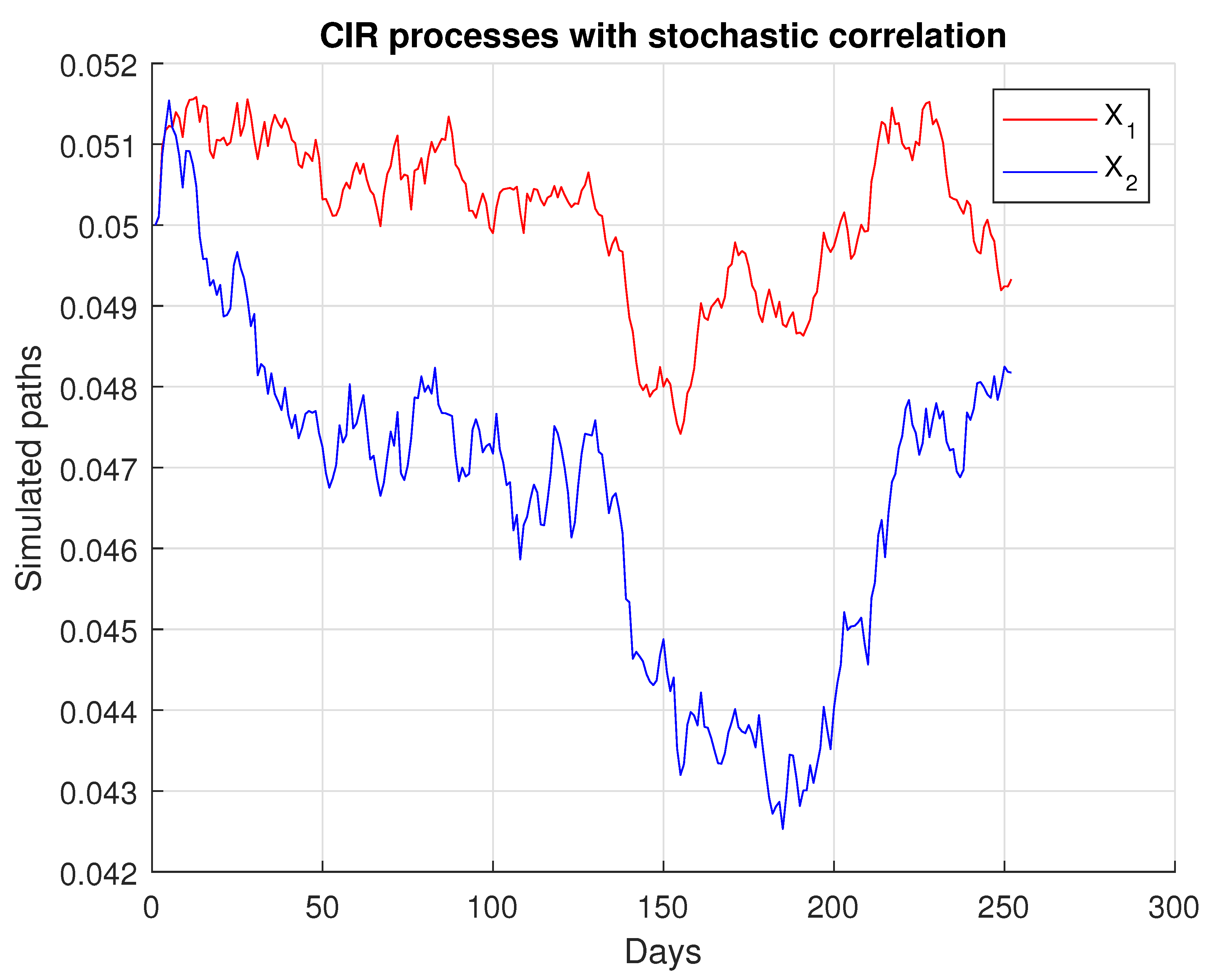
Figure 2.
Instantaneous stochastic correlation coefficient path.
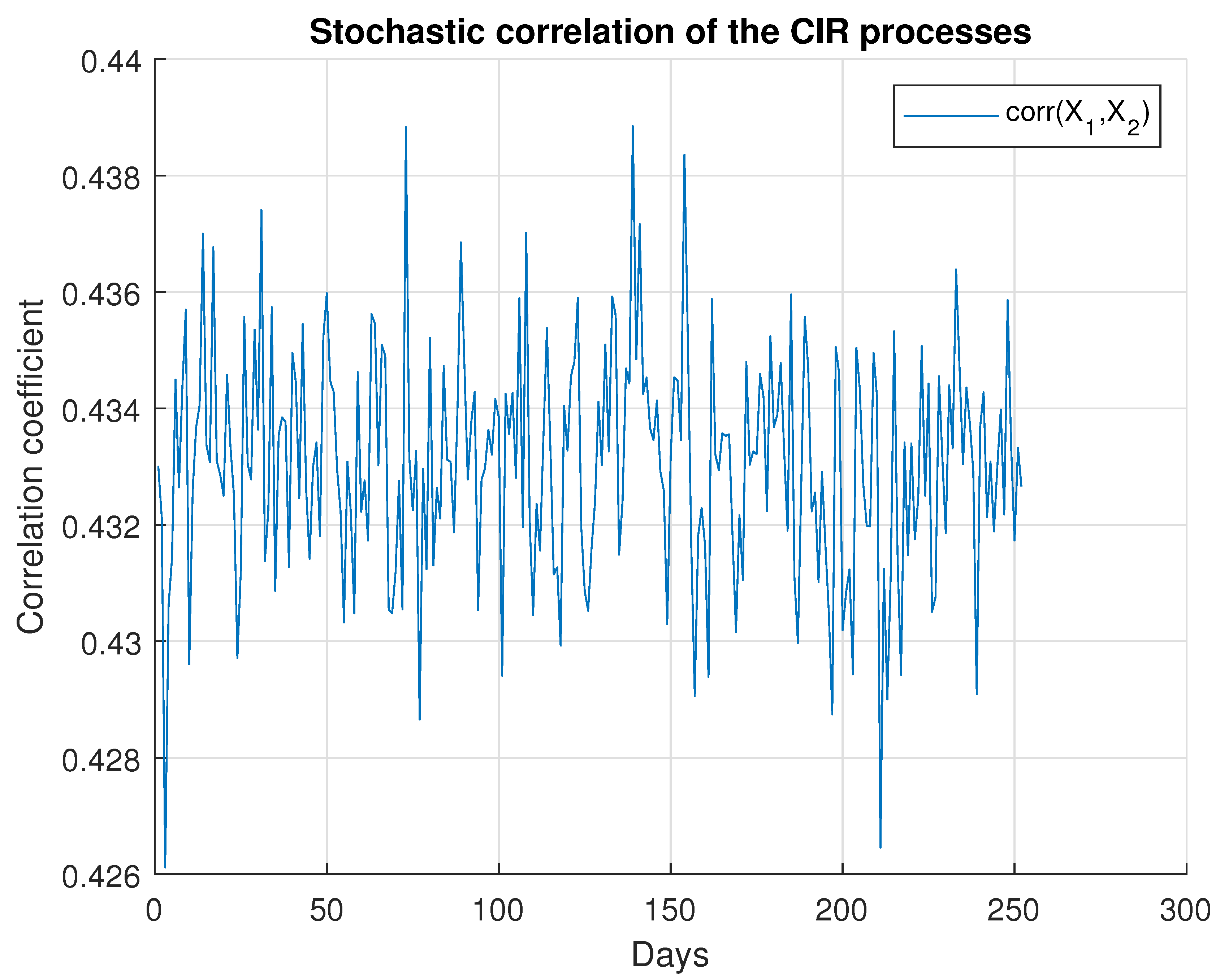
Figure 3.
Stochastic correlation mean for each .
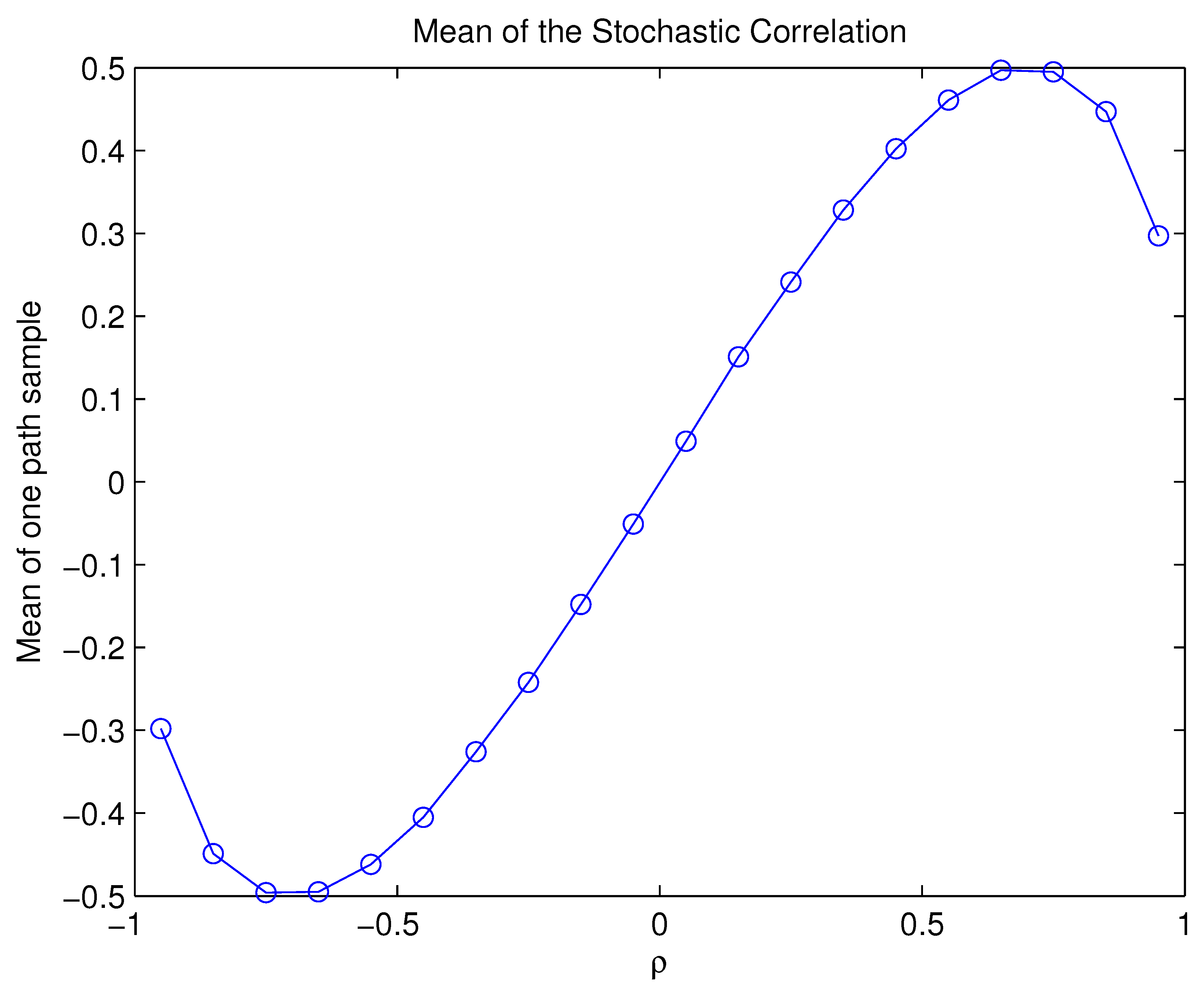
Figure 4.
Stochastic correlation mean for each and .
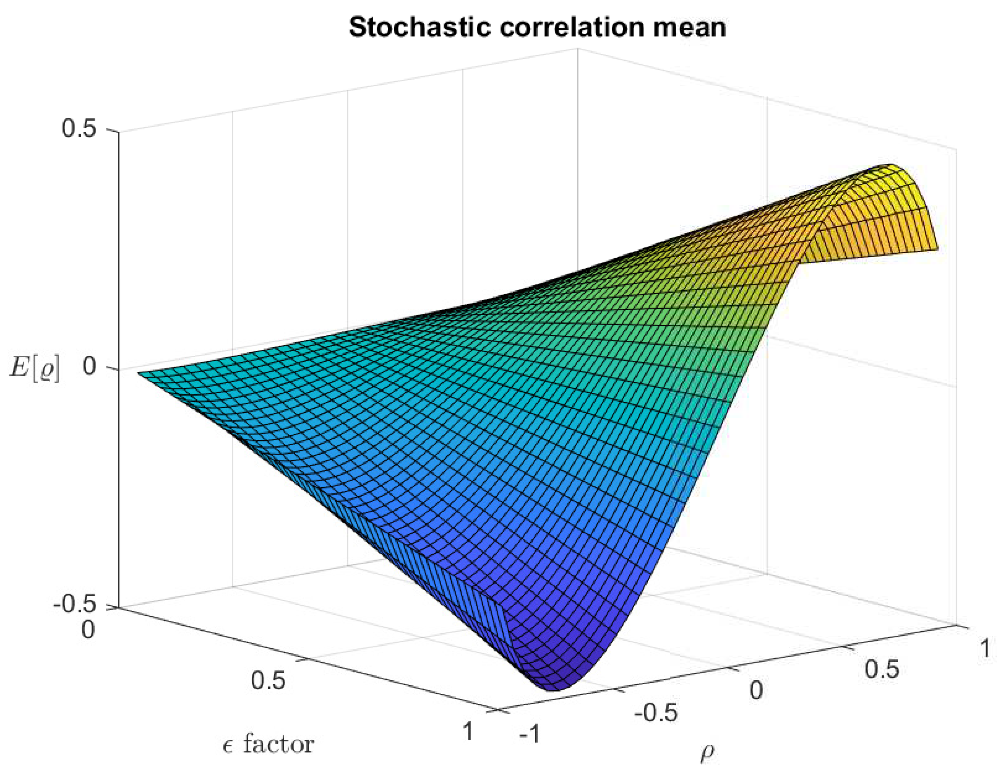
Figure 5.
Stochastic correlation standard deviation for each and .
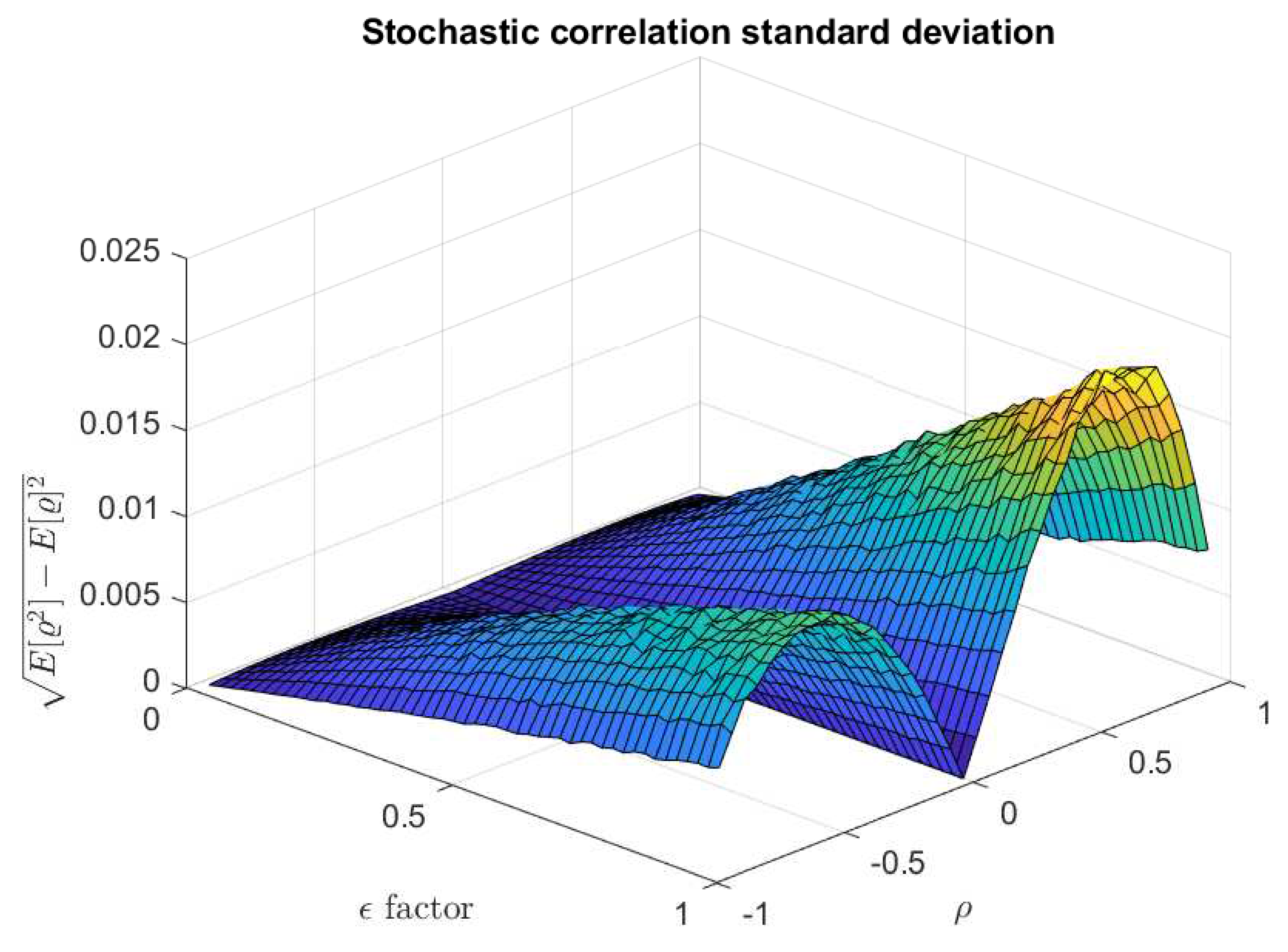
Figure 6.
Probability density functions of .
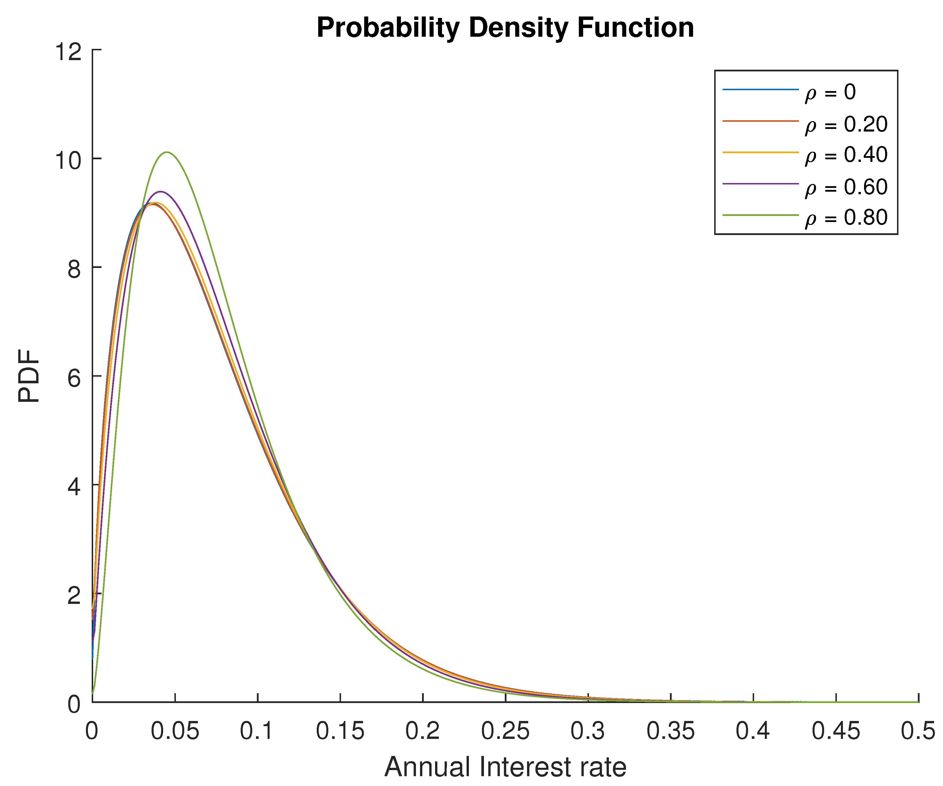
Figure 7.
Probability density functions of .
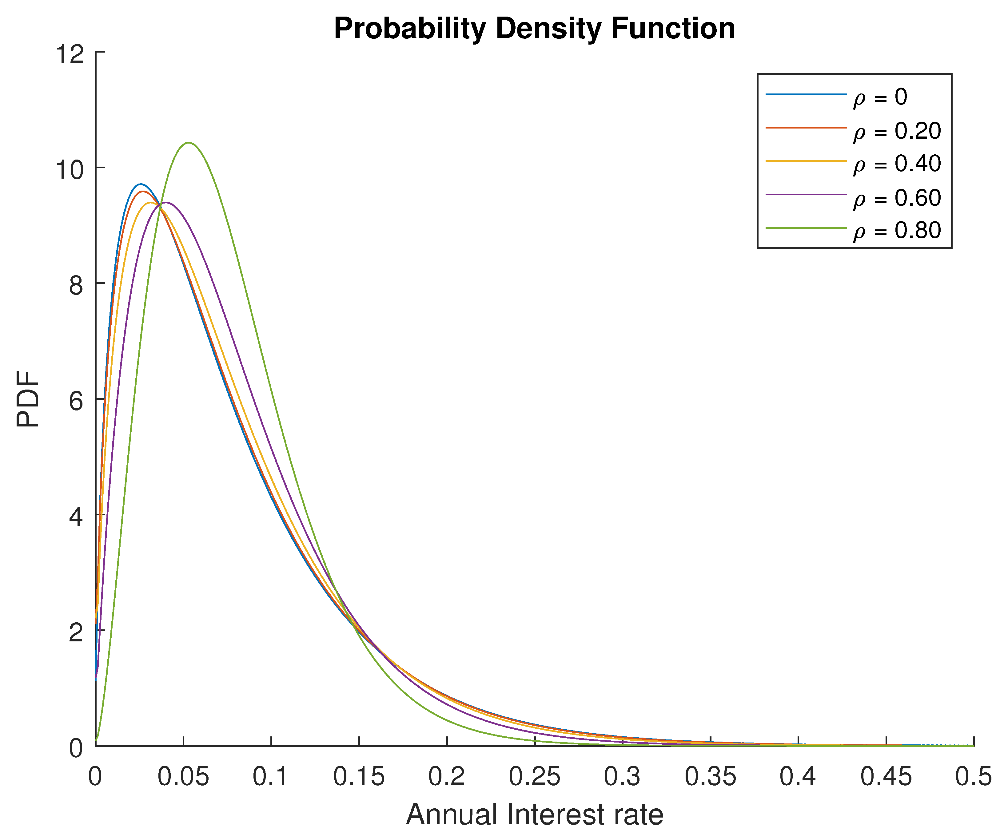
Figure 8.
-parameterized density functions of .
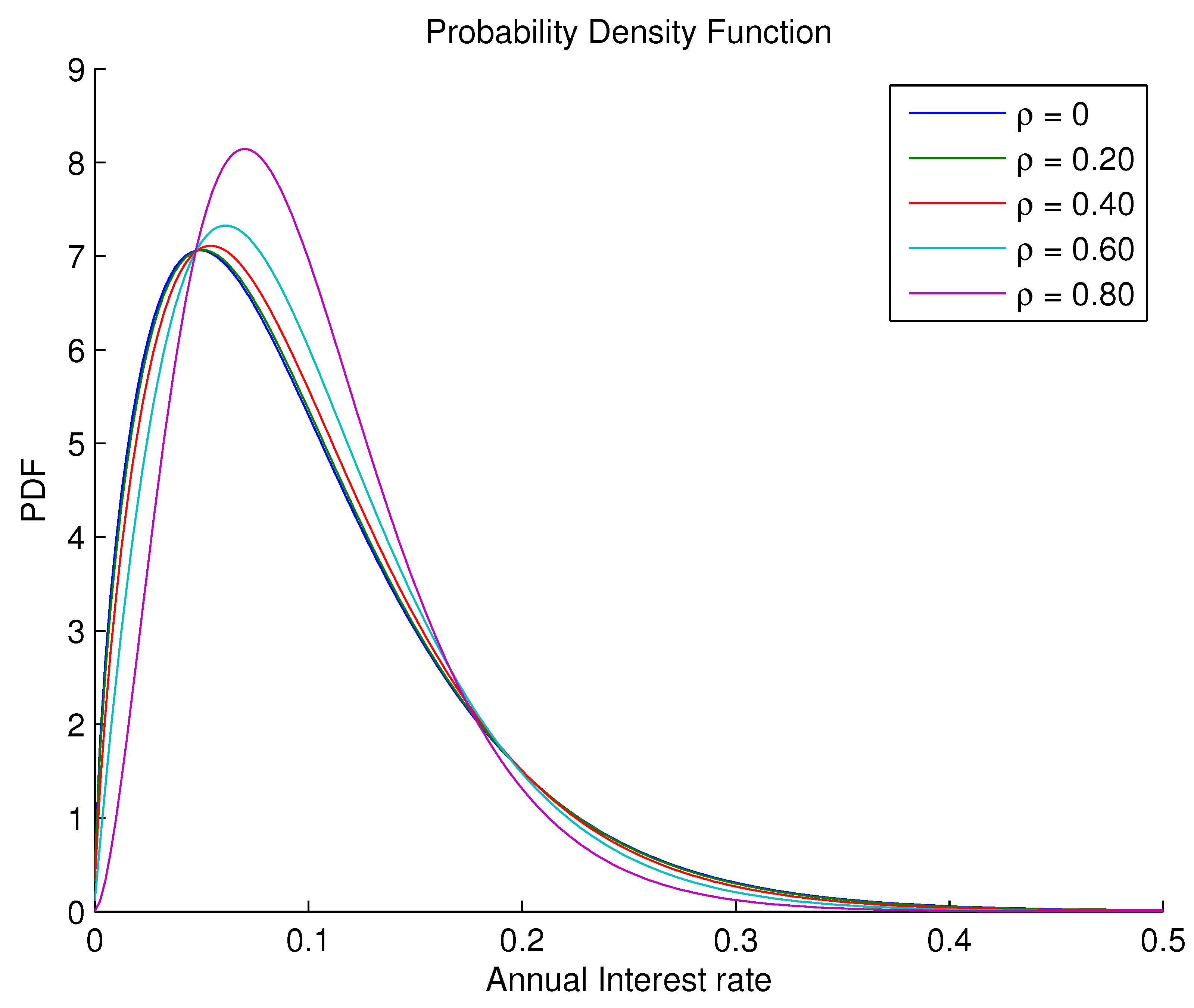
Figure 9.
Evolution of the density function of over time.
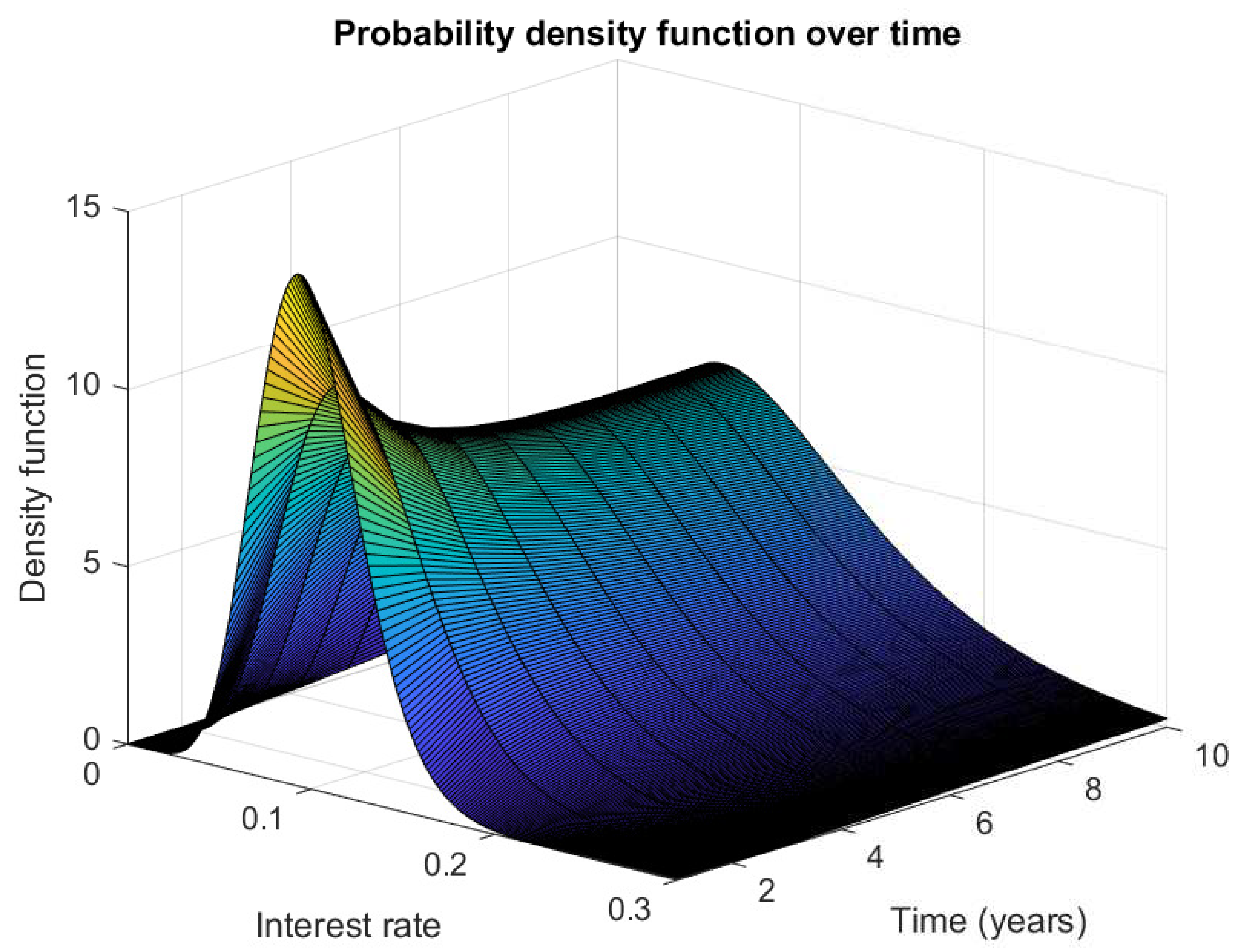
Figure 10.
-parameterized density functions of .
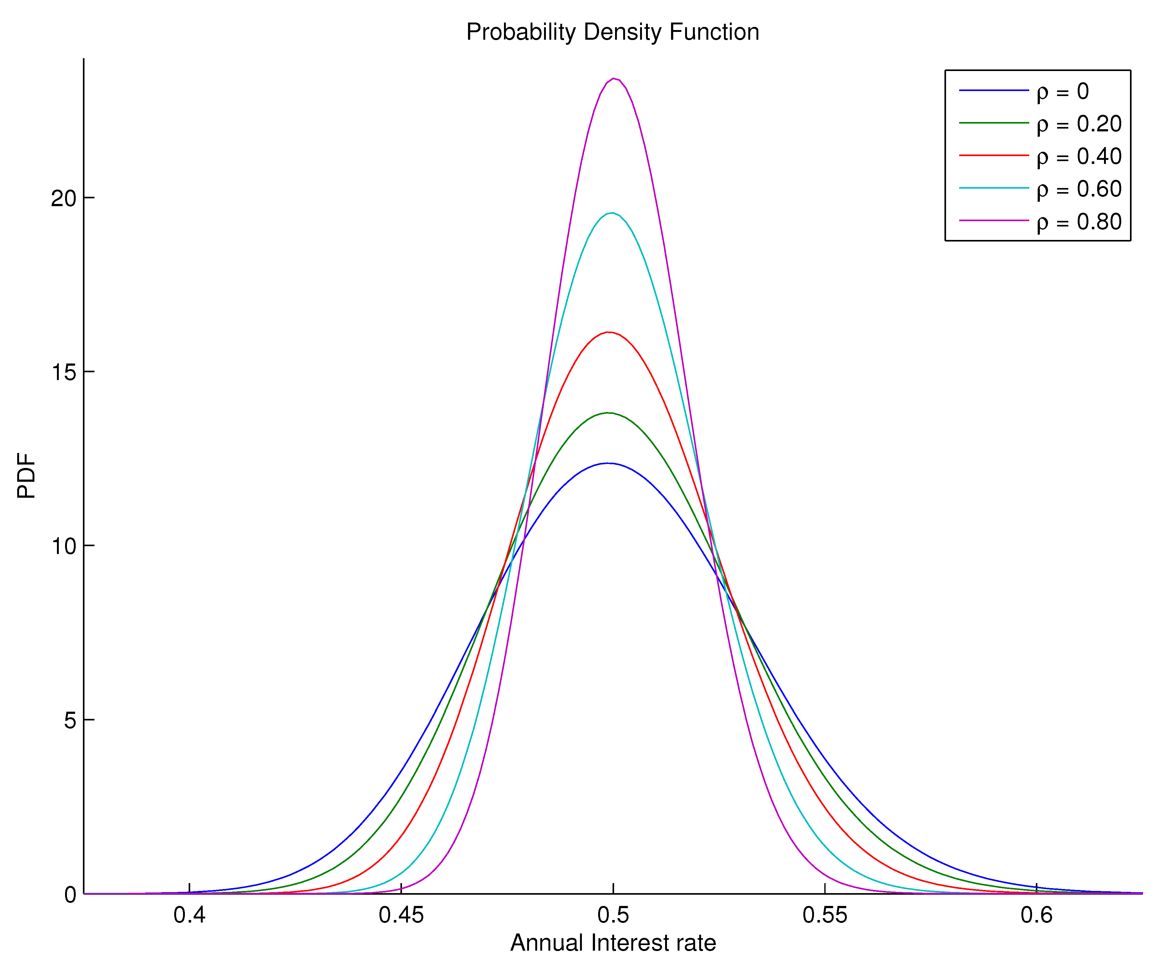
Figure 11.
IDI option prices.
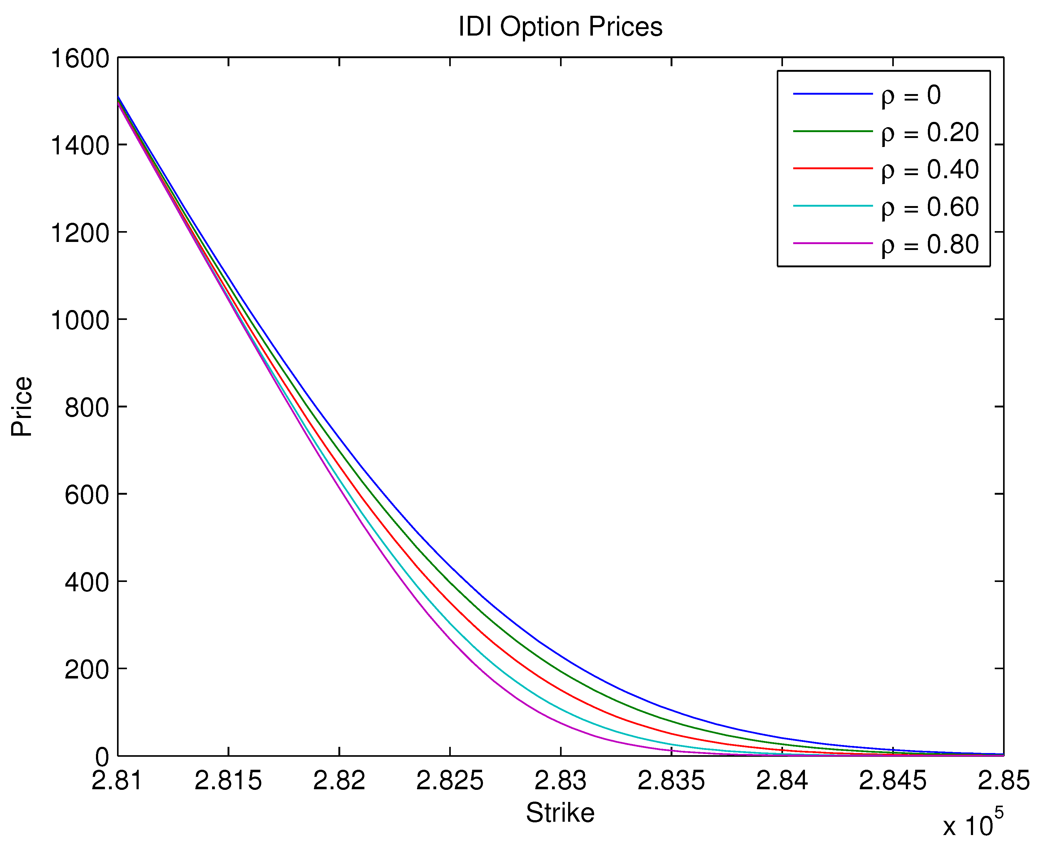

Table 1.
Numerical integral value of the probability density function
| 0 | 0.2 | 0.4 | 0.6 | 0.8 | 0.91 | 0.93 | 0.95 | 0.97 | 0.99 | |
|---|---|---|---|---|---|---|---|---|---|---|
| I | 1.0002 | 1.0005 | 1.0005 | 1.0003 | 1.0000 | 1.0000 | 1.0000 | 1.0000 | 1.0000 | 1.0000 |
Disclaimer/Publisher’s Note: The statements, opinions and data contained in all publications are solely those of the individual author(s) and contributor(s) and not of MDPI and/or the editor(s). MDPI and/or the editor(s) disclaim responsibility for any injury to people or property resulting from any ideas, methods, instructions or products referred to in the content. |
© 2024 by the authors. Licensee MDPI, Basel, Switzerland. This article is an open access article distributed under the terms and conditions of the Creative Commons Attribution (CC BY) license (http://creativecommons.org/licenses/by/4.0/).
Copyright: This open access article is published under a Creative Commons CC BY 4.0 license, which permit the free download, distribution, and reuse, provided that the author and preprint are cited in any reuse.
Submitted:
03 February 2024
Posted:
06 February 2024
You are already at the latest version
Alerts
A peer-reviewed article of this preprint also exists.
This version is not peer-reviewed
Submitted:
03 February 2024
Posted:
06 February 2024
You are already at the latest version
Alerts
Abstract
We introduce a novel stochastically correlated two-factor (i.e., bivariate) diffusion process under the square-root format, for which we obtained, analytically, the corresponding solutions for the conditional moment generating functions and conditional characteristic functions. Such solutions recover verbatim those of the uncorrelated case. We believe that the The aforementioned model encompasses a range of processes similar to that produced by a bivariate square-root process in which entries are correlated in the standard way, i.e., via a constant correlation coefficient. Note that, for the latter, closed-form solutions for the conditional characteristic functions are not available. We focus on the financial scenario of obtaining closed-form expressions for the exact price of a zero-coupon bond and Asian option prices via a Fourier cosine series method.
Keywords:
Subject: Computer Science and Mathematics - Probability and Statistics
1. Introduction
Scalar square-root diffusion processes, also called CIR processes, due to [1], have two properties that are important in applications in finance: (i) they ensure mean reversion of the state variables towards a long run level and (ii) unlike the [2] model, they do not take negative values. The importance of such properties clearly replicates in the multi-dimensional scenario, especially when correlation is allowed among the entries of the process.
In turn, the stochastic models found in finance, especially in interest rate markets, usually assume uncorrelated state variables contradicting both intuition and historical data. In fact, considerable difficulties arise in the pricing procedures when entering with correlation in the model, even when numerical solutions of the corresponding partial differential equations are given by finite difference or finite element methods. Concerning this matter, we quote [3]: “requiring with in the two-factor CIR model would indeed destroy analytical tractability: It would no longer be possible to compute analytically bond prices and rates starting from the short rate factors.” On the other hand, as it is still argued by [3], whenever the correlation plays a more relevant role or when higher precision is needed in the pricing procedure, we need to resort to models that allow for more realistic patterns.
With this in mind, we present a bi-dimensional (two-factor) mean-reversion stochastically correlated process in which entries are produced by two concatenated CIR-type models. Such process is affine according to [4].
We obtained the closed form solution - of exponential format - of the conditional moment generating function and the conditional characteristic function of the density function of the integral of the process governed by the model as well as those of the process itself at final time T. A key point that permitted us to apply the above transforms in the problem of pricing derivatives, particularly with respect to fixed income markets, was devising that the integral of the process - and not the process per se - was the adequate mathematical object to achieve the results.
It is noteworthy that by setting our stochastic correlation to zero we reduce our model to a pair of scalar uncorrelated square-root (CIR) diffusions. We believe that the proposed model encompasses a range of processes similar to that produced by a bivariate CIR process in which entries are correlated in the standard way, i.e., exhibiting a constant correlation coefficient, with the advantage of exhibiting an analytical solution.
We applied our results in the context of the interest rate financial markets where the interest rate process stems from the two-factor stochastically correlated CIR model we present in the paper. We obtained closed-form expressions for the price of a zero-coupon bond and, in the sequel, for the price of the IDI option, an Asian option that commonly appears in the Brazilian fixed-income markets. For the latter case, we used the fast and accurate pricing method based on Fourier series expansions proposed by Fang and Osterlee [5] and applied it to interest rate options in [6].
Via numerical simulations, we showed the (good) behavior of the two-factor process in the face of a certain stochastic correlation condition, under stringent circumstances. Moreover, a result concerning the effect of the sensitivity parameter () on the stochastic correlation coefficient (), and ultimately, the possibility of emulating bivariate CIR processes with constant correlation coefficient, was unveiled. Focusing on the financial scenario, we analyze the impact of the correlation parameter () on the conditional probability density functions associated with the interest rate process - which in turn stems from the two-factor process - obtaining again a good confirmation (non-negativity). Finally, some option price curves are obtained, parameterized by . We also used real data from the financial market in the model design.
The mathematical tools we relied on are the Feynman-Kac formula, the separation of variables approach, the Riccati equations with known explicit solutions and the series expansions proposed by [5].
The rest of this paper is organized as follows: Section 2 presents the stochastically correlated two-factor affine model and its probability background. In Section 3 we derive the expressions of the conditional moment generating function and the conditional characteristic function associated to the model. Section 4 addresses applications to finance, and Section 5 the numerical results.
2. The Model
Let be a filtered space where is a filtration, is a probability measure, and the adapted processes and are independent standard Brownian Motions under (see, e.g., [7]).
We introduce the pair of square-root diffusions, in which the underlying variables are stochastically correlated, as follows. For and initial conditions and ,
and
where and are prescribed random variables and . We have that , and are positive real numbers. Each stochastic process is pulled to a level at a rate with a volatility . We have that and are stochastically correlated processes, where is a Brownian Motion and
is a Itô process.
Hence,
The correlation is specified via the adapted stochastic process
. Note that if , then and we recover the standard uncorrelated case. If we change the specification of to a constant, say, , then and , so becomes a standard Brownian Motion.
The dynamics (1) & (2) also reads
where
and and are independent standard Brownian Motions, as defined at the beginning of the section. Using the specification (5) and after some algebraic manipulation, it follows that is of affine form.
In the above equations, are the speeds of adjustment, are the long-term means, are the volatility factors, is a correlation parameter and is a sensitivity factor - a useful parameter as we shall see in Section 5. Equations (1) and (2) produce Feller processes known in the context of finance as the CIR processes due to [1]. According to [8], the following condition must hold in order to ensure a strong solution for (1) and (2) and to avoid the possibility of negative values of and .
Moreover, we rely on having
In order to conform with the condition above, we benefit from the existence of the sensitivity parameter , setting it as follows.
The comprehensive numerical results of Section 5 assert that the above condition suffices to ensure the good behavior of the correlation process and that the bivariate process x covers a broad range of CIR-type correlated processes.
3. Underpinning Results
The theorems that follow consider the stochastically correlated two-factor process , as given above, relying on the fact that this process is affine. Here ’ stands for the transpose.
The conditional moment generating function and the characteristic function of Theorem 1 will be applied in Section 4 in order to calculate, respectively, the price of a zero coupon bond and the price of an interest rate option, namely, the IDI option. In both cases, the interest rate is given by the additive process (29), stemming from the two-factor process x.
Theorem 1.
The closed-form solution of the conditional characteristic function (resp. conditional moment generating function) associated with the -integral of the two-factor process x with coefficient , namely (resp. ), is given by
where
with
Proof.
We address the proof for the moment generating function case. The proof for the characteristic function case follows closely. So, invoking [4], the moment generating function of a multifactor - say m-dimensional, stochastic differential equation (SDE) of the form
has an exponential affine solution if the above coefficients are of the form
where , , and have adequate dimensions and do not depend on x.
The characteristic function version of the following theorem will be applied in Section 5 in order to calculate the probability density function of the additive process given by Equation (29) exhibited ahead.
Theorem 2.
The closed-form solution of the conditional characteristic function transform associated with the two-factor process x at time T with coefficient , namely, , is given by
where
Proof.
4. Applications to Finance: Fixed Income Markets with Decomposed Nominal Rates
We consider a financial interest rate market underpinned by the short rate stochastic process which stems from the two-factor stochastically correlated (affine) CIR model given by (1)–(4), namely
. We assume that is a risk-neutral probability measure.
Now, recalling the Fisher effect [9] in economics, we have that the nominal short rate can be decomposed into the real interest rate and the inflation expectation. This conforms to our setting, simply particularizing and denoting, for convenience, the real interest rate and the inflation by and respectively.
Under this framework, and relying on Theorem 1, we shall obtain the price of a bond and an interest rate option as follows.
4.1. Bond Pricing
The zero-coupon bond is an interest rate derivative that pays 1 at the expiration date T and no other payment before T. Relying on the seminal work [10], the no-arbitrage price at time of the zero-coupon bond expiring at T is given by
Proposition 1.
Proof.
We may notice that the drift that ultimately appears in dynamic (31) is the short rate process itself, as it ought to be.
As stated by Brigo and Mercurio ([3]), and shown in [11] for example, a two-factor model is capable of explaining up to of the variations in the yield curve. Such a model is needed to provide a realistic evolution of the zero-coupon bond curve. So, we contribute to this, by means of sophisticating the modeling of the term structure of the interest rates via the additive two-factor model given by (1)-(4), (29) and . We also provide a leak concerning the statement made in [3], in which the authors say that “requiring with in the two-factor CIR model would indeed destroy analytical tractability: It would no longer be possible to compute analytically bond prices and rates starting from the short rate factors.” Indeed, we have shown that bond prices are analytically tractable under the two-factor correlated CIR model mentioned above.
5. Numerical Results
In this section, we discuss some issues of the stochastic correlated square-root diffusion process given by Equations(1)–(4). In Section 5.1, we study the model’s behavior in the face of condition given by the inequality (9) - which involves the stochastic correlation coefficient . In (Section 5.2) we study the variation of the stochastic correlation coefficient in time and in the probability space for fixed parameters and . In the sequel we let these parameters vary.
Via Fourier series, we proceed to present the conditional probability density function of the integral of the short rate process R - the weighted sum of the components of the two-factor CIR model (1)–(4) (see Equation (29)). The conditional probability density function is equally provided for R at terminal date T. Such sort of conditional density functions are the cornerstones for obtaining the price of financial derivative contracts. We shall see that, in the long run especially, the correlation parameter plays a sensitive role in the volatility of the zero coupon bond, and therefore on the prices of interest rate derivatives in general. In the sequel, we obtain the price of the IDI option (Section 5.4).
Nonetheless, the important stochastic correlation analysis will be carried out varying in the whole range given by (33). Our dynamic is as given by Equations (1)–(4) with , , , , , , year, and initial condition and . We also set . We benefit from the existence of the sensitivity parameter , setting it equal to the maximal value of the range given by (10), i.e.,
This maximum value will hold throughout the section. Nonetheless, the important stochastic correlation analysis will be carried out varying in the whole range given by (10).
5.1. The Stochastic Correlation Condition (9) is Mild, at Least at a Certain Niche
To verify if the stochastic correlation coefficient performs according to condition (9), we produced 100.000 path simulations of the stochastic correlated CIR process with time discretization years and period of one year, using the simple Euler scheme as given in [12].
Firstly, we used [13], which provided us with parameter estimates based on real-world financial data. There, the authors used a three-factor uncorrelated CIR process to model zero-coupon bonds. We tested all three possible combinations of the parameters presented in Table 2 of the referenced paper, not finding a rate over concerning pointwise violations of the stochastic correlation condition (9) throughout , for a variety of values of .
In order to test a more restrictive scenario, we set , and for and . While agreeing with condition (8), the setup above enforces the model to violate the stochastic correlation condition. But still, at the beginning, no violation of this condition occurred for a variety of values of . Violations start appearing when breaches . Nevertheless, its rate did not surpass for a reasonable broad range of , typically up to . Whence, this shows that condition (9) is in fact mild, at least for prescribed as in (33). Also, we noticed that the violation rate decreased as we lowered the correlation parameter .
5.2. Hand-Conducting the Model via
Figure 2 shows a sample path of the stochastic correlation coefficient as given by (5). It suggests that has little variation over time. Also, from the simulations we could infer that, for any , of the sample paths lay within the range of .
We may therefore infer that our model can be a good approximation to correlated CIR models with constant correlation coefficient, with the advantage of exhibiting an analytical pricing solution.
Now, for each and for prescribed by the relation (33), Figure 3 exhibits the mean value over time of a corresponding sample path of the stochastic correlation coefficient. Since does not vary much either in time or in space, we shall rename this mean value as the operation point of the stochastic correlation coefficient, for each .
As we can see in Figure 3, this operation point covers the interval , which is not very broad but still a reasonable range as we vary . Alternatively, we can depart from the maximum value of given by inequality (33) to an arbitrary value in a certain confidence interval, so we can hand-conduct the curve of operation points to another more desired range.
Figure 4 shows the stochastic correlation mean surface for varying in the range given by (10) and Figure 5 shows the corresponding standard deviation. These two graphs illustrate important findings. Firstly, for every in ,
- the correlation mean vanishes when (see Figure 4).
- the correlation stochasticity also vanishes when ,(see Figure 5).
In addition, the model recast the specific case of uncorrelated CIR model when either or , for any given parameter values.
Secondly, while not near the degenerated zero value, indeed introduces a correlation between the entries of the process generated by the model, whose intensity varies considerably as we hand-conduct it within the range established in (10).
These qualities underscore the model’s versatility in capturing a range of behaviors, including scenarios that are essential for theoretical analysis and practical applications.
5.3. Conditional Probability Density Functions of the Short Rate Process
We use the COS method ([5]) to recover the conditional probability density function of the -integral of the short rate process R. The approximation of f is given by the following Fourier-cosine series
for a given N. If f, with domain in , is a probability density function of X, then
where is the characteristic function of X, that is
which approximates
We set for the sake of truncating the series. The parameters are given by Equation (35) which in turn is calculated by means of the characteristic function (12). The same procedure holds for obtaining the conditional probability density function of the short rate process itself at terminal date T, in which case the characteristic function is given by Equation (21).
Figure 8 shows the -conditional probability density functions of versus the correlation parameter . High correlation, thin right tail. The lower the correlation, the more positively skewed the density is. We may also infer from the figure that the stochastic correlated CIR processes preclude negative values concerning the additive process R, so preserving the property of the single and two-factor uncorrelated square-root diffusion process (see Figure 9 for the surface of the density over time). Table 1 confirms this statement, presenting the cumulative area under the probability density function for different values of .
Figure 10, in turn, shows the -conditional probability density functions of the -integral of R versus . The lower the correlation parameter, the higher its dispersion. It is worth noticing how sensitive the shape of this density function is as we vary the parameter , which suggests that correlation is a subject matter that cannot be neglected. The above probability density function is used for calculating the price of the IDI option.
5.4. Pricing the IDI Option
As stated by [5], the price of a European option can be approximated by
where the coefficients are given by (35) and
where refers to the payoff of the financial contract.
We assume an interest rate market with underlying probability space equipped with a filtration where is the risk neutral measure.
An overnight interest rate is the average of the interbank rate of a one-day period, calculated daily and expressed as the effective rate per annum. So, the Interbank Deposit Rate Index (IDI) accumulates discretely, according to
where j denotes the end of day and assigns the corresponding overnight rate.
If we approximate the continuously overnight rate by the instantaneous continuously compounding interest rate, i.e., , the index can be represented by the following continuous compounding expression
Given non-negative interest rates, the index is a non-decreasing function of .
A European call option is a contract that gives the owner the right, but not the obligation, to buy a specified amount of an underlying security at a specified price and at a specified time. The payoff of the IDI call option maturing at T is
where K is the strike price. Therefore, the price at time t of this option is
In order to price the IDI option we compute the characteristic function of the path-dependent integral of the interest rate - namely - which in turn will give us the values of associated to the model. So, the price of the IDI option can be calculated via the COS method. Equation (43) gives the payoff of the IDI call option so that the coefficients are given by
and
The coefficients are calculated with (35) by using the characteristic function given by Theorem 1.
Figure 11 gives us the IDI option prices with year and the initial value of the IDI given by . We note that the lower the correlation parameter, the higher the option prices, notably for at-the-money options where the low-correlated options can reach four times the price of the highly correlated contract. This is due to the effect of reducing the uncertainty implied by the probability distribution shown in Figure 10. Again, this shows that correlation is a subject that cannot be neglected.
6. Conclusion
We unveiled a bivariate model under the square-root diffusion (CIR) format equipped with a stochastic correlation coefficient for which we have obtained the analytical solution of the conditional moment generating function and the conditional characteristic function of the related diffusion process that stems from that model. Inter alia, this immediately facilitates obtaining closed-form expressions for the prices of a variety of interest rate derivatives. Remind that obtaining analytical results is a quality not achievable in the case of bivariate CIR models with constant correlation coefficient.
Varying a certain parameter () serves to hand-conduct the model’s design changing the strength of correlation between the entries of the process. Figure 4 and Figure 5 illustrate this well. Also, by setting equal to zero, we recover the two-factor uncorrelated square-root diffusion model.
These qualities - the analycal results in conjunction with stablishing correlations and recevering the uncorrelated CIR case - underscore the model’s versatility in capturing a range of behaviors that include scenarios that are essential for theoretical analysis and practical applications.
In addition, the simulations herein strongly suggest that the model precludes negative values, whence preserving the quality of the single and two-factor uncorrelated CIR process.
Finally, subscribed to this model, we obtained the closed-form expressions of the exact price of a zero coupon bond and a certain Asian option - the so-called IDI option.
Conflicts of Interest
The authors declare no conflicts of interest.
References
- Cox, J.C.; Ingersoll, J.; Ross, S. A Theory of the Term Structure of Interest Rates. Econometrica 1986, 53, 385–407. [Google Scholar] [CrossRef]
- Vasicek, O. An Equilibrium Characterization of the Term Structure. Journal of Financial Economics 1977, 5, 177–188. [Google Scholar] [CrossRef]
- Brigo, D.; Mercurio, F. Interest Rate Models - Theory and Practice; Springer Finance, Springer: Berlin, 2006. [Google Scholar]
- Duffie, D.; Singleton, K.J. Credit risk: Pricing, measurement, and management; Princeton University Press, 2003.
- Fang, F.; Oosterlee, C.W. A Novel Pricing Method for European Options Based on Fourier-Cosine Series Expansions. SIAM Journal on Scientific Computing 2008, 31(2), 826–848. [Google Scholar] [CrossRef]
- da Silva, A.J.; Baczynski, J.; Bragança, J.F.S. Path-Dependent Interest Rate Option Pricing with Jumps and Stochastic Intensities. Lecture Notes in Computer Science 2019, 11540, 710–716. [Google Scholar] [CrossRef]
- Protter, P.E. Stochastic Integration and Differential Equations; Springer: Berlin, 2005. [Google Scholar] [CrossRef]
- Bertini, L.; Passalacqua, L. Modelling Interest Rates by Correlated Multi-Factor CIR-Like Processes. Working Paper 2008, 10. [Google Scholar] [CrossRef]
- Fisher, I. The Theory of Interest; Macmillan, 1930.
- Harrison, M.; Pliska, S. Martingales and stochastic integrals in the theory of continuous trading. Stochastic Processes and their Applications 1981, 11, 215–260. [Google Scholar] [CrossRef]
- Jamshidian, F.; Zhu, Y. Scenario Simulation: Theory and Methodology. Finance and Stochastics 1997, I, 43–67. [Google Scholar] [CrossRef]
- Glasserman, P. Monte Carlo Methods in Financial Engineering; Applications of mathematics: Stochastic modelling and applied probability, Springer, 2004. [Google Scholar]
- Almeida, C.; Vicente, J.V. Are interest rate options important for the assessment of interest rate risk? Journal of Banking and Finance 2009, 33, 1376–1387. [Google Scholar] [CrossRef]
Figure 1.
Stochastic correlated paths.
Figure 2.
Instantaneous stochastic correlation coefficient path.
Figure 3.
Stochastic correlation mean for each .
Figure 4.
Stochastic correlation mean for each and .
Figure 5.
Stochastic correlation standard deviation for each and .
Figure 6.
Probability density functions of .
Figure 7.
Probability density functions of .
Figure 8.
-parameterized density functions of .
Figure 9.
Evolution of the density function of over time.
Figure 10.
-parameterized density functions of .
Figure 11.
IDI option prices.
Table 1.
Numerical integral value of the probability density function
| 0 | 0.2 | 0.4 | 0.6 | 0.8 | 0.91 | 0.93 | 0.95 | 0.97 | 0.99 | |
|---|---|---|---|---|---|---|---|---|---|---|
| I | 1.0002 | 1.0005 | 1.0005 | 1.0003 | 1.0000 | 1.0000 | 1.0000 | 1.0000 | 1.0000 | 1.0000 |
Disclaimer/Publisher’s Note: The statements, opinions and data contained in all publications are solely those of the individual author(s) and contributor(s) and not of MDPI and/or the editor(s). MDPI and/or the editor(s) disclaim responsibility for any injury to people or property resulting from any ideas, methods, instructions or products referred to in the content. |
© 2024 by the authors. Licensee MDPI, Basel, Switzerland. This article is an open access article distributed under the terms and conditions of the Creative Commons Attribution (CC BY) license (http://creativecommons.org/licenses/by/4.0/).
Copyright: This open access article is published under a Creative Commons CC BY 4.0 license, which permit the free download, distribution, and reuse, provided that the author and preprint are cited in any reuse.
Analytically Computing the Moments of a Conic Combination of Independent Noncentral Chi-Square Random Variables and Its Application for the Extended Cox–Ingersoll–Ross Process with Time-Varying Dimension
Sanae Rujivan
et al.
Mathematics,
2023
An Empirical Investigation to the “Skew” Phenomenon in Stock Index Markets: Evidence from the Nikkei 225 and Others
Yizhou Bai
et al.
Sustainability,
2019
Qualitatively Stable Schemes for the Black–Scholes Equation
Mohammad Mehdizadeh Khalsaraei
et al.
Fractal Fract,
2023


MDPI Initiatives
Important Links
© 2024 MDPI (Basel, Switzerland) unless otherwise stated