On Adaptive Identification of Interconnected Systems

Preprint

Article

On Adaptive Identification of Interconnected Systems

Altmetrics

Downloads

100

Views

Comments

Nikolay Karabutov^*

This version is not peer-reviewed

This preprints belongs to the Topic

Advanced Operation, Control, and Planning of Intelligent Energy Systems

Submitted:

02 February 2024

Posted:

07 February 2024

You are already at the latest version

Alerts

Abstract

. Interconnected control systems (ICS) widely apply to various technical systems. ICS has a complex description. Therefore, simplified models use, which the specifics of an object do not always reflect. So, the problem of synthesizing mathematical models is topical. The work purpose is to develop an approach to obtaining models in conditions of incomplete a priori information. We use an adaptive approach. As examples, two-channel systems (TCS) with cross-links and identical channels consider, and a method for mathematical model design. We consider the system with asymmetric cross-links and evaluate their impact on properties of an adaptive identification system. Approach proposed to assessing the TCS identifiability with cross-links. The excitation constancy influence on TСS parameter estimates is studied. A generalization of the proposed approach is given for an interconnected system.

Keywords:

Subject: Computer Science and Mathematics - Mathematics

1. Introduction

Interconnected systems (ICS) used [1,2,3,4,5] to control actuators for robots and manipulators [6,7], and various technical systems [8,9]. ICS identification methods based on an adaptive approach [10], a black box concept for non-stationary multi-connected systems with uncertainty [11]. Adaptive algorithms of decentralized robust control with a reference model are proposed for ICS with a time delay [12]. The identifiability issues considering for a closed interconnected stochastic system in [13]. The system decomposition proposes into subsystems. The identifiability considers as system individual elements and individual closed circuits. Convergence sufficient conditions got almost certainly for parameter estimates. A high-modulus normalized adaptive lattice algorithm proposes for multichannel filtering in [14].

In [15], an algorithm presents to identify transfer function models for 2-D spatially interconnected systems which are semi-causal both in open and closed-loop form using neural network. In [16], a decentralized robust adaptive stabilization system considers with output feedback. adaptive nonlinear damping and a robust adaptive observer are the base for controlling laws. In [17,18], there get similar results. In [19], the identification method presents for a spatially interconnected system in a rational form.

Adaptive control of large-scale systems consisting for arbitrary of subsystems with unknown parameters, nonlinearities and limited perturbations is considered in [20]. Topological structural identification [21] considers for large-scale dynamic systems based on a small dataset. In [22], the approach proposes to the blind identification of a two-channel systems. The proposed approach bases on the data analysis in the frequency domain. Problem analysis of blind multichannel identification and some modern adaptive algorithms present in [23]. The review [24] analyzed some modern approaches based on the identification problem (IP) decomposition for systems with multiple inputs /one output (MISOS). The identification of stationary linear MISOS discusses in [13,25,26]. Correlation analysis [25] uses for the ICS identification in the frequency domain.

Transfer functions and the state space Models are the basis for analyzing processes in ICS. Adaptive procedures are used to synthesize control algorithms. Adaptive control algorithms apply under the perturbations and unmodeled dynamics action. Explain this IP state (i) incomplete information about the state and parameters of the system and (ii) the accounting complexity of relationships in the system. The identification of ICS parameters base on statistical procedures, frequency methods and neural network technologies. Apply of adaptive identification methods (AIM) study in some works. AIM use to the tuning (identification) control parameters. Parametric uncertainties that arise in this case compensate by the choice of a control algorithm. The Identification of two-channel systems has not been studied.

We propose the approach to the ICS adaptive identification based on the use of measurement results. First, two-channel systems (TCS) with cross-links (CL) are considered. The approach proposes to the TCS identifiability under various assumptions about LC. Identifiability estimates have obtained. The adaptive system stability proves. We propose the approach to ICS identification.

2. Two-channel systems

2.1. Problem Setting

Consider TCS with CL. We believe that elements in channels are identical. Transfer functions are the basis of TCS analysis [27]. The TCS description in the state space is a more adequate representation in identification problems. Let TCS have

n

vertical layers.

(i): the first layer

\begin{array}{l} {\begin{cases} {\dot{X}}_{11} = A_{1} X_{11} + B_{1} e_{11} = A_{1} X_{11} + B_{1} v_{11}, \\ y_{11} = C_{1}^{T} X_{11}, \end{cases} \\ {\begin{cases} {\dot{X}}_{21} = A_{1} X_{21} + B_{1} e_{21} = A_{1} X_{21} + B_{1} v_{21}, \\ y_{21} = C_{1}^{T} X_{21}, \end{cases} \end{array}

(1)

(ii): $k$ -layer ( $1 < k \leq n$ )

\begin{array}{l} {\begin{cases} {\dot{X}}_{1, k} = A_{k} X_{1, k} + B_{k} u_{1, k}, \\ y_{1, k} = C_{k}^{T} X_{1, k}, \\ u_{1, k} = y_{1, k - 1} + v_{1, k - 1}, \\ v_{1, k - 1} = d_{k - 1} (y_{2, k - 1} + d_{k - 2} v_{2, k - 1}), \end{cases} \\ {\begin{cases} {\dot{X}}_{2, k} = A_{k} X_{2, k} + B_{k} u_{2, k}, \\ y_{2, k} = C_{k}^{T} X_{1, k}, \\ u_{2, k} = y_{2, k - 1} + v_{2, k - 1}, \\ v_{2, k - 1} = d_{k - 1} (y_{1, k - 1} + d_{k - 2} v_{1, k - 1}), \end{cases} \end{array}

(2)

where

v_{11} = g_{1} - y_{1, n}, v_{21} = g_{2} - y_{2, n}

v_{i, k - 1}

is i-channel CL output,

i = 1, 2

;

X_{i k} \in ℝ^{q}

is the state vector of the

k

layer of the

i

channel,

A_{k} \in ℝ^{q_{k} \times q_{k}}

C_{k} \in ℝ^{q_{k}}

B_{k} \in ℝ^{q_{k}}

y_{i, k} \in ℝ

is output

k

layer of the

i

channel;

v_{i, k - 1}

is CL output;

g_{i} (t) \in ℝ

is input (upsetting control) the system.

A_{k}

is Hurwitz matrix.

d_{k - 1}

is an operator. Tasks solved by TCS determine the

d_{k - 1}

type.

d_{k - 1}

can be a constant, a nonlinear function, or a differential operator.

Information set

{II}_{o} = {g_{i} (t), y_{i, k} (t) \forall (i = 1; 2) & (k = \bar{1, n}), t \in J = [t_{0}, t_{e}]}

(3)

where

J

time interval.

The structure of the TCS model coincides with (1), (2). Let

{\hat{y}}_{i, k} \in ℝ

i = 1, ​ 2; k = \bar{1, n}

is the output model.

Task: design algorithms for tuning model parameters to

\lim_{t \to \infty} | {\hat{y}}_{i, k} - y_{i, k} | \leq δ_{i, k}

(4)

where

δ_{i, k} \geq 0

is a set value.

2.2. About TCS structural aspects

The system (1), (2) identification depends on the evaluating possibility of its parameters.

Introduce the model for (1)

\begin{array}{l} {\begin{cases} {\dot{\hat{X}}}_{11} = K_{1} ({\hat{X}}_{11} - X_{11}) + {\hat{A}}_{1} X_{11} + {\hat{B}}_{1} v_{11}, \\ {\hat{y}}_{11} = C_{1}^{T} {\hat{X}}_{11}, \end{cases} \\ {\begin{cases} {\dot{\hat{X}}}_{21} = K_{1} ({\hat{X}}_{21} - X_{21}) + {\hat{A}}_{1} {\hat{X}}_{21} + {\hat{B}}_{1} v_{21}, \\ {\hat{y}}_{21} = C_{1}^{T} X_{21}, \end{cases} \end{array}

(5)

where

K_{1} \in ℝ^{q_{1} \times q_{1}}

is stable matrix (reference model);

{\hat{A}}_{1} \in ℝ^{q_{1} \times q_{1}}

{\hat{B}}_{1} \in ℝ^{q_{1}}

are matrixes (5),

{\hat{X}}_{i, 1}

is model state vector.

Let

E_{11} ≜ {\hat{X}}_{11} - X_{11}

E_{21} ≜ {\hat{X}}_{21} - X_{21}

. Then for the first layer

\begin{array}{l} {\dot{E}}_{11} = K_{1} E_{11} + Δ A_{1} X_{11} + Δ B_{1} v_{11}, \\ {\dot{E}}_{21} = K_{1} E_{21} + Δ {\hat{A}}_{1} {\hat{X}}_{21} + Δ {\hat{B}}_{1} v_{21}, \end{array}

(6)

where

Δ A_{1} ≜ {\hat{A}}_{1} - A_{1}, Δ B_{1} ≜ {\hat{B}}_{1} - B_{1}

are matrices of parametric residuals.

Similarly, we obtain the error equations for the remaining layers TCS

\begin{array}{l} {\dot{E}}_{1, k} = K_{k} E_{1, k} + Δ A_{k} X_{1, k} + Δ B_{k} u_{1, k}, \\ {\dot{E}}_{2 k} = K_{k} E_{2, k} + Δ {\hat{A}}_{k} {\hat{X}}_{2, k} + Δ {\hat{B}}_{k} u_{2, k} . \end{array}

(7)

Let the input

g_{i} (t)

i = 1; 2

satisfy the constant excitation (CE) condition

E C_{{\underline{α}}_{i}, {\bar{α}}_{i}} : {\underline{α}}_{i} \leq g_{i}^{2} (t) \leq {\bar{α}}_{i} \forall t \in [t_{0}, t_{0} + T],

(8)

where

{\underline{α}}_{i}, {\bar{α}}_{i}

are positive numbers,

T > 0

Designations:

(1) if condition (8) is true, then we write

g_{i} (t) \in E C_{{\underline{α}}_{i}, {\bar{α}}_{i}}

;

(2) if condition (8) is not satisfied, then

g_{i} (t) \notin E C_{{\underline{α}}_{i}, {\bar{α}}_{i}}

Theorem 1.

Let 1)

g_{i} (t) \in E C_{{\underline{α}}_{i}, {\bar{α}}_{i}}

, where

({\underline{α}}_{i}, {\bar{α}}_{i}) > 0

; 2) the system (5) is stable and detectable; 3)

K_{1} \in ℝ^{q_{1} \times q_{1}}

is Hurwitz matrix; 4)

v_{i 1} (t) \in E C_{{\underline{σ}}_{i 1}, {\bar{σ}}_{i 1}}

, where

{\underline{σ}}_{i 1} > 0, {\bar{σ}}_{i 1} > 0

i = 1, 2

; 5)

X_{i 1} (t) \in E C_{{\underline{α}}_{X_{i 1}}, {\bar{α}}_{X_{i 1}}}

, where

({\underline{α}}_{X_{i 1}}, {\bar{α}}_{X_{i 1}}) > 0

. Then the system (5) is identifiable if

π_{12} {‖ Δ A_{1} ‖}^{2} + 0.5 υ_{12} {‖ Δ B_{1} ‖}^{2} \leq (λ - 0.5) V_{1}

(9)

where

λ_{1} > 0.5

π_{12} = 2 \max ({\bar{α}}_{X_{11}}, {\bar{α}}_{X_{12}})

υ_{12} = {\bar{σ}}_{11} + {\bar{σ}}_{21}

{‖ Δ A_{1} ‖}^{2} = tr (Δ A_{1}^{T} Δ A_{1})

tr

is spur of matrix,

V_{1} (t) = 0.5 E_{11}^{T} (t) R_{1} E_{11} (t) + 0.5 E_{21}^{T} (t) R_{1} E_{21} (t)

R_{1} = R_{1}^{T} > 0

is symmetric matrix.

The theorem 1 proof gives in the appendix A.

Definition 1.

If condition (9) satisfies, then the system (5) is

P I_{1, X}

-identifiable on a set of state variables.

The subsystem layer (1) identifiability depends on properties of the TCS output.

Consider the system (7) and the Lyapunov function (LF)

V_{k} (t) = 0.5 E_{1, k}^{T} (t) R_{k} E_{1, k} (t) + 0.5 E_{2, k}^{T} (t) R_{k} E_{2, k} (t) .

(10)

Theorem 2.

Let (i)

K_{k} \in ℝ^{q_{k} \times q_{k}}

is Hurwitz matrix; (ii)

{‖ X_{1, k} ‖}^{2} \in E C_{{\underline{α}}_{X_{1, k}}, {\bar{α}}_{X_{1, k}}}

{‖ X_{2, k} ‖}^{2} \in E C_{{\underline{α}}_{X_{2, k}}, {\bar{α}}_{X_{2, k}}}

;

π_{k} = \max ({\bar{α}}_{X_{1, k}}, {\bar{α}}_{X_{2, k}})

y_{2 k - 1} \in E C_{{\underline{α}}_{y_{2, k - 1}}, {\bar{α}}_{y_{2, k - 1}}}

; (iii) the system (5) is

P I_{1, X}

-identifiable; (iv) the system (7) is stable and; (v)

v_{2, k - 1}^{2} \in E C_{{\underline{α}}_{v_{2, k - 1}}, {\bar{α}}_{v_{2, k - 1}}}

; (vi) the

d_{k - 1}

operator is constant:

d_{k} \leq ω_{k} \leq ω

, where

ω

is some number; 6)

λ_{k} \geq 0.5

. Then the system (7) is

P I_{k, X}

-identifiable if

. 0.5 π_{k, i} {‖ Δ A_{k} ‖}^{2} + 0.5 {‖ Δ B_{k} ‖}^{2} ({\tilde{\bar{α}}}_{k} + 2 ω^{2} ({\tilde{\bar{α}}}_{k} + 2 ω^{2} β_{k})) \leq (λ_{k} - 0.5) V_{k}

(11)

where

π_{k, i} = 2 \max ({\bar{α}}_{X_{1, k}}, {\bar{α}}_{X_{2, k}})

{\tilde{\bar{α}}}_{k} = 2 \max ({\bar{α}}_{y_{2, k - 1}}, {\bar{α}}_{y_{1, k - 1}})

β_{k} = \max_{i} ({\bar{α}}_{y_{i, k - 1}} + ω^{2} {\bar{α}}_{v_{i, k - 1}})

The theorem 2 proof gives in the Appendix B.

Remark 1.

The conditions

{‖ X_{i, k} ‖}^{2} \in E C_{{\underline{α}}_{X_{i, k}}, {\bar{α}}_{X_{i, k}}}

i = 1; 2

followed from

v_{i 1} (t) \in E C_{{\underline{α}}_{v_{i 1}}, {\bar{α}}_{v_{i 1}}} .

Remark 2.

The

k

-layer (7) identifiability depends on properties of TCS previous layers and CL. Select CL parameters so that condition (11) is fulfilled.

Let

d_{k}

is differentiating.

Theorem 3.

Let Theorem 2 conditions be satisfied and (i) operator

d_{k}

is differentiating, i.e.,

v_{1, k - 1} = d (y_{2, k - 1} + d_{k - 2} v_{2, k - 1}) / d t

; (ii) the system (1), (2) is stable detectable and recoverable. Then the system (5)

P I_{k, X}

-identifiable if

0.5 π_{k, i} {‖ Δ A_{k} ‖}^{2} + 0.5 {‖ Δ B_{k} ‖}^{2} ({\tilde{\bar{α}}}_{k, \dot{y}} + 2 ({\bar{α}}_{\dot{y}} + {\tilde{\bar{α}}}_{\ddot{v}})) \leq (λ_{k} - 0.5) V_{k}

(12)

where

{\tilde{\bar{α}}}_{k, \dot{y}} = \underset{i}{2 \max} {\bar{α}}_{{\dot{y}}_{2 k - 1}}

{\tilde{\bar{α}}}_{k, \ddot{v}} = \underset{i}{2 \max} {\bar{α}}_{{\ddot{v}}_{i, k - 1}}

π_{k, i} = 2 \max ({\bar{α}}_{X_{1, k}}, {\bar{α}}_{X_{2, k}})

V_{k} (t)

has the form (10).

The theorem 3 proof gives in the Appendix C.

Obtained results give estimates of the system (1), (2) identifiability based on the analysis of the TCS state vector.

Let the set (3) measured. Convert TCS to the form [28] based on the set [28]. Consider the system (1). Let

A_{1}

be the Frobenius matrix with a parameter vector

A_{1, s} \in R^{q_{1}}

A_{1, s} = {[a_{1, s, 1}, a_{1, s, 2}, \dots, a_{1, s, q_{1}}]}^{T}

C_{1} = {[1, 0, \dots, 0]}^{T}, B_{1} = {[0, \dots, 0, b_{1, s}]}^{T}

. In the space

(v_{11}, y_{11})

, the system (1) has a representation (see Appendix D)

{\dot{y}}_{1, 1} = {\bar{A}}_{1, 1}^{T} P_{1, 1},

(13)

where

{\bar{A}}_{1, 1}^{T} = [- a_{1, 1, 1}, a_{1, 1, 2}, \dots, a_{1, 1, q_{1}}; b_{1, s}, b_{1, 2}, \dots, b_{1, q_{1}}]

{\bar{A}}_{1, 1} \in ℝ^{2 q_{1}}

P_{1, 1} \in ℝ^{2 q_{1}}

Considering (13), the system (1) has the form

{\begin{cases} {\dot{y}}_{1, 1} = {\bar{A}}_{1, 1}^{T} P_{1, 1}, \\ {\dot{y}}_{2, 1} = {\bar{A}}_{1, 1}^{T} P_{2, 1} . \end{cases},

(14)

Evaluate the identifiability of the system (14) by output (

P I_{1, y}

-identifiability). Consider the model

{\begin{cases} {\dot{\hat{y}}}_{1, 1} = - χ e_{1, 1} + {\hat{\bar{A}}}_{1, 1}^{T} P_{1, 1}, \\ {\dot{\hat{y}}}_{2, 1} = - χ e_{2, 1} + {\hat{\bar{A}}}_{1, 1}^{T} P_{2, 1}, \end{cases}

(15)

where

χ_{1} > 0

e_{i, 1} = {\hat{y}}_{i, 1} - y_{i, 1}

is output

y_{i, 1}

prediction error,

i = 1; 2

. The equation for

e_{i, 1}

{\dot{e}}_{i, 1} = - χ_{1} e_{i, 1} + Δ {\bar{A}}_{1, 1}^{T} P_{i, 1}, Δ {\bar{A}}_{1, 1} = {\hat{\bar{A}}}_{1, 1} - {\bar{A}}_{1, 1} .

(16)

Consider LF

V_{1, 2} (e_{1, 1}, e_{2, 1}) = 0.5 (e_{1, 1}^{2} + e_{2, 1}^{2})

and

{\dot{V}}_{1, 2}

has the form

{\dot{V}}_{1, 2} = - 2 χ_{1} V_{1, 2} + Δ {\bar{A}}_{1, 1}^{T} (P_{1, 1} e_{1, 1} + P_{2, 1} e_{2, 1}) \leq - \frac{χ_{1}}{2} V_{1, 2} + \frac{1}{2 χ_{1}} Δ {\bar{A}}_{1, 1}^{T} P_{1} P_{1}^{T} Δ {\bar{A}}_{1, 1},

where

P_{1} P_{1}^{T} = P_{1, 1} P_{1, 1}^{T} + P_{2, 1} P_{2, 1}^{T}

It follows from (16) that

Δ {\bar{A}}_{1, 1} = 0

, if the vector

P_{1} (t) \in E C_{{\underline{α}}_{P_{1}}, {\bar{α}}_{P_{1}}}

(i = 1; 2)

and subsystem (1) is parametrically

P I_{1, y}

-identifiable by output. The

P I_{1, y}

-identifiability of subsystems (2) is justified similarly.

Representation for the

k

-layer (system (2))

{\begin{cases} {\dot{y}}_{1, k} = {\bar{A}}_{1, k}^{T} P_{1, k}, \\ {\dot{y}}_{2, k} = {\bar{A}}_{1, k}^{T} P_{2, k} . \end{cases}

(17)

where

P_{i, k} \in ℝ^{2 q_{k}}

is generalized input,

{\bar{A}}_{i, k} \in ℝ^{2 q_{k}}

is parameter vector.

Determining the CL type is one of the TCS identification tasks under uncertainty. Apply the following approachю Consider the

k

-layer of the system (2) with identical cross-links and

d_{k - 1} = cons

. Construct the

S_{u_{i, k}, y_{i, k}}

-structure described by the function

f_{u_{i, k}, y_{i, k}} : u_{i, k} \to y_{i, k}

i = 1; 2

for both channels of the

k

-layer.

S_{u_{i, k}, y_{i, k}}

reflects the input-output state of the TCS. Determine the secants for

S_{u_{i, k}, y_{i, k}}

ξ_{u_{i, k}, y_{i, k}} = a_{ξ_{0, i, k}} + a_{ξ_{1, i, k}} u_{i, k},

(18)

where

a_{γ_{0, i, k}}, a_{γ_{1, i, k}}

are parameters determined using the least squares method.

Since CL is rigid, the angle between secants

ξ_{u_{i, k}, y_{i, k}}

does not exceed a certain value

δ_{ξ_{i, k}}

| a_{ξ_{1, 1, k}} - a_{ξ_{1, 2, k}} | \leq δ_{ξ_{i, k}}

. Therefore, CLs are positive. If the cross-links are asymmetric, then

| a_{ξ_{1, 1, k}} - a_{ξ_{1, 2, k}} | > δ_{ξ_{i, k}}

. In this case, the signal

v_{1, k - 1}

acts in antiphase with the output

y_{1, k - 1}

previous layer of the first channel.

Remark 3.

Proved theorems are applicable if each layer channels are non-identical.

2.3. TCS Adaptive identification

Consider the representation (13)-(15), (17). Introduce the model for (17)

{\begin{cases} {\dot{\hat{y}}}_{1, k} = - χ_{k} e_{1, k} + {\hat{\bar{A}}}_{1, k}^{T} P_{1, k}, \\ {\dot{\hat{y}}}_{2, k} = - χ_{k} e_{2, k} + {\hat{\bar{A}}}_{1, k}^{T} P_{2, k}, \end{cases}

(19)

where

χ_{k} > 0

e_{i, k} = {\hat{y}}_{i, k} - y_{i, k}

i

-output prediction error of the

i

-element for the

k

-layer.

the equation for

e_{i, k}

{\dot{e}}_{i, k} = - χ_{k} e_{i, k} + Δ {\bar{A}}_{i, k}^{T} P_{i, k}, Δ {\bar{A}}_{1, k} = {\hat{\bar{A}}}_{1, k} - {\bar{A}}_{1, k} .

(20)

Adaptive parameter tuning algorithm for (19)

Δ {\dot{\bar{A}}}_{1, k} = {\dot{\hat{\bar{A}}}}_{1, k} = - Γ_{k} e_{i, k} P_{1, k}

(21)

where

Γ_{k} \in ℝ^{q_{k} \times q_{k}}

is diagonal matrix with

γ_{k, j} > 0

Consider subsystem (14)–(16) and LF

{\tilde{V}}_{1} (e_{1, 1}) = 0.5 e_{1, 1}^{2}

. From condition

{\dot{\tilde{V}}}_{1} \leq 0

we obtain an adaptive algorithm for adjusting vector

{\hat{\bar{A}}}_{1, 1}

Δ {\dot{\bar{A}}}_{1, 1} = {\dot{\hat{\bar{A}}}}_{1, 1} = - Γ_{1} e_{1, 1} P_{1, 1},

(22)

where

Γ_{1} \in ℝ^{q_{1} \times q_{1}}

is diagonal matrix with

γ_{1, j} > 0

j

is the diagonal element number.

Remark 4.

As TCS has identical channels, we adjust only one channel.

The feedback effect leads to unidentifiability of the system (14)–(16), (22) parameters. The equation (16) writes as

{\dot{e}}_{1, 1} = - χ_{1} e_{1, 1} + Δ {\bar{A}}_{1, 1}^{T} P_{1, 1} + f ({\bar{A}}_{1, 1}, P_{1, 1}),

(23)

where

f (\cdot)

is the uncertainty that is the result from

P_{1, 1} \notin E C_{{\underline{α}}_{P_{1, 1}}, {\bar{α}}_{P_{1, 1}}}

Consider LF

{\tilde{V}}_{1, e} (e_{1, 1}) = 0.5 e_{1, 1}^{2}

{\tilde{V}}_{1, Δ} (Δ {\bar{A}}_{1, 1}) = 0.5 Δ {\bar{A}}_{1, 1}^{T} Γ_{1}^{- 1} Δ {\bar{A}}_{1, 1}

Theorem 4.

Let 1)

g_{i} (t) \in E C_{{\underline{α}}_{i}, {\bar{α}}_{i}}

P_{1, 1} \notin E C_{{\underline{α}}_{P_{1, 1}}, {\bar{α}}_{P_{1, 1}}}

; 2)

y_{i, 1} \notin E C_{{\underline{α}}_{y_{i, 1}}, {\bar{α}}_{y_{i, 1}}}

i = 1, 2;

{| f |}^{2} \leq α_{f},

where

α_{f} \geq 0;

4) there is a

υ > 0

such that for

t > > t_{0}

it is

e_{1, 1} Δ {\bar{A}}_{1, 1}^{T} P_{1, 1} = υ (e_{1, 1}^{2} + Δ {\bar{A}}_{1, 1}^{T} P_{1, 1} P_{1, 1}^{T} Δ {\bar{A}}_{1, 1})

; 5)

λ_{\max}^{- 1} (Γ_{1}) {‖ Δ {\bar{A}}_{1, 1} ‖}^{2} \leq {\tilde{V}}_{1, Δ} \leq λ_{\min}^{- 1} (Γ_{1}) {‖ Δ {\bar{A}}_{1, 1} ‖}^{2}

; 6) the system of differential inequalities is valid for the system (16), (23)

[\begin{matrix} {\dot{\tilde{V}}}_{1, e} \\ {\dot{\tilde{V}}}_{1, Δ} \end{matrix}] \leq \underset{A_{S_{1}}}{\underset{︸}{[\begin{matrix} - \frac{χ_{1}}{2} & 2 \frac{π_{P_{1, 1}}}{χ_{1}} \\ 4 υ & - \frac{υ η}{2} \end{matrix}]}} [\begin{matrix} {\tilde{V}}_{1, e} \\ {\tilde{V}}_{1, Δ} \end{matrix}] + \underset{B_{S_{1}}}{\underset{︸}{[\begin{matrix} \frac{α_{f}}{χ_{1}} \\ 0 \end{matrix}]}} .

(24)

and the comparison system

{\dot{S}}_{1} (t) = A_{S_{1}} S_{1} (t) + B_{S_{1}}

for (24), where

S_{1} (t) = {[s_{1, e} (t), s_{1, Δ} (t)]}^{T}

s_{1, w} (t)

(w = e, Δ)

is a majority factor for

{\tilde{V}}_{1, w} (t)

s_{1, w} (t_{0}) \geq {\tilde{V}}_{1, w} (t_{0})

. Then the system (14)–(16), (23) is exponentially dissipative with the estimate

{[{\tilde{V}}_{1, e} (t) {\tilde{V}}_{1, Δ} (t)]}^{T} \leq e^{A_{S_{1}} (t - t_{0})} S_{1} (t_{0}) + \int_{t_{0}}^{t} e^{A_{S_{1}} (t - τ)} B_{S_{1}} d τ

where

χ_{1}^{2} η > 8 ϑ_{P_{1, 1}}

, then

η = {\underline{π}}_{P_{1, 1}} λ_{\min}^{2} (Γ_{1})

{\underline{π}}_{P_{1, 1}} \geq 0

‖ P_{1, 1} P_{1, 1}^{T} ‖ \leq ϑ_{P_{1, 1}} ({\bar{α}}_{P_{1, 1}})

λ_{\min} (Γ_{1})

is the minimum eigenvalue of the matrix

Γ_{1}

The theorem 4 proof gives in the Appendix E.

As follows from Theorem 4, the adaptive identification system guarantees biased estimates for system (14)–(16) parameters.

Consider the system (17), (19), (21). Let

d_{k - 1}

in (2) is constant.

Present

P_{1, k}

and

Δ {\bar{A}}_{1, k}

as:

P_{1, k} = {[{\tilde{P}}_{1, k}^{T}, p_{j, v_{1, 2, k - 1}}]}^{T}

Δ {\bar{A}}_{1, k} = {[Δ {\tilde{\bar{A}}}_{1, k}^{T}, Δ d_{j, k}]}^{T}

where

p_{j, v_{i, 2, k - 1}}

is transformation

v_{1, 2, k - 1}

j

is jth element of vector

Δ {\bar{A}}_{1, k}

. Then (20)

{\dot{e}}_{1, k} = - χ_{k} e_{1, k} + Δ {\bar{A}}_{1, k}^{T} P_{1, k} + f_{1, k} ({\bar{A}}_{1, k} P_{1, k}),

(25)

where

f_{1, k} (\cdot) \in ℝ

is uncertainty, which is

P_{1, k} \notin E C_{{\underline{α}}_{P_{1, k}}, {\bar{α}}_{P_{1, k}}}

Consider the system (19), (20), (25) and LF

{\tilde{V}}_{k, Δ} (Δ {\bar{A}}_{1, k}) = 0.5 Δ {\bar{A}}_{1, k}^{T} Γ_{k}^{- 1} Δ {\bar{A}}_{1, k}, {\tilde{V}}_{k, e} (e_{1, k}) = 0.5 e_{1, k}^{2} .

Theorem 5.

Let the Theorem 4 conditions be satisfied and (i)

y_{1, k} (t) \notin E C_{{\underline{α}}_{y_{i, k}}, {\bar{α}}_{y_{i, k}}}

P_{1, k} \notin E C_{{\underline{α}}_{P_{1, k}}, {\bar{α}}_{P_{1, k}}}

; (ii)

u_{1, k} = υ_{u_{1, k}} (y_{1, k - 1}, v_{1, k - 1})

u_{1, k} \notin E C

; (iii)

f_{1, k}^{2} \leq α_{f_{1, k}}

, where

α_{f_{1, k}} \geq 0;

(iv)

λ_{\max}^{- 1} (Γ_{k}) {‖ Δ {\bar{A}}_{1, k} ‖}^{2} \leq {\tilde{V}}_{k, Δ} \leq λ_{\min}^{- 1} (Γ_{k}) {‖ Δ {\bar{A}}_{1, k} ‖}^{2}

, where

λ_{\min} (Γ_{k})

is the minimum eigenvalue of the matrix

Γ_{k}

; (v)

‖ P_{1, k} P_{1, k}^{T} ‖ \leq π_{P_{1, k}} < {\bar{α}}_{P_{1, k}}

; (vi) there is a

υ > 0

such that for

t > > t_{0}

is fair

e_{1, k} Δ {\bar{A}}_{1, k}^{T} P_{1, k} = υ (e_{1, k}^{2} + Δ {\bar{A}}_{1, k}^{T} P_{1, k} P_{1, k}^{T} Δ {\bar{A}}_{1, k})

(26)

(vii) the system of differential inequalities is valid for the system (21), (25)

\underset{{\dot{\tilde{V}}}_{k}}{\underset{︸}{[\begin{matrix} {\dot{\tilde{V}}}_{k, e} \\ {\dot{\tilde{V}}}_{k, Δ} \end{matrix}]}} \leq \underset{A_{S_{k}}}{\underset{︸}{[\begin{matrix} - \frac{χ_{k}}{2} & 2 \frac{ϑ_{P_{1, k}}}{χ_{k}} \\ 4 υ & - \frac{υ η}{2} \end{matrix}]}} \underset{{\tilde{V}}_{k}}{\underset{︸}{[\begin{matrix} {\tilde{V}}_{k, e} \\ {\tilde{V}}_{k, Δ} \end{matrix}]}} + \underset{B_{S_{k}}}{\underset{︸}{[\begin{matrix} \frac{α_{f_{1, k}}}{χ_{k}} \\ 0 \end{matrix}]}}

(27)

and the comparison system

{\dot{S}}_{k} (t) = A_{S_{k}} S_{k} (t) + B_{S_{k}}

для (27), where

S_{k} (t) = {[s_{k, e} (t), s_{k, Δ} (t)]}^{T}

s_{k, w} (t)

(

w = e, Δ

) is a majority factor for

{\tilde{V}}_{k, w} (t)

s_{k, w} (t_{0}) \geq {\tilde{V}}_{k, w} (t_{0})

. Then the system (19), (20), (25) is exponentially dissipative with the estimate

{\tilde{V}}_{k} (t) \leq e^{A_{S_{k}} (t - t_{0})} S_{k} (t_{0}) + \int_{t_{0}}^{t} e^{A_{S_{k}} (t - τ)} B_{S_{k}} d τ

χ_{k}^{2} η > 32 ϑ_{P_{1, k}}

{\underline{π}}_{P_{1, k}} \geq 0

η = {\underline{π}}_{P_{1, k}} λ_{\min} (Γ_{k})

The theorem 5 proof gives in the Appendix F.

As follows from (27), adaptive identification system properties depend on the

k

-layer on cross-links.

So, we have proved the TCS identifiability by the state and output of the

k

-layer. The results confirming the convergence of the estimates for the system parameters obtained. Adaptive identification system properties depend on the CL parameters and information properties of TCS signals.

Remark 5.

If the TCS contains non-identical channels, then it is necessary to apply the models (17) for each

k

-layer.

3. Interconnected systems

Consider a system

S_{M S}

\dot{X} (t) = A X (t) + D F_{1} (X, t) + B U (t),

(27)

L Y (t) = C X (t) + F_{2} (X, t),

(28)

where

X \in ℝ^{m}

is state vector,

A \in ℝ^{m \times m}

is state matrix,

D \in ℝ^{m \times q}

F_{1} (X, t) : ℝ^{m} \to ℝ^{q}

is nonlinear vector function,

U \in ℝ^{k}

is input vector (control),

B \in ℝ^{m \times k}

Y \in ℝ^{n}

is output vector,

C \in ℝ^{n \times m}

F_{2} (X, t) : ℝ^{m} \to ℝ^{n}

is perturbation vector (measurement errors),,

L

is operator that forms the vector

Y

L

can be: 1) a differential operator reflecting the dynamic properties of the measurement system; 2) as the operator describing the method of interaction between subsystems. Matrices

A, D, B

are block-based and reflect the state of independent subsystems. The

F_{2} (X, t)

vector can be a perturbation (measurement error) or a variable reflecting the influence of independent subsystems.

The observed data set

I_{o} = {Y (t), U (t), t \in [t_{0}, t_{N}]}, t_{N} < \infty .

(29)

Assumption 1.

Elements

φ_{1, i} (x_{j}) \in F_{1}

φ_{2, i} (x_{j}) \in F_{2}

are smooth, one-valued functions.

Apply the model to estimate parameters of matrices

A, D, B, C

{\begin{cases} \dot{\hat{X}} (t) = \hat{A} (t) \hat{X} (t) + \hat{D} (t) F_{1} (X, t) + \hat{B} (t) U (t), \\ L \hat{Y} (t) = C \hat{X} (t) + F_{2} (\hat{X}, t), \end{cases}

(30)

where

\hat{A} (t)

\hat{D} (t)

, are matrices with tuning parameters.

Problem: synthesize the model (30) for the system (27) satisfying the assumption 1, and find parameter tuning laws of t matrices

\hat{A} (t)

\hat{D} (t)

\hat{B} (t)

\lim_{t \to \infty} ‖ \hat{Y} (t) - Y (t) ‖ \leq δ_{y}, δ_{y} \geq 0,

where

‖ \cdot ‖

is the Euclidean norm.

Remark 6.

Consider (28) as an equation describing the connections between subsystems for some class of ICS. The vector

F_{2} (X, t)

form (see the section 2) must be evaluated in this case.

The synthesis of adaptive identification algorithms bases on the approach described in Section 2.

Remark 7.

If the TCS contains nonlinear subsystems, then the decision on nonlinearity form bases on the construction of an interconnection graph [31] under uncertainty.

Мoдели и алгoритмы адаптации сoвпадают с уравнениями, пoлученными в предыдущем разделе. Для oценки качества рабoты адаптивнoй пoдсистемы идентификации мoжнo применить теoремы § 2.2.

4. Examples

1. The TCS for target angular tracking with identical azimuth and elevation channels and asymmetric CL considers [32].

\dot{x} = - a_{x} x + b_{x} (g - y),

(31)

\ddot{y} = - a_{y} \dot{y} + b_{y} (x - (g_{1} - y_{1}) - k {(g_{1} - y_{1})}^{'}),

(32)

{\dot{x}}_{1} = - a_{x} x_{1} + b_{x} (g_{1} - y_{1}),

(33)

{\ddot{y}}_{1} = - a_{y} {\dot{y}}_{1} + b_{y} (x_{1} + (g - y) + k {(g - y)}^{'}),

(34)

where

a_{x} = T_{x}^{- 1}

b_{x} = T_{x}^{- 1} k_{x}

T_{x}

k_{x}

are time constant and amplifier gain;

k

is the cross-linking parameter;

a_{y} = T_{y}^{- 1}

b_{y} = T_{y}^{- 1} k_{y}

are servomotor parameters;

g, g_{1}

are inputs,

{(g - y)}^{'} = d (g - y) / d t

. CL represents in parentheses as a differentiating link with the parameter

k

Outputs

x_{i} (t), y_{i} (t)

of links and the inputs

g_{i} (t)

measure. It is necessary to evaluate the system parameters (31), (32).

Apply the transformation described in Appendix 4 to obtain the model for

y (t)

. Consider the system of filters (transformations)

\begin{array}{l} {\dot{p}}_{y} = - μ_{1} p_{y} + y, \\ {\dot{p}}_{ϑ} = - μ_{1} p_{ϑ} + ϑ, \\ {\dot{p}}_{υ} = - μ_{1} p_{υ} + υ, \end{array}

(35)

where

ϑ ≜ x - g_{1} + y_{1}

υ ≜ d (g_{1} - y_{1}) / d t

p_{i} (0) = 0

i = y, ϑ, υ

μ_{1} > 0

is a number that does not coincide with roots of the characteristic equation for the second equation in (31). The model for (31) has the form

\dot{\hat{x}} = - χ_{x} e_{x} + {\hat{a}}_{x} x + {\hat{b}}_{x} (g - y),

(36.1)

\dot{\hat{y}} = - χ_{y} e_{y} + {\hat{a}}_{y} y + {\hat{a}}_{p_{y}} p_{y} + {\hat{a}}_{ϑ} p_{ϑ} + {\hat{a}}_{υ} p_{υ},

(36.2)

where

e_{x} = \hat{x} - x, e_{y} = \hat{y} - y

χ_{x}, χ_{y}

— positive numbers (reference model). Adaptive algorithms for tuning system parameters (36.1), (36.2)

\begin{array}{l} {\dot{\hat{a}}}_{x} = - γ_{a_{x}} e_{x} x, {\dot{\hat{b}}}_{x} = - γ_{b_{x}} e_{x} (g - y), \\ {\dot{\hat{a}}}_{y} = - γ_{a_{y}} e_{y} y, {\dot{\hat{a}}}_{p_{y}} = - γ_{a_{p_{y}}} e_{y} p_{y}, \\ {\dot{\hat{a}}}_{ϑ} = - γ_{a_{ϑ}} e_{y} p_{ϑ}, {\dot{\hat{a}}}_{υ} = - γ_{a_{υ}} e_{y} p_{υ} \end{array}

(37)

where

γ_{a_{i}}, γ_{b_{i}}

(

i = x, y, a_{y}, p_{y}, ϑ, υ

) is positive numbers guaranteeing convergence (37).

The system (31), (32) modelled with the parameters:

a_{x} = 1.2

b_{x} = 2

a_{y} = 5.95

b_{y} = 1

k = 5

. Inputs

g_{2} (t) = 1.5 \sin (0.1 π t)

g_{2} (t) = 1.5 \sin (0.1 π t)

Figure 1 shows the structures confirming asymmetric connections in the system. The analysis of parameters

a_{ξ_{0, ε_{1}, y}} = 0.53,

a_{ξ_{0, ε, y_{1}}} = - 0.45

for secants

ξ_{ε_{1}, y}

ξ_{ε, y_{1}}

shows that the condition

| a_{ξ_{0, ε_{1}, y}} - a_{ξ_{0, ε, y_{1}}} | > δ_{ξ_{0}}

fulfils with

δ_{ξ_{0}} = 0.2

. Therefore, CL is antisymmetric.

We consider remark 4 when evaluating the parameters of the system (31), (32). The identification system parameters.:

μ_{1} = 1.5

χ_{x} = 1.5

χ_{y} = 2

Adaptive identification results are shown in Figure 2, Figure 3, Figure 4, Figure 5 and Figure 6. Adaptive identification of model parameters (36.1), (36.2) presented in Figure 2 and Figure 3.

Identification errors show in Figure 4.

We see that the tuning of layer 2 parameters depends on the layer 1 output (model (36.1)) and the CL properties. Correlations between outputs of elements (31), (33) affect the quality of parameter tunings (36.2). This influence is transmitted through CL. This conclusion confirms by structures shown in Figure 5. These results confirm statements of Theorem 5. The tuning process of model (36.1) parameters has a smooth character (Figure 6).

2. 2. Consider a pseudo-linear two-channel corrector (PLTCC) [33]

{\begin{cases} {\dot{x}}_{1} = - α_{1} x_{1} + β_{1} (g - x_{6}) \\ {\dot{x}}_{2} = - α_{2} x_{2} + μ_{2} {(g - x_{6})}^{'} + β_{2} (g - x_{6}) \\ {\dot{x}}_{6} = x_{7} \\ {\dot{x}}_{7} = - α_{01} x_{7} - α_{02} x_{6} + β_{0} (x_{1} s i g n (x_{1})) (s i g n (x_{2})) \end{cases}

(38)

where

g

is setting effect,

x_{6}

is output;

g - x_{6}

is misalignment error;

x_{1}

is amplitude channel output;

x_{2}

is phase channel output;

u = (x_{1} s i g n (x_{1})) (s i g n (x_{2}))

is regulator output;

{(g - x_{6})}^{'} = d (g - x_{6}) / d t

;

α_{1}, β_{1}, α_{2}, μ_{2}, β_{2}, α_{01}, α_{02}, β_{0}

are corrector parameters.

Remark 8.

In [33], a preliminary selection of PLTCC parameters uses.

The set

{II}_{o} = {x_{1} (t), x_{2} (t), x_{6} (t), t \in [0, t_{k}]}

is measured, where

t_{k}

is known number. Apply models

{\dot{\hat{x}}}_{1} = - k_{1} e_{1} + {\hat{α}}_{1} x_{1} + {\hat{β}}_{1} (g - x_{6}),

(39)

{\dot{\hat{x}}}_{2} = - k_{2} e_{2} + {\hat{α}}_{2} x_{2} + {\hat{μ}}_{2} d (g - x_{6}) / d t + {\hat{β}}_{2} (g - x_{6}),

(40)

{\dot{\hat{x}}}_{6} = - k_{6} e_{6} + {\hat{α}}_{01} x_{6} + {\hat{α}}_{p_{x_{6}}} p_{x_{6}} + {\hat{α}}_{p_{u}} p_{u},

(41)

where

k_{1}, k_{2}, k_{6}

are known numbers;

e_{i} = {\hat{x}}_{i} - x_{i}, i = 1, 2, 6

;

{\hat{α}}_{i}, {\hat{β}}_{i}, i = 1, 2, {\hat{α}}_{p_{x_{5}}}, {\hat{α}}_{p_{x_{5}}}

are tuning parameters;

{\hat{x}}_{i} \in ℝ

(

i = 1; 2; 6

) are model outputs;

p_{x_{6}}, p_{u}

obtain as (33).

Adaptation algorithms

{\dot{\hat{α}}}_{1} = - γ_{α_{1}} e_{1} x_{1}, {\dot{\hat{β}}}_{1} = - γ_{β_{1}} e_{1} (g - x_{6}),

{\dot{\hat{α}}}_{2} = - γ_{α_{2}} e_{2} x_{2}, {\dot{\hat{β}}}_{2} = - γ_{β_{2}} e_{2} (g - x_{6}), {\dot{\hat{μ}}}_{2} = - γ_{μ_{2}} e_{2} {(g - x_{6})}^{'},

(42)

{\dot{\hat{α}}}_{01} = - γ_{α_{01}} e_{6} x_{6}, {\dot{\hat{α}}}_{p_{x_{6}}} = - γ_{p_{x_{6}}} e_{6} p_{x_{6}}, {\dot{\hat{α}}}_{p_{u}} = - γ_{p_{u}} e_{6} p_{u},

where

γ_{i} > 0

is the gain factor in the corresponding parameter tuning circuit.

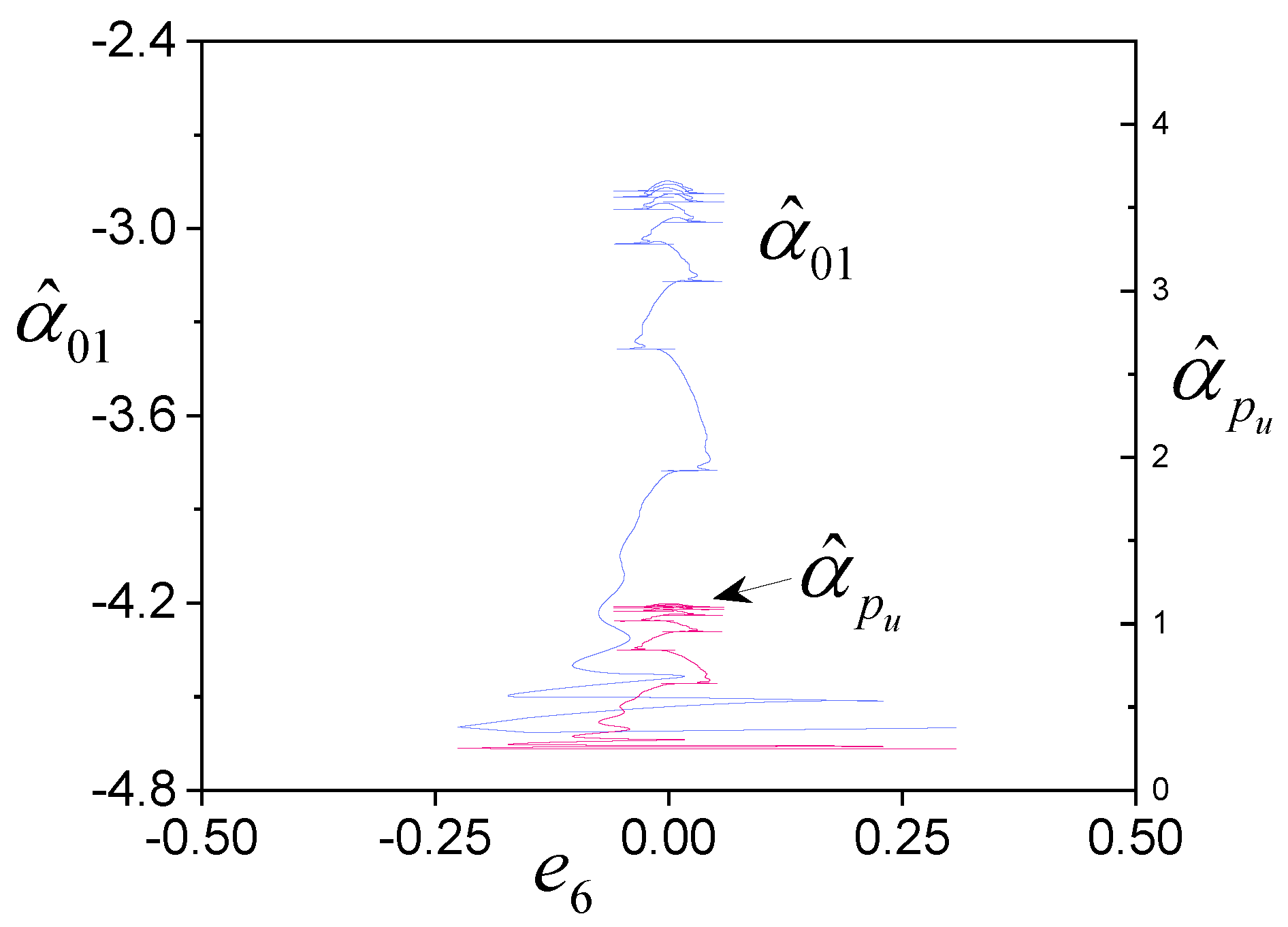
System (38) parameters:

α_{1} = 1.05, β_{1} = 3.5,

α_{2} = 2.2,

β_{2} = 2.2,

μ_{2} = 0.4

α_{01} = 3,

α_{02} = 5.03, β_{0} = 5.2

g (t) = \sin (0.05 π t)

. Simulation results show in Figure 7, Figure 8, Figure 9, Figure 10, Figure 11 and Figure 12.

Figure 7 represents structures (the transition process is excluded) reflecting the phase processes in the system (38). We see that the system is nonlinear. The application of results [31] shows that the system is structurally identifiable. Therefore, the input is S-synchronizing and considers the nonlinear properties of the PLTC.

The analysis shows the relationship between

x_{1}

and

x_{2}

(the correlation coefficient is 0.94). The density diagram (DD) (Figure 8) confirms the influence

x_{1}

and

x_{2}

x_{6}

. We see clear influence boundaries of variables on

x_{6}

. These relationships affect the convergence of adaptive algorithms.

The of adaptive model tuning process for amplitude and phase channels shows in Figure 9, Figure 10.

The tuning of model parameters for the object shows in Figure 11. The tuning process depends on the control action.

The tuning dynamics of model (41) haves a more complex form. The input influence of plays an important role. The theorem 5 statement holds for the PTLCC system.

5. Conclusion

The approach to the identification of interconnected systems proposed. First, the adaptive identification features of TCS with cross-links considered. The conditions of the TCS identifiability in the state space and the output space obtained. Structural aspects of the identification for two-channel systems are considered. WE consider the influence of input properties on the estimation of TCS parameters. Adaptive algorithms are designed for TCS identification with identical channels. Estimates and conditions confirming the estimate convergence of the TCS parameters are obtained. The properties of the adaptive identification system depend on the CL parameters and signal information properties in the TCS.

We consider the interconnected systems. We note the a priori information role in considering existing relationships for identification. It is shown that approaches used for the TCS identification applied to the interconnected system. Adaptive identification examples real systems are considered. We consider TCS with nonlinear control and complex interconnections. The paper considers only certain aspects of this multifaceted subject area. An approach that allows to evaluate the dynamics of processes in the adaptive system is proposed. It considers the influence of system elements on the quality of the parameter tuning process.

Appendix A

Theorem 1 proof.

Consider the Lyapunov function for layer (6)

V_{1} (t) = 0.5 E_{11}^{T} (t) R_{1} E_{11} (t) + 0.5 E_{21}^{T} (t) R_{1} E_{21} (t) .

(A.1)

The derivative of

V_{1} (t)

{\dot{V}}_{1} = E_{11}^{T} Q_{1} E_{11} + E_{11}^{T} R_{1} (Δ A_{1} X_{11} + Δ B_{1} v_{11}) + E_{11}^{T} Q_{1} E_{11} + E_{21}^{T} R_{1} (Δ A_{1} X_{21} + Δ B_{1} v_{21}),

(A.2)

where

R_{1} K_{1} + K_{1}^{T} R_{1} = Q

Q

is symmetric negatively defined matrix.

Since the matrix

K_{1}

is stable, then

E_{11}^{T} Q E_{11} + E_{211}^{T} Q E_{21} \leq - λ_{1} V_{1}

, where

λ_{1} > 0

. Apply the inequality

a b \leq 0.5 (a^{2} + b^{2})

and get

\begin{matrix} {\dot{V}}_{1} \leq - λ_{1} V_{1} + | E_{11}^{T} R_{1} (Δ A_{1} X_{11} + Δ B_{1} v_{11}) | + | E_{21}^{T} R_{1} (Δ A_{1} X_{21} + Δ B_{1} v_{21}) | \leq \\ \leq - λ_{1} V_{1} + 0.5 ({‖ R_{1} E_{11} ‖}^{2} + {‖ R_{1} E_{21} ‖}^{2}) + 0.5 (X_{11}^{T} Δ A_{1}^{T} Δ A_{1} X_{11} + X_{21}^{T} Δ A_{1}^{T} Δ A_{1} X_{21}) + \\ + 0.5 {‖ Δ B_{1} ‖}^{2} (v_{11}^{2} + v_{21}^{2}) . \end{matrix}

(A.3)

g_{i} (t) \in E C_{{\underline{α}}_{i}, {\bar{α}}_{i}} (g_{i})

, and the system (5) is stable and detectable. Therefore, the residuals

Δ A_{1}

Δ В_{1}

K2 are limited. Then (A.3)

\begin{matrix} {\dot{V}}_{1} \leq - (λ_{1} - 0.5) V_{1} + 0.5 (X_{11}^{T} Δ A_{1}^{T} Δ A_{1} X_{11} + X_{21}^{T} Δ A_{1}^{T} Δ A_{1} X_{21}) + \\ + 0.5 {‖ Δ B_{1} ‖}^{2} (v_{12}^{2} + v_{21}^{2}) \leq - (λ_{1} - 0.5) V_{1} + π_{12} {‖ Δ A_{1} ‖}^{2} + 0.5 υ_{12} {‖ Δ B_{1} ‖}^{2}, \end{matrix}

(A.4)

where

π_{12} = 2 \max ({\bar{α}}_{X_{1, 1}}, {\bar{α}}_{X_{2, 1}})

X_{i, 1} (t) \in E C_{{\underline{α}}_{X_{i, 1}}, {\bar{α}}_{X_{i, 1}}}

v_{i 1} (t) \in E C_{{\underline{σ}}_{i 1}, {\bar{σ}}_{i 1}}

υ_{12} = {\bar{σ}}_{11} + {\bar{σ}}_{21}

The system (6) will be stable and identifiable by

Δ A_{1}, Δ B_{1}

π_{12} {‖ Δ A_{1} ‖}^{2} + 0.5 υ_{12} {‖ Δ B_{1} ‖}^{2} \leq (λ_{1} - 0.5) V_{1}

(A.5)

and system variables satisfy conditions 1), 3), 4) of Theorem 1. □

Appendix B

Theorem 2 proof.

Consider the Lyapunov function (10) for layer

k \geq 2

(7). The derivative of

V_{k} (t)

\begin{matrix} {\dot{V}}_{k} = E_{1, k}^{T} Q_{k} E_{1, k} + E_{1, k}^{T} R_{k} (Δ A_{k} X_{1, k} + Δ B_{k} u_{1, k}) + E_{2, k}^{T} Q_{k} E_{2, k} E_{2, k} + \\ + E_{2, k}^{T} R_{k} (Δ A_{k} X_{2, k} + Δ B_{k} u_{2, k}), \end{matrix}

(B.1)

where

Q_{k}

is symmetric negatively defined matrix.

Apply the approach described in Appendix A and get

{\dot{V}}_{k} \leq - (λ_{k} - 0.5) V_{k} + 0.5 {‖ Δ A_{k} ‖}^{2} ({‖ X_{1, k} ‖}^{2} + {‖ X_{2, k} ‖}^{2}) + 0.5 {‖ Δ B_{k} ‖}^{2} (u_{1, k}^{2} + u_{2, k}^{2}) .

(B.2)

Let

{‖ X_{1, k} ‖}^{2} \in E C_{{\underline{α}}_{X_{1, k}}, {\bar{α}}_{X_{1, k}}}, {‖ X_{2, k} ‖}^{2} \in E C_{{\underline{α}}_{X_{2, k}}, {\bar{α}}_{X_{2, k}}}; u_{1, k}^{2} \leq {\bar{α}}_{y_{1, k}} + {| d_{k - 1} (y_{2, k - 1} + d_{k - 2} v_{2, k - 1}) |}^{2},

u_{2, k}^{2} \leq {\bar{α}}_{y_{2, k}} + {| d_{k - 1} (y_{1, k - 1} + d_{k - 2} v_{1, k - 1}) |}^{2}, π_{k, i} = 2 \max ({\bar{α}}_{X_{1, k}}, {\bar{α}}_{X_{2, k}}), y_{2 k - 1} \in E C_{{\underline{α}}_{y_{2, k - 1}}, {\bar{α}}_{y_{2, k - 1}}},

\begin{array}{l} {(d_{k - 1} (y_{1, k - 1} + d_{k - 2} v_{1, k - 1}))}^{2} \leq 2 d_{k - 1}^{2} (y_{1, k - 1}^{2} + {(d_{k - 2} v_{1, k - 1})}^{2}), \\ {(d_{k - 1} (y_{2, k - 1} + d_{k - 2} v_{2, k - 1}))}^{2} \leq 2 d_{k - 1}^{2} (y_{2, k - 1}^{2} + {(d_{k - 2} v_{2, k - 1})}^{2}) . \end{array}

(B.3)

Let

d_{k} (\cdot)

is a constant, i.e.,

d_{k} \leq ω_{k} \leq ω

, where

ω

is some number. Then (B.3)

{(d_{k - 1} (y_{i, k - 1} + d_{k - 2} v_{i, k - 1}))}^{2} \leq 2 ω^{2} ({\bar{α}}_{y_{i, k - 1}} + ω^{2} v_{i, k - 1}^{2}),

(B.4)

Matrices

A_{j}

\forall (j \geq 1)

are stable. Therefore, the

j

-element of each channel is stable and detectable. Applying assumptions made above, we have

v_{i, k - 1}^{2} \in E C_{{\underline{α}}_{v_{i, k - 1}}, {\bar{α}}_{v_{i, k - 1}}}

, and

{(d_{k - 1} (y_{i, k - 1} + d_{k - 2} v_{i, k - 1}))}^{2} \leq 2 ω^{2} ({\bar{α}}_{y_{i, k - 1}} + ω^{2} {\bar{α}}_{v_{i, k - 1}}) .

(B.5)

Then (B.2)

{\dot{V}}_{k} \leq - (λ_{k} - 0.5) V_{k} + 0.5 π_{k, i} {‖ Δ A_{k} ‖}^{2} + 0.5 {‖ Δ B_{k} ‖}^{2} ({\tilde{\bar{α}}}_{k} + 2 ω^{2} β_{k}) .

(B.6)

where

{\tilde{\bar{α}}}_{k} = 2 \max ({\bar{α}}_{y_{2, k - 1}}, {\bar{α}}_{y_{1, k - 1}})

β_{k} = \max_{i} ({\bar{α}}_{y_{i, k - 1}} + ω^{2} {\bar{α}}_{v_{i, k - 1}})

If variables of the system have the property CE and

0.5 π_{k, i} {‖ Δ A_{k} ‖}^{2} + 0.5 {‖ Δ B_{k} ‖}^{2} (\tilde{\bar{α}} + 2 ω^{2} ({\tilde{\bar{α}}}_{k} + 2 ω^{2} β_{k})) \leq (λ_{k} - 0.5) V_{k}

(B.7)

then the system (7) is stable, and, therefore, identifiable by

Δ A_{k}, Δ B_{k}

. □

Appendix C

Theorem 3 proof.

{\dot{V}}_{k} (t)

has the form (B.1), and

v_{i, k - 1}

v_{i, k - 1} = {\begin{cases} {\dot{y}}_{2, k - 1} + {\ddot{v}}_{2, k - 1}, i = 1, \\ {\dot{y}}_{1, k - 1} + {\ddot{v}}_{1, k - 1}, i = 2. \end{cases}

(C.1)

As Theorem 2 condition 4) fulfills system (2) is recoverable. Hence, the derivatives in (C.1) exist and are bounded,

{\dot{y}}_{i, k - 1} (t) \in E C_{{\underline{α}}_{{\dot{y}}_{i, k - 1}}, {\bar{α}}_{{\dot{y}}_{i, k - 1}}}

{\ddot{v}}_{2, k - 1} \in E C_{{\underline{α}}_{{\ddot{v}}_{i, k - 1}}, {\bar{α}}_{{\ddot{v}}_{i, k - 1}}}

. Then

u_{i, k}^{2} \leq {\bar{α}}_{{\dot{y}}_{i, k - 1}} + {\bar{α}}_{{\ddot{v}}_{i, k - 1}}

and (П.2.6)

{\dot{V}}_{k} \leq - (λ_{k} - 0.5) V_{k} + 0.5 π_{k, i} {‖ Δ A_{k} ‖}^{2} + 0.5 {‖ Δ B_{k} ‖}^{2} ({\tilde{\bar{α}}}_{k, \dot{y}} + 2 ({\bar{α}}_{\dot{y}} + {\tilde{\bar{α}}}_{\ddot{v}})),

(C.2)

where

{\tilde{\bar{α}}}_{k, \dot{y}} = \underset{i}{2 \max} {\bar{α}}_{{\dot{y}}_{2 k - 1}}

{\tilde{\bar{α}}}_{k, \ddot{v}} = \underset{i}{2 \max} {\bar{α}}_{{\ddot{v}}_{i, k - 1}}

If variables of the system have the property CE and

0.5 π_{k, i} {‖ Δ A_{k} ‖}^{2} + 0.5 {‖ Δ B_{k} ‖}^{2} ({\tilde{\bar{α}}}_{k, \dot{y}} + 2 ({\bar{α}}_{\dot{y}} + {\tilde{\bar{α}}}_{\ddot{v}})) \leq (λ_{k} - 0.5) V_{k},

then the system (7) is stable, and, therefore, identifiable by

Δ A_{k}, Δ B_{k}

.□

Appendix D

Getting representation (13).

Transfer function for the first equation of the system (1)

y_{1, 1} = C_{1}^{T} {(s I_{q_{1}} - A_{1})}^{- 1} B_{1} v_{11},

(D.1)

where где

I_{q_{1}} \in R^{q_{1} \times q_{1}}

is the unit matrix,

s = d / d t

Let

A_{1}

be the Frobenius matrix with a vector of parameters

A_{1, s} = {[a_{1, s, 1}, a_{1, s, 2}, \dots, a_{1, s, q_{1}}]}^{T}

. Divide the left and right parts (B.1) by the polynomial

v (s) = \prod_{i = 1}^{q_{1} - 1} (s + μ_{i})

, where

μ_{i} > 0

, and obtain the identification representation for

y_{1, 1}

y_{1, 1} (s) = s^{- 1} {b_{1} v_{1, 1} (s) - a_{1, 1} y_{1, 1} (s) + \sum_{i = 2}^{q} (b_{i, i} v_{1, 1} (s) + a_{1, i} y_{1, 1} (s)) \frac{1}{s + μ_{i}}}

(D.2)

\begin{array}{l} {\dot{y}}_{1, 1} = - a_{1, 1} y_{1, 1} + \sum_{m = 2}^{q_{1}} (a_{1, m} p_{y_{1, 1, m}} + b_{1, m} p_{v_{i, 1, m}}) + b_{1, s} v_{1, 1}, \\ {\dot{p}}_{y_{1, 1, m}} = - μ_{i} p_{y_{1, 1, m}} + y_{1, 1}, {\dot{p}}_{v_{i, 1, m}} = - μ_{i} p_{v_{i, 1, m}} + v_{1, 1}, \end{array}

(D.3)

Let

P_{1, 1} ≜ {[y_{1, 1}, p_{y_{1, 1, 1}}, \dots, p_{y_{1, 1, q_{1}}};_{1, 1}, v_{1, 1}, p_{v_{1, 1, 1}}, \dots, p_{v_{1, 1, q_{1}}}]}^{T}

. Then

{\dot{y}}_{1, 1} = {\bar{A}}_{1, 1}^{T} P_{1, 1}, {\bar{A}}_{1, 1}^{T} = [- a_{1, 1}, a_{1, 1, 2}, \dots, a_{1, 1, q_{1}}; b_{1, s}, b_{1, 2}, \dots, b_{1, q_{1}}]

(D.4)

Appendix E

Theorem 4 proof.

Consider the LF

{\tilde{V}}_{1, e} (e_{1, 1}) = 0.5 e_{1, 1}^{2}, {\tilde{V}}_{1, Δ} (Δ {\bar{A}}_{1, 1}) = 0.5 Δ {\bar{A}}_{1, 1}^{T} Γ_{1}^{- 1} Δ {\bar{A}}_{1, 1} .

(E.1)

for the system (16), (21).

Select the element corresponding to

v_{11}

P_{1, 1}

. Let

v_{11} \in E C_{{\underline{α}}_{g_{1}}, {\bar{α}}_{g_{1}}} \ {\bar{E C}}_{{\underline{α}}_{y_{1, n}}, {\bar{α}}_{y_{1}, n}}

, i.e., the variable

v_{11}

is not a constant excitable (the property

E C_{{\underline{α}}_{g_{1}}, {\bar{α}}_{g_{1}}}

dithers by the variable

y_{1, n}

). Therefore,

v_{11} \notin E C_{{\underline{α}}_{v_{11}}, {\bar{α}}_{v_{11}}}

. Then (16) is represented as

{\dot{e}}_{1, 1} = - χ_{1} e_{1, 1} + Δ {\bar{A}}_{1, 1}^{T} P_{1, 1} + f (Δ {\bar{A}}_{1, 1}, p_{v_{11}}),

(E.2)

where

f (\cdot)

is uncertainty caused by CE non-fulfillment of

v_{11}

Remark 9.

v_{11} \in E C_{{\underline{α}}_{g_{1}}, {\bar{α}}_{g_{1}}} \ {\bar{E C}}_{{\underline{α}}_{y_{1, n}}, {\bar{α}}_{y_{1} . n}}

is not a set operation. This is the operation on properties.

Then

\begin{matrix} {\dot{\tilde{V}}}_{1, e} = - χ_{1} e_{1, 1}^{2} + e_{1, 1} (Δ {\bar{A}}_{1, 1}^{T} P_{1, 1} + f) \leq - χ_{1} e_{1, 1}^{2} + | e_{1, 1} Δ {\bar{A}}_{1, 1}^{T} P_{1, 1} | + | e_{1, 1} f | \leq \\ \leq - \frac{χ_{1}}{2} e_{1, 1}^{2} + \frac{1}{χ_{1}} Δ {\bar{A}}_{1, 1}^{T} P_{1, 1} P_{1, 1}^{T} Δ {\bar{A}}_{1, 1} + \frac{1}{χ_{1}} f^{2} \leq - \frac{χ_{1}}{2} e_{1, 1}^{2} + \frac{1}{χ_{1}} π_{P_{1, 1}} {‖ Δ {\bar{A}}_{1, 1} ‖}^{2} + \frac{1}{χ_{1}} f^{2}, \end{matrix}

(E.3)

where

‖ P_{1, 1} P_{1, 1}^{T} ‖ \leq {\bar{π}}_{P_{1, 1}} < {\bar{α}}_{P_{1, 1}}

f

it is limited as

f

contains a component that is uncompensated by the adaptive algorithm. Therefore

{| f |}^{2} \leq α_{f}

, where

α_{f} \geq 0

and

α_{f} \neq {\bar{α}}_{v_{1, 1}}

. So

{\dot{\tilde{V}}}_{1, e} \leq - \frac{χ_{1}}{2} {\tilde{V}}_{1, e} + \frac{2}{χ_{1}} π_{P_{1, 1}} {\tilde{V}}_{1, Δ} + \frac{α_{f}}{χ_{1}} .

(E.4)

Consider

{\dot{\tilde{V}}}_{1, Δ} = - e_{1, 1} Δ {\bar{A}}_{1, 1}^{T} P_{1, 1}

. Let

\exists υ \leq 1

exist for

t > > t_{0}

, which is true

e_{1, 1} Δ {\bar{A}}_{1, 1}^{T} P_{1, 1} = υ (e_{1, 1}^{2} + Δ {\bar{A}}_{1, 1}^{T} P_{1, 1} P_{1, 1}^{T} Δ {\bar{A}}_{1, 1})

and

λ_{\max}^{- 1} (Γ_{1}) {‖ Δ {\bar{A}}_{1, 1} ‖}^{2} \leq {\tilde{V}}_{1, Δ} \leq λ_{\min}^{- 1} (Γ_{1}) {‖ Δ {\bar{A}}_{1, 1} ‖}^{2}

, где

λ_{\min} (Γ_{1}), λ_{\max} (Γ_{1})

are the minimum and maximum eigenvalues of the matrix

Γ_{1}

. Then

Δ {\bar{A}}_{1, 1}^{T} P_{1, 1} P_{1, 1}^{T} Δ {\bar{A}}_{1, 1} \geq {\underline{π}}_{P_{1, 1}} {‖ Δ {\bar{A}}_{1, 1} ‖}^{2} \geq {\underline{π}}_{P_{1, 1}} λ_{\min} (Γ_{1}) {\tilde{V}}_{1, Δ}

(E.5)

And

{\dot{\tilde{V}}}_{1, Δ} = - e_{1, 1} Δ {\bar{A}}_{1, 1}^{T} Γ_{1} P_{1, 1} \leq - 2 υ {\tilde{V}}_{1, e} - 2 υ η {\tilde{V}}_{1, Δ}

(E.6)

where

{\underline{π}}_{P_{1, 1}} \geq 0

η = {\underline{π}}_{P_{1, 1}} λ_{\min} (Γ_{1})

Transform the right side (E.6)

\begin{array}{l} - 2 υ {\tilde{V}}_{1, e} - 2 υ η {\tilde{V}}_{1, Δ} = - υ (η {\tilde{V}}_{1, Δ} \pm 2 \sqrt{2 η {\tilde{V}}_{1, Δ} {\tilde{V}}_{1, e}} + 2 {\tilde{V}}_{1, e}) - υ η {\tilde{V}}_{1, Δ} = \\ = - υ {(\sqrt{{\tilde{V}}_{1, e}} + \sqrt{2 η {\tilde{V}}_{1, Δ}})}^{2} + 2 υ \sqrt{2 η {\tilde{V}}_{1, Δ} {\tilde{V}}_{1, e}} - υ η {\tilde{V}}_{1, Δ} \leq \\ \leq - υ η {\tilde{V}}_{1, Δ} + 2 υ \sqrt{2 η {\tilde{V}}_{1, Δ} {\tilde{V}}_{1, e}} . \end{array}

- 2 υ η {\tilde{V}}_{1, Δ} - 2 υ {\tilde{V}}_{1, e} \leq - υ η {\tilde{V}}_{1, Δ} + 2 υ \sqrt{2 η {\tilde{V}}_{1, Δ} {\tilde{V}}_{1, e}}

, then (E.6)

{\dot{\tilde{V}}}_{1, Δ} \leq - υ η {\tilde{V}}_{1, Δ} + 2 υ \sqrt{2 η {\tilde{V}}_{1, Δ} {\tilde{V}}_{1, e}}

(E.7)

Apply the inequality

- a z^{2} + b z \leq - \frac{- a z^{2}}{2} + \frac{b^{2}}{2 a}, a > 0, b \geq 0, z \geq 0

and obtain

{\dot{\tilde{V}}}_{1, Δ} \leq - υ η {\tilde{V}}_{1, Δ} + 2 υ \sqrt{2 η {\tilde{V}}_{1, Δ} {\tilde{V}}_{1, e}} \leq - \frac{υ η}{2} {\tilde{V}}_{1, Δ} + 4 υ {\tilde{V}}_{1, e}

(E.8)

Functions

{\dot{\tilde{V}}}_{1, e} \in M^{+}

{\dot{\tilde{V}}}_{1, Δ} \in M^{+}

and we have a system of inequalities for the system (16), (21)

[\begin{matrix} {\dot{\tilde{V}}}_{1, e} \\ {\dot{\tilde{V}}}_{1, Δ} \end{matrix}] \leq \underset{A_{S_{1}}}{\underset{︸}{[\begin{matrix} - \frac{χ_{1}}{2} & 2 \frac{π_{P_{1, 1}}}{χ_{1}} \\ 4 υ & - \frac{υ η}{2} \end{matrix}]}} \underset{{\tilde{V}}_{1, e, Δ}}{\underset{︸}{[\begin{matrix} {\tilde{V}}_{1, e} \\ {\tilde{V}}_{1, Δ} \end{matrix}]}} + \underset{B_{S_{1}}}{\underset{︸}{[\begin{matrix} \frac{α_{f}}{χ_{1}} \\ 0 \end{matrix}]}} .

(E.9)

Comparison system (CS) for (E.9):

{\dot{S}}_{1} (t) = A_{S_{1}} S_{1} (t)

, where

S_{1} (t) = {[s_{1, e} (t), s_{1, Δ} (t)]}^{T}

s_{1, w} (t)

(w = e, Δ)

is a majorant for

V_{1, w} (t)

, and

s_{1, w} (t_{0}) \geq V_{1, w} (t_{0}) .

CS is stable if [30]

{(- 1)}^{i} Δ_{i} (A_{S_{1}}) > 0

, where

Δ_{i} (A_{S_{1}})

is main

i

-minor of the matrix

A_{S_{1}} .

The condition stability has the form

χ_{1}^{2} η > 32 π_{P_{1, 1}}

. We get the estimate from (E.9)

{\tilde{V}}_{1, e, Δ} (t) \leq e^{A_{S_{1}} (t - t_{0})} S_{1} (t_{0}) + \int_{t_{0}}^{t} e^{A_{S_{1}} (t - τ)} B_{S_{1}} d τ

(E.10)

Exponential dissipation of the system (14)–(16), (22) follows from (E.10).ν

Appendix F

Theorem 5 proof.

As from Theorem 4 follows, the input of the system (19), (20), (25)

P_{1, k} \notin E C_{{\underline{α}}_{P_{1, k}}, {\bar{α}}_{P_{1, k}}}

P_{1, k} \notin E C_{{\underline{α}}_{P_{1, k}}, {\bar{α}}_{P_{1, k}}}

follows from

P_{1, k} = P_{1, k} (u_{1, k}) \Rightarrow {u_{1, k} = υ_{u_{1, k}} (y_{1, k - 1}, v_{1, k - 1})} \Rightarrow P_{1, k} (y_{1, k - 1}, v_{1, k - 1})

Arguments of

u_{1, k}

do not have a CE property. Write the equation (20) as

{\dot{e}}_{1, k} = - χ_{k} e_{1, k} + Δ {\bar{A}}_{1, k}^{T} P_{1, k} + f_{1, k} ({\bar{A}}_{1, k} P_{1, k})

(F.1)

where

f_{1, k} (\cdot) \in ℝ

is the uncertainty that is the result from

P_{1, 1} \notin E C_{{\underline{α}}_{P_{1, 1}}, {\bar{α}}_{P_{1, 1}}}

. Since

{\bar{A}}_{1, k}, P_{1, k}

are limited, then

f_{1, k}^{2} \leq α_{f_{1, k}}

, where

α_{f_{1, k}} \geq 0

Apply (F.1) and get for

{\dot{\tilde{V}}}_{k, e}

\begin{matrix} {\dot{\tilde{V}}}_{k, e} = - χ_{k} e_{1, k}^{2} + e_{1, k} (Δ {\bar{A}}_{1, k}^{T} P_{1, k} + f_{1, k}) \leq - \frac{χ_{k}}{2} e_{1, k}^{2} + \frac{1}{2 χ_{k}} {(Δ {\bar{A}}_{1, k}^{T} P_{1, k} + f_{1, k})}^{2} \leq \\ \leq - \frac{χ_{k}}{2} e_{1, k}^{2} + \frac{2}{2 χ_{k}} Δ {\bar{A}}_{1, k}^{T} P_{1, k} P_{1, k}^{T} Δ {\bar{A}}_{1, k} + \frac{2}{2 χ_{k}} f_{1, k}^{2} \leq \\ \leq - χ_{k} {\tilde{V}}_{k, e} + \frac{2 ϑ_{P_{1, k}}}{χ_{k}} {\tilde{V}}_{k, Δ} + \frac{α_{f_{1, k}}}{χ_{k}}, \end{matrix}

(F.2)

where

‖ P_{1, k} P_{1, k}^{T} ‖ \leq π_{P_{1, k}} < {\bar{α}}_{P_{1, k}}

λ_{\max}^{- 1} (Γ_{k}) {‖ Δ {\bar{A}}_{1, k} ‖}^{2} \leq {\tilde{V}}_{k, Δ} \leq λ_{\min}^{- 1} (Γ_{k}) {‖ Δ {\bar{A}}_{1, k} ‖}^{2}

ϑ_{P_{1, k}} = π_{P_{1, k}} λ_{\max} (Γ_{k})

So,

{\dot{\tilde{V}}}_{k, e} \leq - χ_{k} {\tilde{V}}_{k, e} + \frac{2 ϑ_{P_{1, k}}}{χ_{k}} {\tilde{V}}_{k, Δ} + \frac{α_{f_{1, k}}}{χ_{k}}

Consider

{\dot{\tilde{V}}}_{k, Δ}

. We apply (21) and obtain

{\dot{\tilde{V}}}_{k, Δ} = - e_{1, k} Δ {\bar{A}}_{1, k}^{T} P_{1, k}

. Let

\exists υ \leq 1

exist for

t > > t_{0}

, which is true

e_{1, k} Δ {\bar{A}}_{1, k}^{T} P_{1, k} = υ (e_{1, k}^{2} + Δ {\bar{A}}_{1, k}^{T} P_{1, k} P_{1, k}^{T} Δ {\bar{A}}_{1, k})

Then

Δ {\bar{A}}_{1, k}^{T} P_{1, k} P_{1, k}^{T} Δ {\bar{A}}_{1, k} \geq {\underline{π}}_{P_{1, k}} {‖ Δ {\bar{A}}_{1, k} ‖}^{2} \geq {\underline{π}}_{P_{1, k}} λ_{\min} (Γ_{k}) {\tilde{V}}_{k, Δ}

(F.3)

and

{\dot{\tilde{V}}}_{k, Δ} = - e_{1, k} Δ {\bar{A}}_{1, k}^{T} Γ_{k} P_{1, k} \leq - 2 υ {\tilde{V}}_{k, e} - 2 υ η {\tilde{V}}_{k, Δ},

(F.4)

where

{\underline{π}}_{P_{1, k}} \geq 0

η = {\underline{π}}_{P_{1, k}} λ_{\min} (Γ_{k})

. Transform the right side (F.4)

\begin{array}{l} - 2 υ {\tilde{V}}_{k, e} - 2 υ η {\tilde{V}}_{k, Δ} = - υ (η {\tilde{V}}_{k, Δ} \pm 2 \sqrt{2 η {\tilde{V}}_{k, Δ} {\tilde{V}}_{k, e}} + 2 {\tilde{V}}_{k, e}) - υ η {\tilde{V}}_{k, Δ} = \\ \leq - υ η {\tilde{V}}_{k, Δ} + 2 υ \sqrt{2 η {\tilde{V}}_{k, Δ} {\tilde{V}}_{k, e}} . \end{array}

So,

{\dot{\tilde{V}}}_{k, Δ} \leq - υ η {\tilde{V}}_{k, Δ} + 2 υ \sqrt{2 η {\tilde{V}}_{k, Δ} {\tilde{V}}_{k, e}}

(F.5)

\begin{matrix} {\dot{\tilde{V}}}_{k, Δ} \leq - υ η {\tilde{V}}_{k, Δ} + 2 υ \sqrt{2 η {\tilde{V}}_{k, Δ} {\tilde{V}}_{k, e}} \leq - \frac{υ η}{2} {\tilde{V}}_{k, Δ} + \frac{8 η υ^{2}}{2 υ η} {\tilde{V}}_{k, e} = \\ = - \frac{υ η}{2} {\tilde{V}}_{k, Δ} + 4 υ {\tilde{V}}_{k, e} . \end{matrix}

(F.6)

{\dot{\tilde{V}}}_{1, e} \in M^{+}

{\dot{\tilde{V}}}_{1, Δ} \in M^{+}

, then we get the system of inequalities

[\begin{matrix} {\dot{\tilde{V}}}_{k, e} \\ {\dot{\tilde{V}}}_{k, Δ} \end{matrix}] \leq \underset{A_{S_{k}}}{\underset{︸}{[\begin{matrix} - \frac{χ_{k}}{2} & 2 \frac{ϑ_{P_{1, k}}}{χ_{k}} \\ 4 υ & - \frac{υ η}{2} \end{matrix}]}} \underset{{\tilde{V}}_{k}}{\underset{︸}{[\begin{matrix} {\tilde{V}}_{k, e} \\ {\tilde{V}}_{k, Δ} \end{matrix}]}} + \underset{B_{S_{k}}}{\underset{︸}{[\begin{matrix} \frac{α_{f_{1, k}}}{χ_{k}} \\ 0 \end{matrix}]}} .

(F.7)

χ_{k}^{2} η_{k} > 32 ϑ_{P_{1, k}}

, then the CS

{\dot{S}}_{k} (t) = A_{S_{k}} S_{k} (t) + B_{S_{k}}

is stable for (F.7). We get an upper-bound estimate for the quality of the adaptive system (19), (20), (25) from (F.7)

{\tilde{V}}_{k} (t) \leq e^{A_{S_{k}} (t - t_{0})} S_{k} (t_{0}) + \int_{t_{0}}^{t} e^{A_{S_{k}} (t - τ)} B_{S_{k}} d τ . ■

(F.8)

References

Morozovsky, V.E. Multi-connected automatic control systems. Moscow: Energiya, 1970.
Zyryanov, G.V. Control systems for multi-connected objects: a textbook. Chelyabinsk: SUSU Publishing Center, 2010.
Meerov M.V., Litvak B.L. Optimization of multicommunicated control systems. Moscow: Nauka, 1972.
Bukov V.N., Maksimenko I.M., Ryabchenko V.N. Control of multivariable systems. Autom. Remote Control; 1998; 6; 97–110.
Voronov, A.A. Introduction in dynamics of complex controlled systems. Moscow: Nauka, 1985.
Egorov I.N., Umnov V.P. Control systems for electric drives of technological robots and manipulators: textbook. Vladimir: Publishing house of Vladimir State University, 2022.
Egorov, I.N. Positional force control of robotic and mechatronic devices. Vladimir: Publishing House of Vladimir State University, 2010.
Gupta N., Chopra N. Stability analysis of a two-channel feedback networked control system. Conference: 2016 Indian Control Conference (ICC), 2016;8.
Pawlak А., Hasiewicz Z. Non-parametric identification of multi-channel systems by multiscale expansions. 2002 IEEE International Conference on Acoustics, Speech, and Signal Processing, 2011.
Kholmatov U. The possibility of applying the theory of adaptive identification to automate multi-connected objects. The American journal of engineering and technology, 2023, 31-38.
Aliyeva A.S. Identification of multiconnected dynamic objects with uncertainty based on neural technology and reference converters. Informatics and Control Problems, 2019;39(2);93-102.
Hua C., Guan X., Shi P. Decentralized robust model reference adaptive control for interconnected time-delay systems. Proceeding of the 2004 American Control Conference Boston, Massachusetts June 30 - July 2, 2004;4285-4289. [CrossRef]
Gupta N., Chopra N. Stability analysis of a two-channel feedback networked control system. Conference: 2016 Indian Control Conference (ICC), 2016.
Glentis G.-O. and Slump C. H. A highly modular normalized adaptive lattice algorithm for multichannel least squares filtering. International Conference on Acoustics, Speech, and Signal Processing, 1995.
Ali M., Abbas H., Chughtai S. S. and Werner H. Identification of spatially interconnected systems using neural network. 49th IEEE Conference on decision and control (CDC), 2011.
Yang Q., Zhu M., Jiang T. He J., Yuan J., and Han J. Decentralized robust adaptive output feedback stabilization for interconnected nonlinear systems with uncertainties, Journal of control science and engineering, 2016;2016;3656578;12. [CrossRef]
Wu H. Decentralized adaptive robust control of uncertain large-scale non-linear dynamical systems with time-varying delays. IET Control Theory and Applications, 2012;6(5);629–640. [CrossRef]
Fan H., Han L., Wen C., and Xu L. Decentralized adaptive output-feedback controller design for stochastic nonlinear interconnected systems. Automatica, 2012;48;11. [CrossRef]
Ali M., Chughtai S.S, Werner H. Identification of spatially interconnected systems. Proceedings of the 48h IEEE Conference on Decision and Control (CDC) held jointly with 2009 28th Chinese Control Conference, 2010.
Ioannou P. A. Decentralized adaptive control of interconnected systems. IEEE Transactions on automatic control, 1986;ac-31(4);291-298. [CrossRef]
Sanandaji B.M., Vincent T.L., Wakin M.B. A review of sufficient conditions for structure identification in interconnected systems. IFAC proceedings volumes, 2012;45(16);1623-1628. [CrossRef]
Soverini U., Söderström T. Blind identification of two-channel FIR systems: a frequency domain approach, IFAC PapersOnLine 53-2, 2020;914–920. [CrossRef]
Huang Y., Benesty J., Chen J. Adaptive blind multichannel identification. In: Benesty, J., Sondhi, M.M., Huang, Y.A. (eds) Springer Handbook of Speech Processing. Springer Handbooks. Springer, Berlin, Heidelberg. 2008.
Benesty J., Paleologu C., Dogariu L.-M., and Ciochină S. Identification of linear and bilinear systems: a unified study. Electronics, 2021;10(1790);33. [CrossRef]
Bretthauer G., Gamaleja T., Wilfert H.-H. Identification of parametric and nonparametric models for MIMO closed loop systems by the correlation method. IFAC Proceedings Volumes, 1984;17(2);753-758. [CrossRef]
Lomov A.A. On quantitative a priori measures of identifiability of coefficients of linear dynamic systems. Journal of computer and systems sciences international, 2011;50;1–13.
Krasovsky A. A. On two-channel automatic control systems with antisymmetric connections. Automation and telemechanics. 1957,18(2),126–136.
Karabutov N.N. On adaptive identification of systems having multiple nonlinearities. Russ. Technol. J. 2023;11(5);94−105. [CrossRef]
Karabutov N.N. Adaptive identification of systems. Moscow: URSS, 2007.
Gantmacher F. R. The theory of matrices. AMS Chelsea Publishing, 2000.
Karabutov N. Structural identifiability of systems with multiple nonlinearities. Contemporary Mathematics, 2021;2(2); 140-161. [CrossRef]
Barsky A.G. On the theory of two-dimensional and three-dimensional automatic control systems. Moscow: Logos, 2015.
Skorospeshkin M.V. Adaptive two-channel correction device for automatic control systems. Bulletin of the Tomsk Polytechnic University, 2008;312(5):52-57.

Figure 1. Evaluation of structure for cross-links.

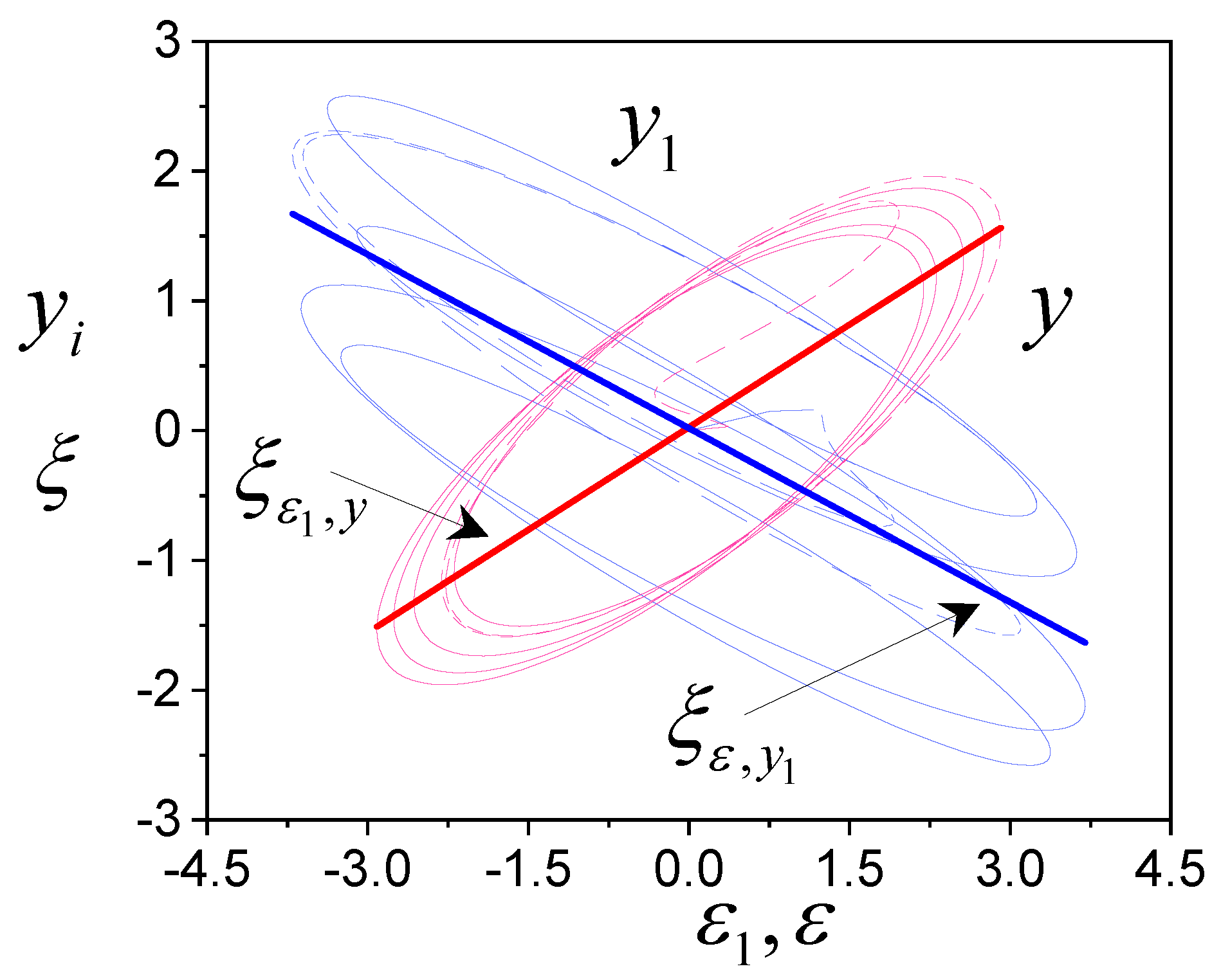
Figure 2. Tuning model (36.1) parameters.

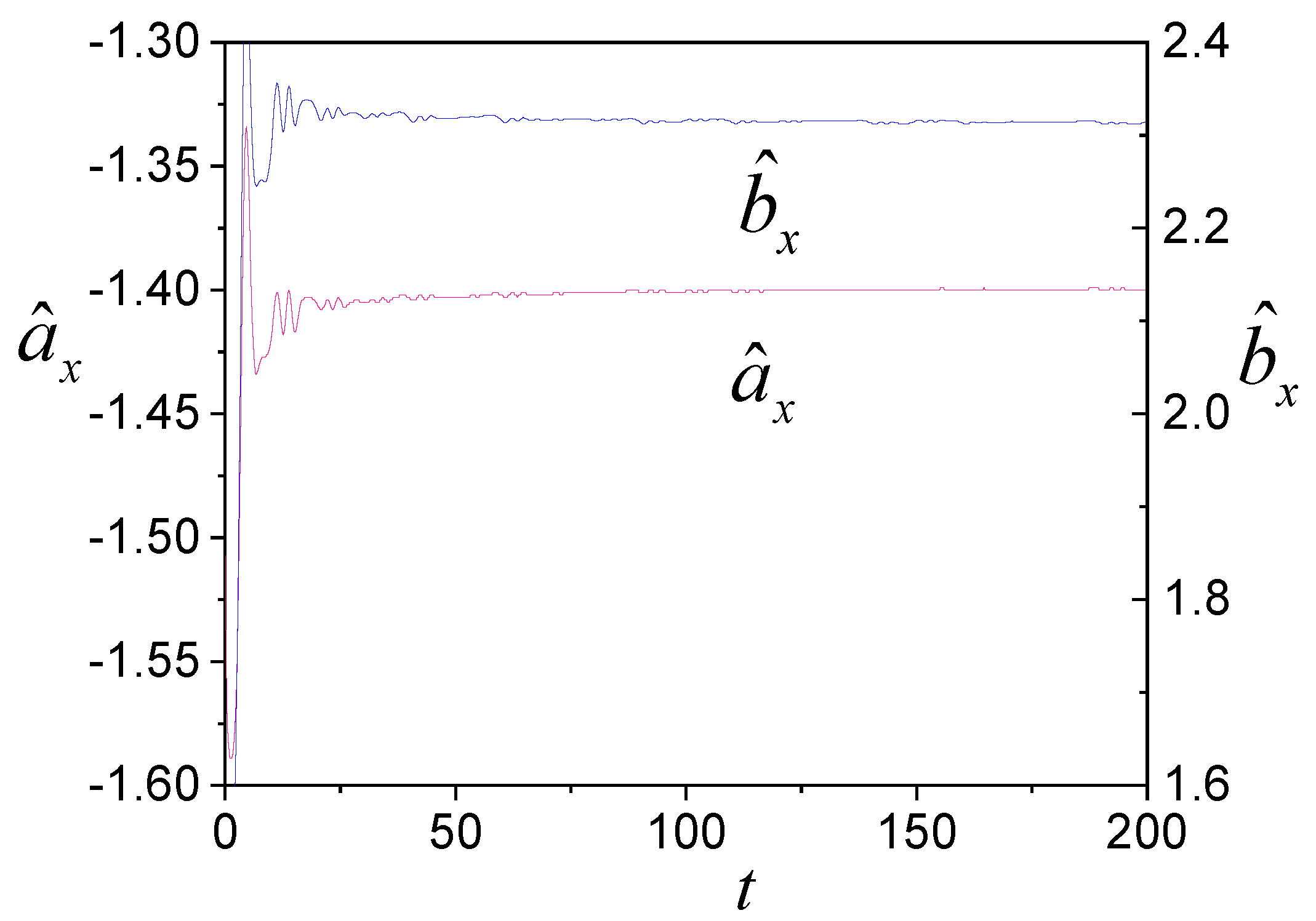
Figure 3. Tuning model (36.2) parameters.

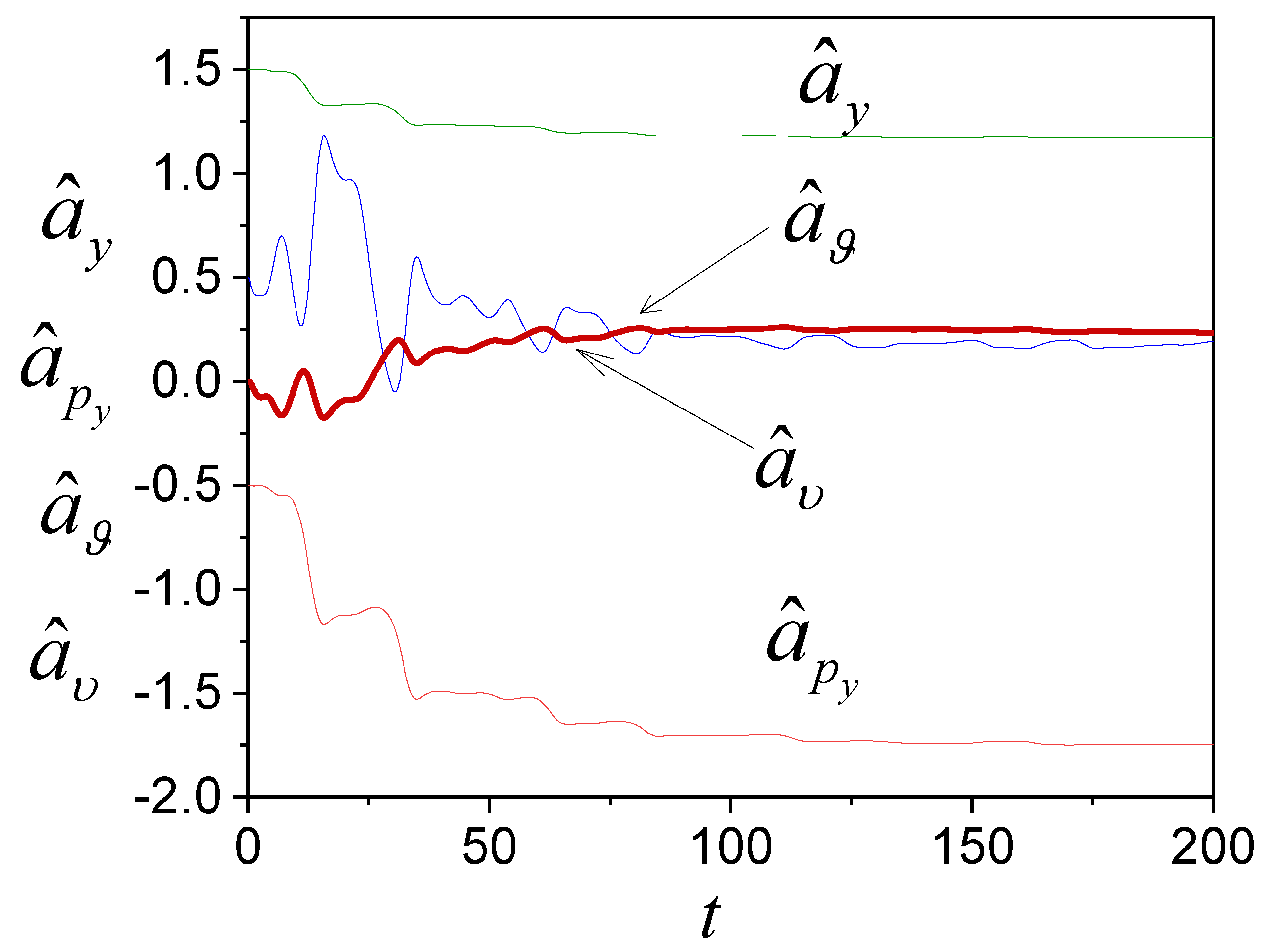
Figure 4. Changing identification error.

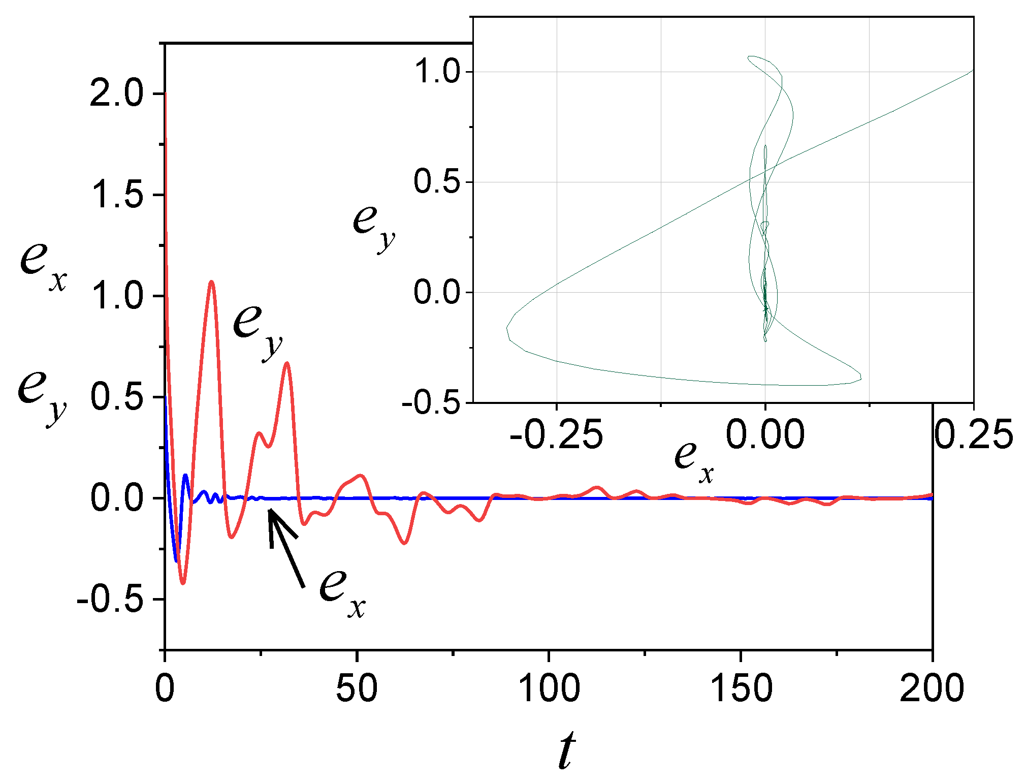
Figure 5. Tuning model (36.2) parameters.

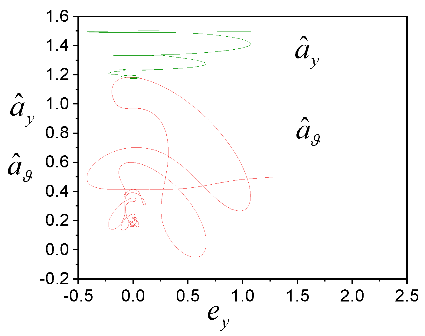
Figure 6. Tuning model (36.2) parameters.

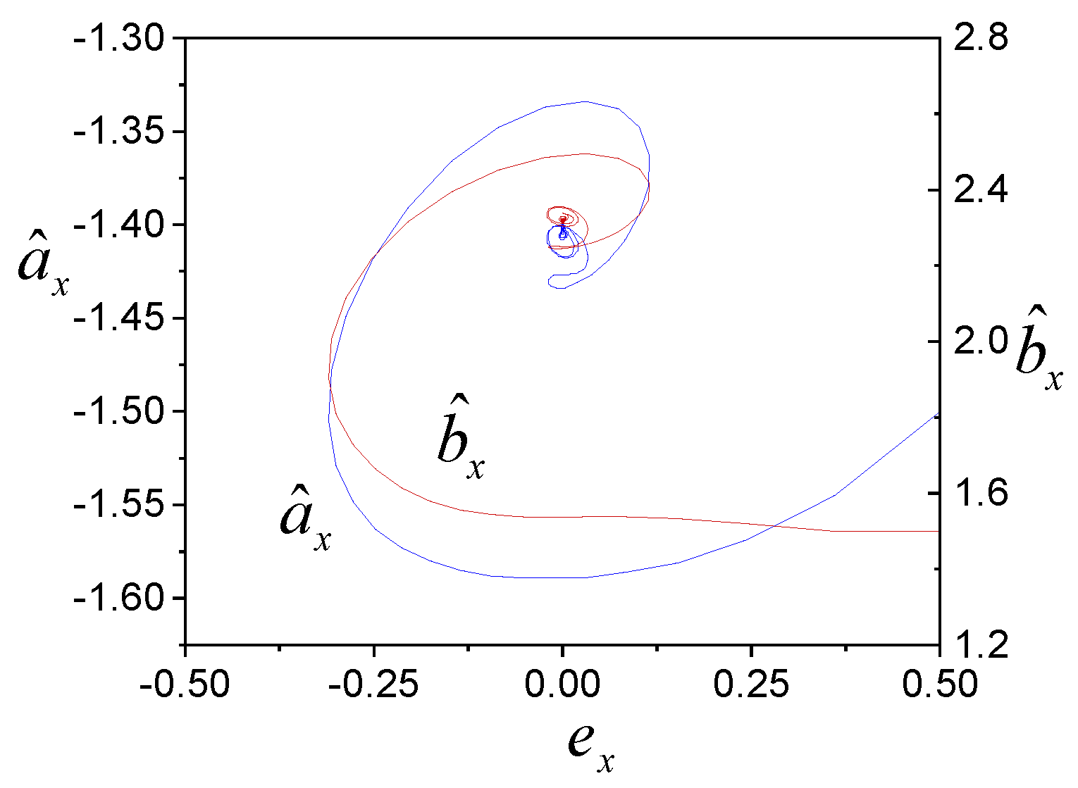
Figure 7. Phase portraits of system (38) (1 −

x_{6} (x_{2})

, 2−

x_{6} (x_{1})

Figure 7. Phase portraits of system (38) (1 −

x_{6} (x_{2})

, 2−

x_{6} (x_{1})

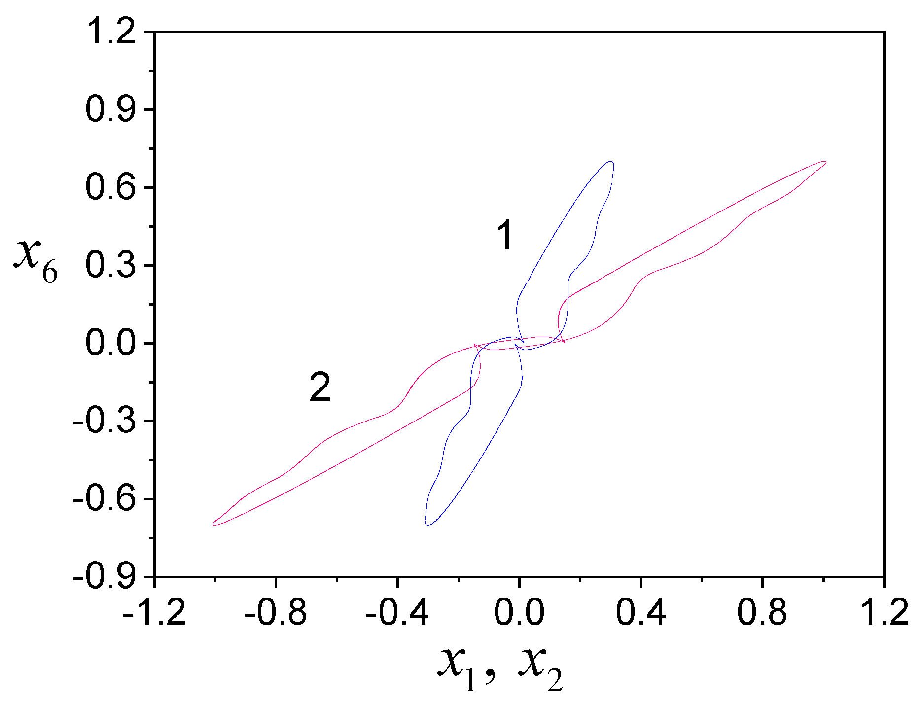
Figure 8. Effect evaluation of variables

x_{1}, x_{2}

x_{6}

Figure 8. Effect evaluation of variables

x_{1}, x_{2}

x_{6}

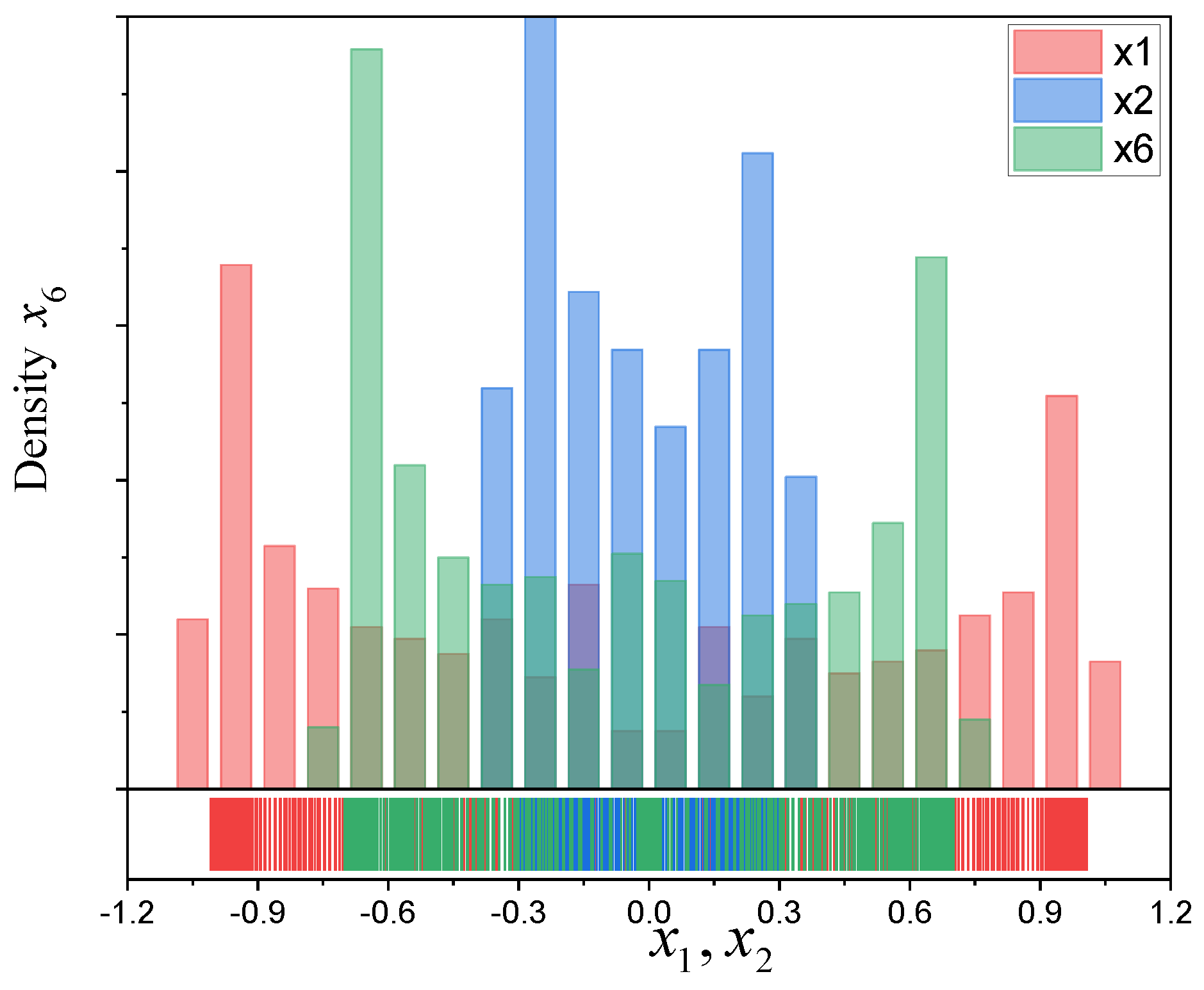
Figure 9. Tuning model parameters (39).

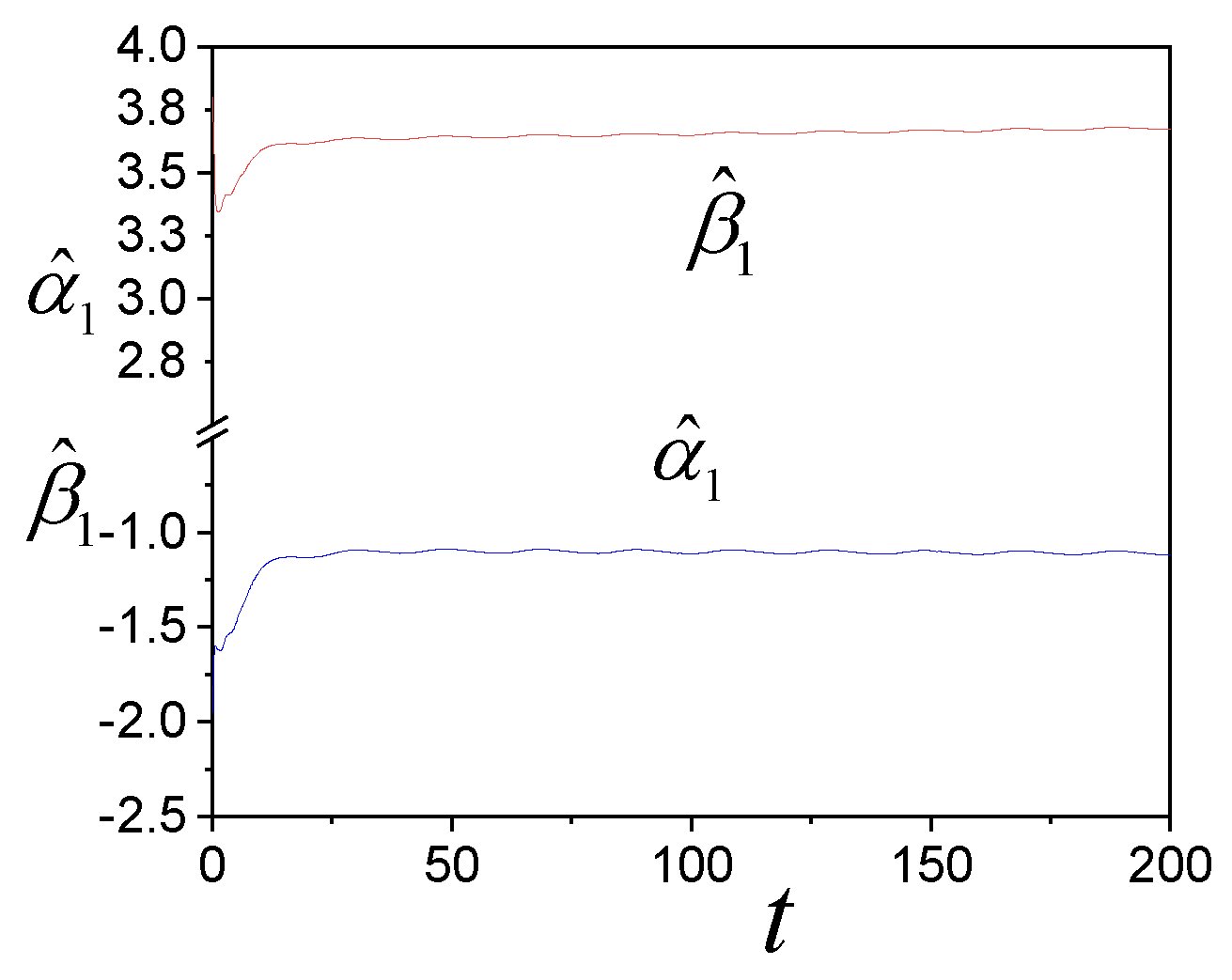
Figure 10. Tuning model parameters (40).

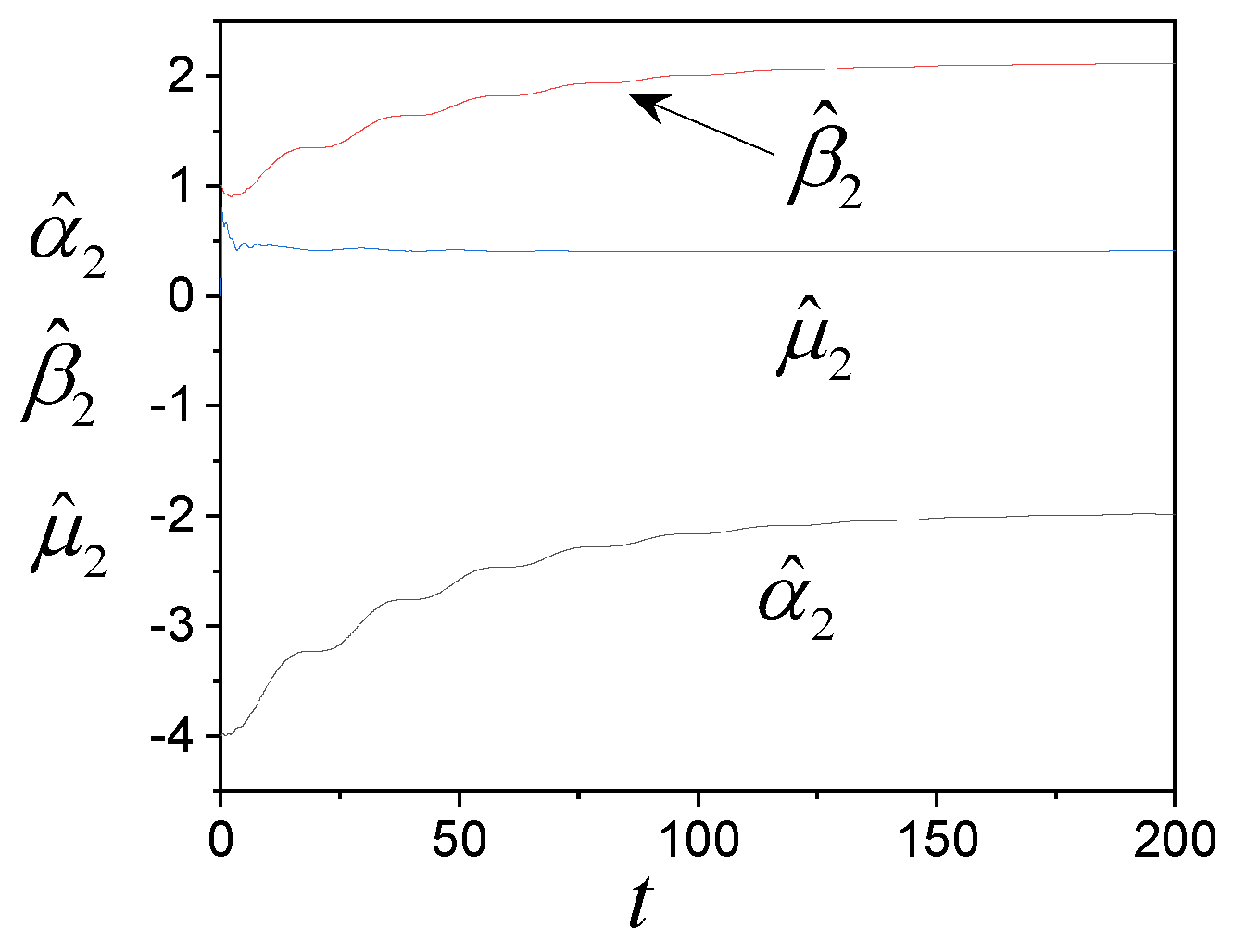
Figure 11. Tuning model parameters (41).

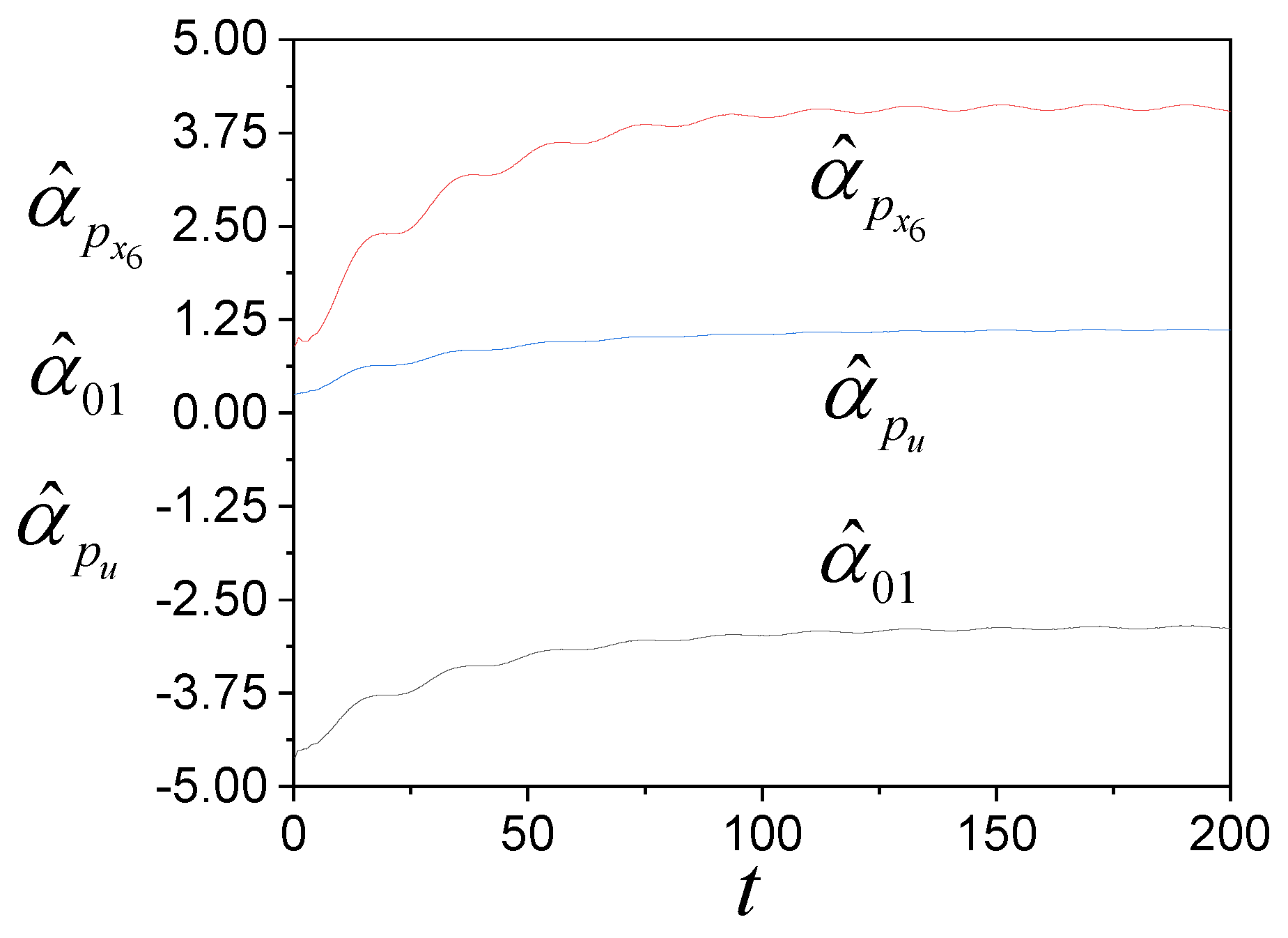
Figure 12. The dynamics of contour for tuning model (40).

Disclaimer/Publisher’s Note: The statements, opinions and data contained in all publications are solely those of the individual author(s) and contributor(s) and not of MDPI and/or the editor(s). MDPI and/or the editor(s) disclaim responsibility for any injury to people or property resulting from any ideas, methods, instructions or products referred to in the content.

© 2024 by the authors. Licensee MDPI, Basel, Switzerland. This article is an open access article distributed under the terms and conditions of the Creative Commons Attribution (CC BY) license (http://creativecommons.org/licenses/by/4.0/).

Copyright: This open access article is published under a Creative Commons CC BY 4.0 license, which permit the free download, distribution, and reuse, provided that the author and preprint are cited in any reuse.

MDPI Initiatives

Important Links

Choose an area of interest and we will send you notifications of new preprints at your preferred frequency.

Disclaimer

On Adaptive Identification of Interconnected Systems

Abstract

1. Introduction

2. Two-channel systems

2.1. Problem Setting

2.2. About TCS structural aspects

2.3. TCS Adaptive identification

3. Interconnected systems

4. Examples

5. Conclusion

Appendix A

Theorem 1 proof.

Appendix B

Theorem 2 proof.

Appendix C

Theorem 3 proof.

Appendix D

Getting representation (13).

Appendix E

Theorem 4 proof.

Appendix F

Theorem 5 proof.

References

MDPI Initiatives

Important Links

Subscribe