Disaggregation Model: A Novel Methodology to Estimate Customers Profiles in a Low-Voltage Distribution Grid Equipped With Smart Meters

In a context of increasingly necessary energy transition, precise modelling of profiles for low-voltage (LV) network consumers is crucial to enhance hosting capacity. Typically, load curves for these consumers are estimated through measurement campaigns conducted by Distribution System Operators (DSO) for a representative subset of customers or through the aggregation of load curves from household appliances within a residence. With the instrumentation of smart meters becoming more common, a new approach to modelling profiles for residential customers is proposed to make the most of the measurements from these meters. The disaggregation model estimates the load profile of customers on a low-voltage network by disaggregating the load curve measured at the secondary substation level. By utilizing only the maximum power measured by Linky smart meters, along with the load curve of the secondary substation, this model can estimate the daily profile of customers. For 48 secondary substations in our dataset, the model obtained an average symmetric mean average percentage error (SMAPE) error of 4.91% in reconstructing the load curve of the secondary substation from the curves disaggregated by the model. This methodology can allow the estimation of the daily consumption behaviors of the low-voltage customers. In this way, we can safely envision solutions that enhance the grid hosting capacity.

Keywords:

Subject: Engineering - Electrical and Electronic Engineering

1. Introduction

The international negotiations on climate policies reveal that we are grappling with the impacts we have on the environment. One way to mitigate these impacts directly involves reducing the use of fossil fuels and increasing electrification. This leads to changes in the level the distribution electrical network is used. These changes extend from the generation and distribution of energy to the way customers use it. They are part of a phenomenon called energy transition. Its effects can be immediately seen when we look at the new directive of the European Union, "Fit for 55," which aims to reduce greenhouse gas emissions by 55% by 2030. To achieve this goal, one of the proposals is to increase the renewable energy target from 32% to at least 40% by 2030 [1].

We can also take a closer look at the energy transition by examining the French scenario in more detail. According to data from the DSO Enedis, responsible for energy distribution in 95% of metropolitan France, the number of production sites connected to the grid increased by 178% between the years 2012 and 2023. The same data show us that the total number of electric vehicle charging infrastructures connected to the grid grew by 2000% between 2015 and 2023 [2]. The French Ministry of Ecological Transition estimates the distribution of residential energy use in France by type. The heating system represents approximately 70% of the country's residential energy consumption. Among the various energy sources used for residential heating, electric sources have been growing proportionally year after year, as indicated by this data [3]. We can therefore observe that the fight against environmental impacts is reflected in a significant change in the habits of electricity production and consumption, centered in the distribution grid.

As the uses of the grid evolve, the distribution grid also evolves to keep pace with these changes. The electrical grids are becoming more digital, transforming our networks into smart grids. According to the International Energy Agency, “smart grids are electrical networks that use digital technologies, sensors, and software to better match the supply and demand for electricity in real-time while minimizing costs and maintaining the stability and reliability of the network.” The major enabler of this digitization lies in the replacement of electricity meters, transitioning from analog/digital meters to smart meters. Smart meters are electronic devices that record information such as electrical energy consumption and communicate this information to the consumer, electricity providers, and DSOs.

We can look at some examples of this evolution in the metering landscape around the world. The Italian DSO ENEL initiated the deployment of its first generation of smart meters in 2001 for your 32 million customers [4]. In 2016, the Italian regulatory body defined the minimum functions for the new generation of meters. This new generation of meters began to be distributed in 2017, with the aim of making energy consumption more sustainable and becoming a key element in the construction of smarter and more circular cities [5]. The U.S. DSO PG&E launched the SmartMeter™ program for the installation of smart meters in 2006, and the majority of its customers were equipped with them by 2012 [6]. The Canadian DSO BC Hydro is the primary electricity distributor in the British Columbia region, serving over 4 million customers in most areas of the province. The deployment of smart meters began in 2011 and was completed in 2012 [7]. The Korean Electric Power Corporation, KEPCO, is one of the largest energy companies in South Korea. Since 2012, the KEPCO has installed approximately 120,000 smart meters to promote the smart grid infrastructure. Until 2018, 6.8 million households in South Korea were equipped with smart meters. The goal was to reach 22.5 million households by the early 2020s [8]. TEPCO, the largest Japanese DSO, completed the installation of approximately 29 million smart meters by the end of 2020 [9]. The French DSO Enedis began rolling out its meters in 2015 and, from 2023 last figures, has over 37 million smart meters deployed. [10] It is possible to observe that the change in the metering landscape is a global phenomenon, occurring in parallel with changes in grids usage.

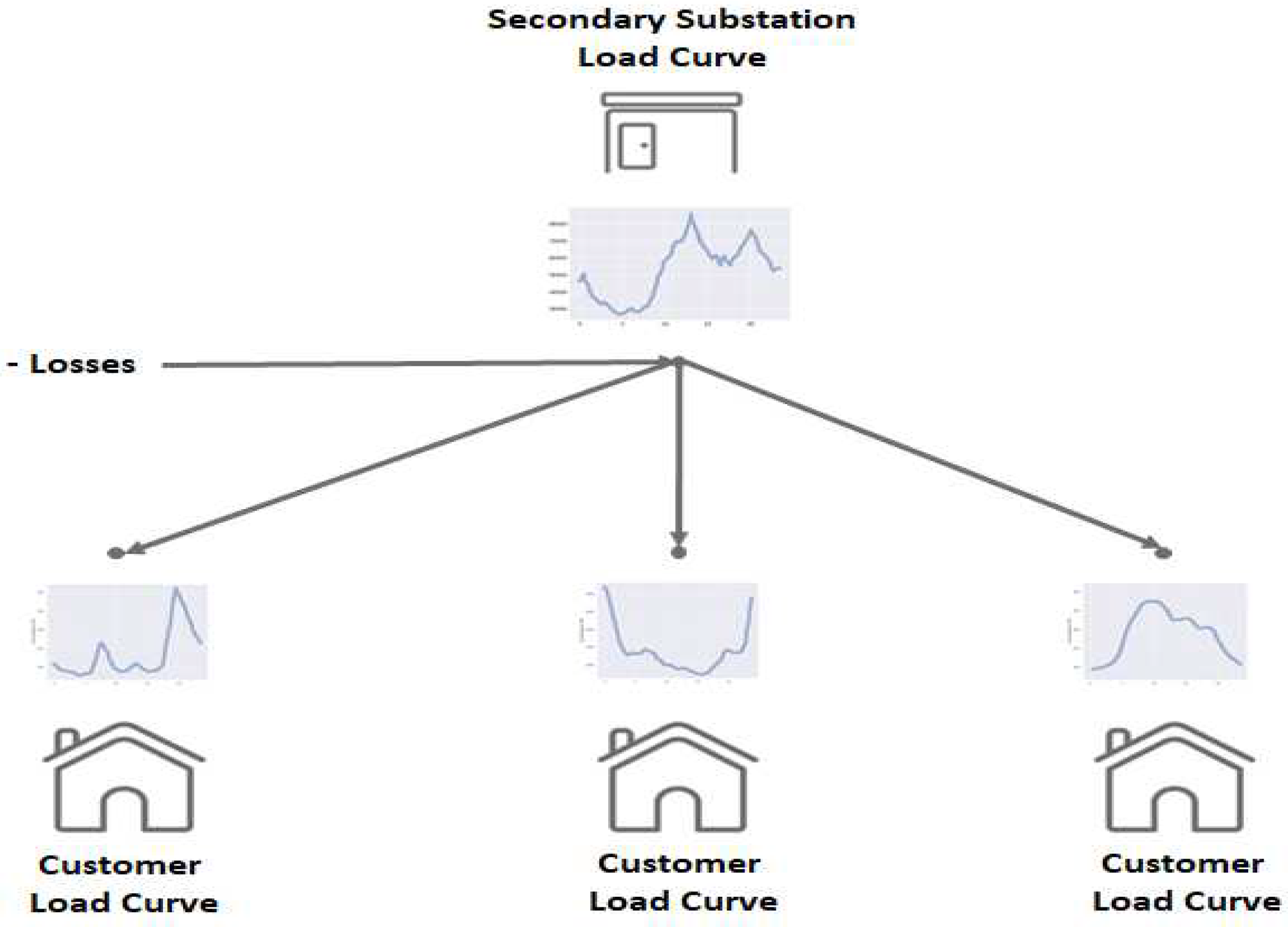
The exploitation of smart meter data makes it possible to explore new solutions that helps the grid to receive this new usage in the energy transition context. The objective of this paper is to propose a novel methodology to estimate the load curves of consumers on the low-voltage network using very few data from smart meters. This modelling will be based on data provided by the French DSO Enedis, but the model had been built to be compliant with data from most smart metering infrastructure. The possible constraints that may be faced when using smart meter data for load curve estimation are related to data privacy concerns and IT infrastructure limitations. The aim of this model is to explore the use of smart meter data for profile or load curve estimation and be a model that can be employed to assist in the integration of new usages. To achieve this, the model starts with the load curve of the secondary substation and disaggregates it into individual load curves of customers, as illustrated in Figure 1. The idea behind this model is to perform daily disaggregation, allowing us to access the customer-level load curve every day. The customer load curve is the input data for network calculation tools, enabling us to compute voltage and power transits in the network. With this daily customer-generated load curve data, it is possible to better estimate the hosting capacity of the network as well as the available flexibility of the demand.

Looking at the literature, T. Barbier [11] conducted a classification of different types of electrical consumption models. This classification is based on two factors. The first factor is a framework with three levels of consumption, including the individual level of the customer and their devices, the aggregated level by type of customer and type of device, as well as the aggregated level of the customer by spatial zone and their devices. The second factor is a framework of variables influencing consumption, including the device inventory, the technology of these devices, usage behavior, socioeconomic level, meteorology, variables related to the place of consumption, customer subscription, and the electricity market. Thus, he lands at 6 categories of models.

The first category includes models based on aggregated consumptions in a zone. This category includes models where the scale is the level of electrical consumption aggregated by spatial zone. These models primarily focus on the temporal component of consumption and are commonly referred to as “forecasting” models. In this category, [12,13,14,15] stand out in the analysis and evaluation of this type of forecasting model.

The second category consists of models based on consumptions by type of customer. This category includes models where the scale is the level of consumption per type of customer. This type of modelling produces different load curves for each type of customer (residential, industrial, etc.), and customers of the same type will have identical profiles, adjusted in energy [16,17,18]. This category can be subdivided based on the model's input data.

According to the author [11], the third category consists of models based on consumption by usage. An example of this type of model is one that decomposes thermosensitive uses from non-thermosensitive uses based on load curves from different zones [19]. It illustrates the example of thermosensitivity in France, allowing the Transmission System Operator and Distribution System Operators to understand the influence of meteorological hazards on network sizing.

The next category consists of models based on consumption by type of customer and usage. This category essentially includes models for the residential sector that are based on consumption by type of use of equipment in the sector. This category comprises models [20,21,22] that involve disaggregating electrical consumption profiles with information on the ownership rate of devices and possibly with socio-economic data. These are “bottom-up” and “top-down” models.

The fifth category consists of models based on consumption per customer. According to the author [1], models belonging to this category use data from smart meters to make short-term predictions of electrical consumption for individual customers [23,24,25].

The last category consists of models based on consumption per device. This category aims to estimate consumption at different levels through the aggregation of device consumption. An example of this is Non-Intrusive Load Monitoring models [26,27,28]. The idea is to have a sufficiently fine temporal resolution of measurements to capture the energy signatures of different devices.

Based on this analysis of the classification of different types of electricity consumption models conducted in [11], we can conclude that "bottom-up" and "top-down" models are the ones that come closest to the initial idea of disaggregation models. However, the scale at which we intend to build the disaggregation model is that of the secondary substation level to assess the load curve or profile of each LV customer attached to it. This is not clearly represented in this classification. The load curves of customers are the inputs for the DSO's tools to carry out network planning studies. Therefore, estimating them accurately becomes a necessary task in this context of evolving network usage. The use of usage decomposition methodologies such as "bottom-up" proves to be extremely dependent on measurements with fine temporal resolution. DSOs may not necessarily have this degree of precision in their measurements. Our disaggregation model avoids this situation, making it more accessible.

This literature review confirms that we are seeking to undertake innovative research that will contribute to expanding the horizons of the field. Keeping this in mind, let us explore the idea novel methodology into details.

2. Materials and Methods

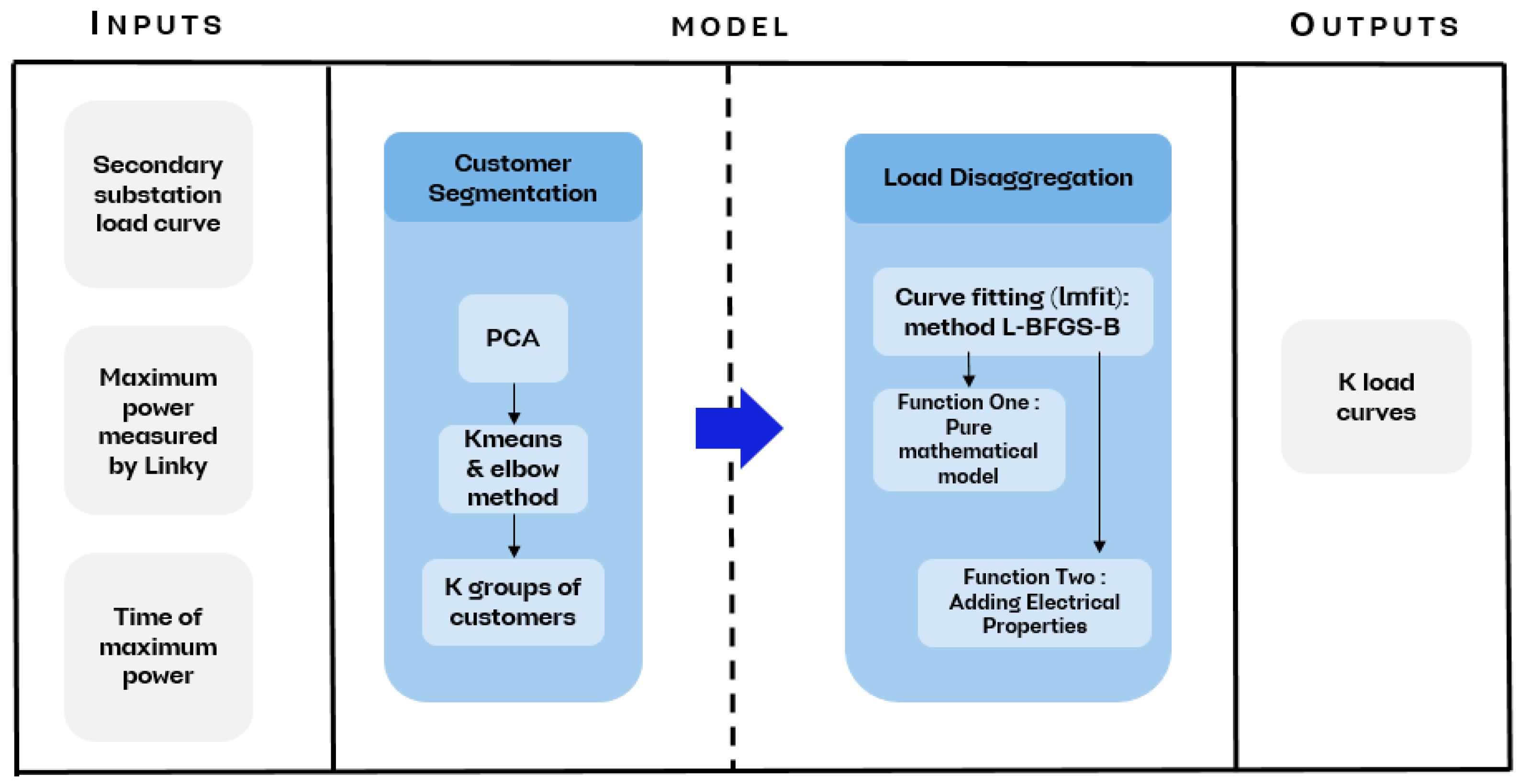
The general principle of the model is to disaggregate the load curve of the substation into load curves for each downstream customer. To achieve this, we will carry out this process in two steps:

Customer Segmentation: The N customers of a substation share similar characteristics, either because they belong to the same categories (residential, professional, etc.) or because they have similar consumption habits. In this perspective, the segmentation (or the number of clusters) of these customers is performed to identify K groups of similar customers among the N customers of the substation, where K < N.
Secondary Substation Load Disaggregation: The load curve of the substation is then disaggregated into K curves, representing the K groups of similar customers at the substation. These K curves are then adjusted in energy to assign to each customer the curve of the group to which they belong.

The data scope chosen for the development of this model included 48 secondary substations, where load curve data was collected for the period from March 2022 to March 2023. Additionally, maximum power and energy data from Linky smart meters (a total of 5318 meters) were collected downstream of these substations for each day of the period. It is essential to specify that the Linky data of the customers used in this study are associated with a customer panel, who have given their consent to Enedis for the use of their data in the context of network studies. Including the one integrated into this article, in accordance with the General Data Protection Regulation (GDPR). Therefore, these data are not accessible beyond this perimeter. We have three types of information per secondary substation:

The load curve of the substation.
The maximum power value in watts measured by Linky for all customers connected in the substation.
The time of day (hours and minutes) when the maximum power occurred.

With all this information in mind, we can delve into the details of each step of the model.

2.1. Customer Segmentation

The objective of this step is to identify K groups of similar customers at a substation with N customers. The idea behind this is to simplify the subsequent disaggregation step, as we will disaggregate the substation's load curve into fewer curves (K < N). Additionally, working at an individual customer level is extremely complex due to the significant variability in consumption. Therefore, working at a slightly higher level (K groups of similar customers) is considered the optimal strategy. Various temporal scales could be used to segment customers at a substation, such as daily, by days of the week, monthly, seasonal, yearly, among others.

A segmentation by season was chosen as it offers more advantages. It provides a sufficient volume of data for customer segmentation and allows to visualize the evolution of the behavior of all customers over time. Customers who exhibit similar behavior within a given season may not necessarily show similar behavior in other seasons. The data selected for building this dataset are maximum power data. The decision to use only this data is to simplify the construction process by leveraging one of the pieces of information collected by Linky meters. Moreover, the simpler the information used in model construction, the easier it will be to reproduce it in other research.

To preprocess the data, the dimensionality reduction technique called Principal Component Analysis (PCA) was employed [29]. PCA is a statistical technique used to reduce the dimensionality of data while preserving, as much as possible, the essential information contained in the data. Specifically, this method is beneficial for reducing the size of processed data, limiting data redundancy, and facilitating easier data visualization, leading to better understanding [29].

In the literature, various methods exist for performing segmentation. For the implementation of this disaggregation model step, we chose to work with partition methods, specifically k-means [30], due to their simplicity in understanding the proposed results. Kmeans clustering is one of the most well-known and widely used unsupervised learning algorithms. Generally, unsupervised algorithms make inferences from datasets using only input vectors without reference to known or labeled outcomes [31]. The goal of Kmeans clustering is to group similar data points and discover underlying clusters. To determine the number of groups K that will be assigned in our dataset, the elbow method [32] is employed. It aims to identify the number of clusters K that strikes a good balance between reducing the sum of squared errors (SSE) and the complexity of the model. It is an easy-to-understand and apply method, making it a practical tool for choosing K. However, the drawback is the subjectivity of the method, as identifying the elbow can be challenging. For this reason, we chose to use the Python library Kneed [33] to automatically detect elbows and eliminate the subjective aspect. The Figure 2 illustrates the step of customer segmentation.

2.2. Secondary Substation Load Disaggregation

The objective of this step is to formulate a method to disaggregate the load curve of a secondary substation into K curves that represent the K groups among the N customers identified in the segmentation step. To begin thinking about how to achieve this solution, let start by formulating the problem mathematically.

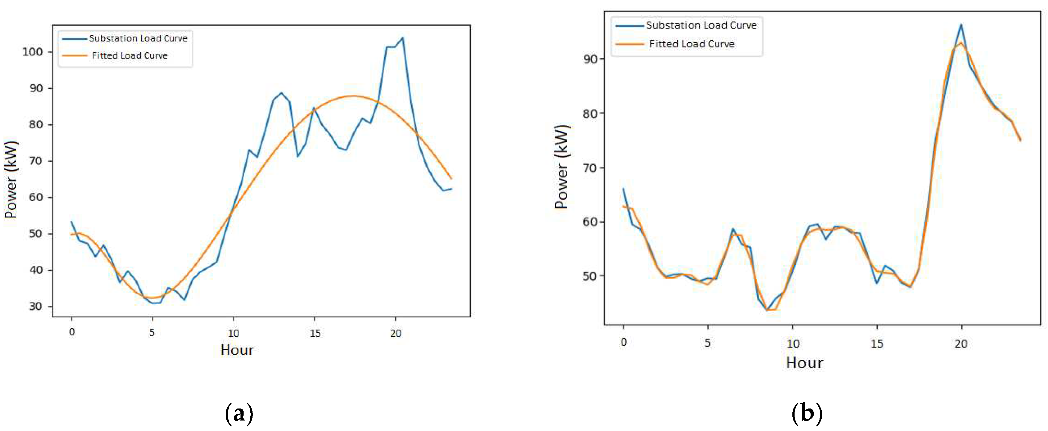
{L o a d C u r v e}_{\begin{matrix} s e c o n d a r y \\ s u b s t a t i o n \end{matrix}} = \sum_{k = 1}^{K} C l u s t e r C u r v e (k)

(1)

As shown in Equation 1, the disaggregation of the substation's load curve can be seen as the sum of K curves being equal to the substation's curve. Approaching the problem from this perspective, once the equations describing the K curves are defined, this problem can be solved by applying a curve fitting method. Curve fitting is a commonly used technique in data analysis to estimate the parameters of a mathematical function that best describes a set of data [34]. Its basic principle is to find the optimal parameters of a mathematical function that minimizes the square of the difference between the observed data and the values predicted by the function, as shown in Equation 2:

m i n (\sum_{i = 1}^{M} {(y_{i} - f (x_{i}, θ))}^{2})

(2)

The goal is to find 𝜃_{𝑜𝑝𝑡𝑖𝑚𝑎𝑙} values that minimize quadratic error, called the cost function. In other words, curve fitting involves solving an optimization problem where the objective is to identify the values of the parameters 𝜃 that make the cost function as small as possible. To solve this curve fitting problem, the Python library lmfit [35] was chosen. As explained by the developers, lmfit provides a user-friendly interface for defining models, specifying parameters, fitting data, and retrieving results. It also allows the choice of a variety of optimization methods. In the case of this disaggregation problem, the chosen method is L-BFGS-B (Limited-memory Broyden-Fletcher-Goldfarb-Shanno with Bound constraints) [36]. With the definition of how the disaggregation problem will be approached, it is now necessary to define which mathematical function best describes our data. The data on which the curve fitting will be performed are the daily load curves of the secondary substations.

2.2.1. Function One – Pure Mathematical Model

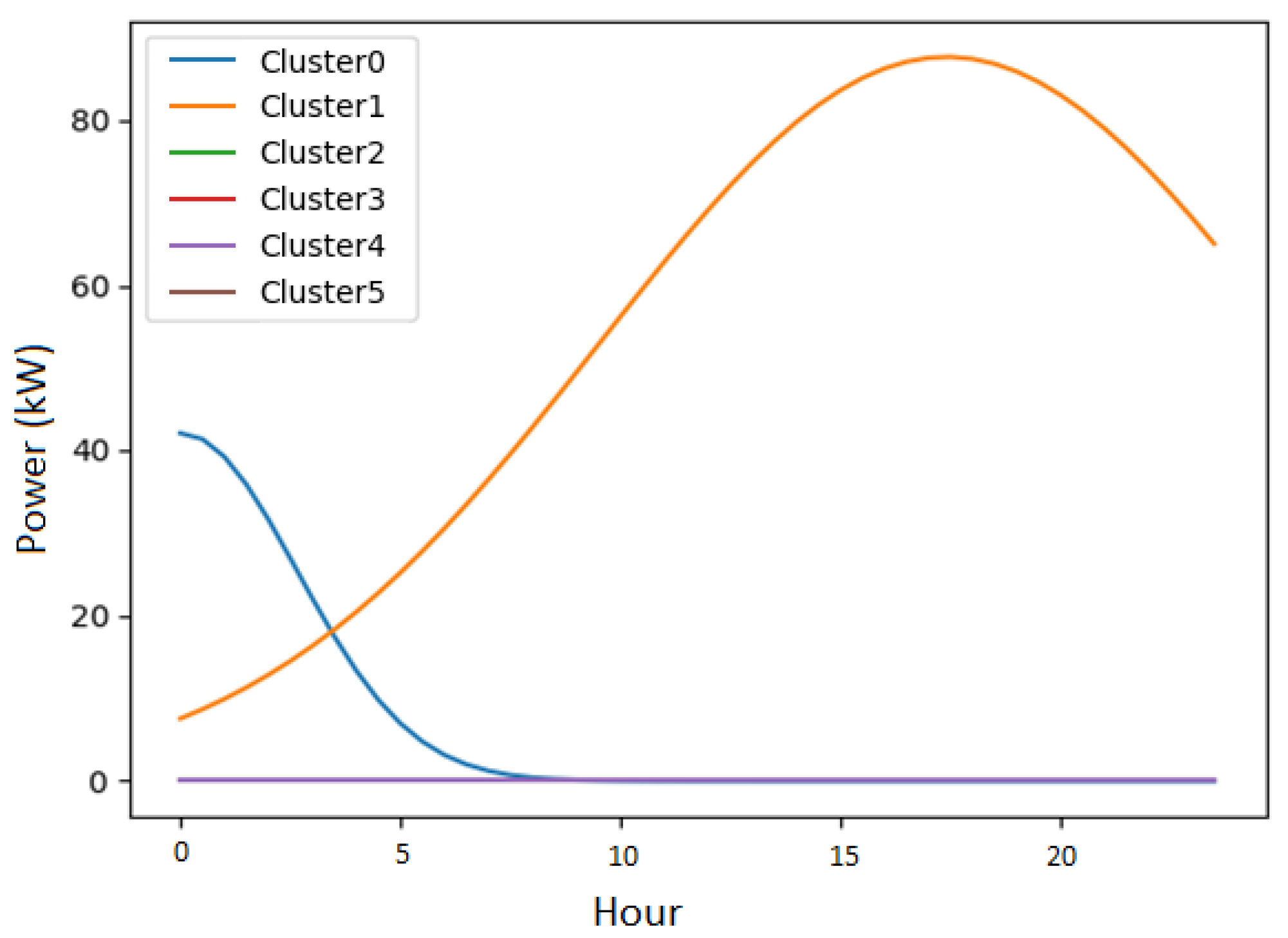
The option chosen to address the question of which equations best describe the sum of K curves in Equation 2 is a sum of N Gaussians, as shown in Equation 3.

f (x, a, b, c) = \sum_{k = 1}^{N} (a_{k} * {e x p}^{\frac{{- (x - b_{k})}^{2}}{{2 * c}_{k}^{2}}})

(3)

Where: formally θ in the function f(x, θ) now corresponds to the parameters

a_{k}

b_{k}

c_{k}

a_{k}

determines the height of the Gaussian,

b_{k}

determines the position of the center of the Gaussian, and

c_{k}

determines the width of the Gaussian.

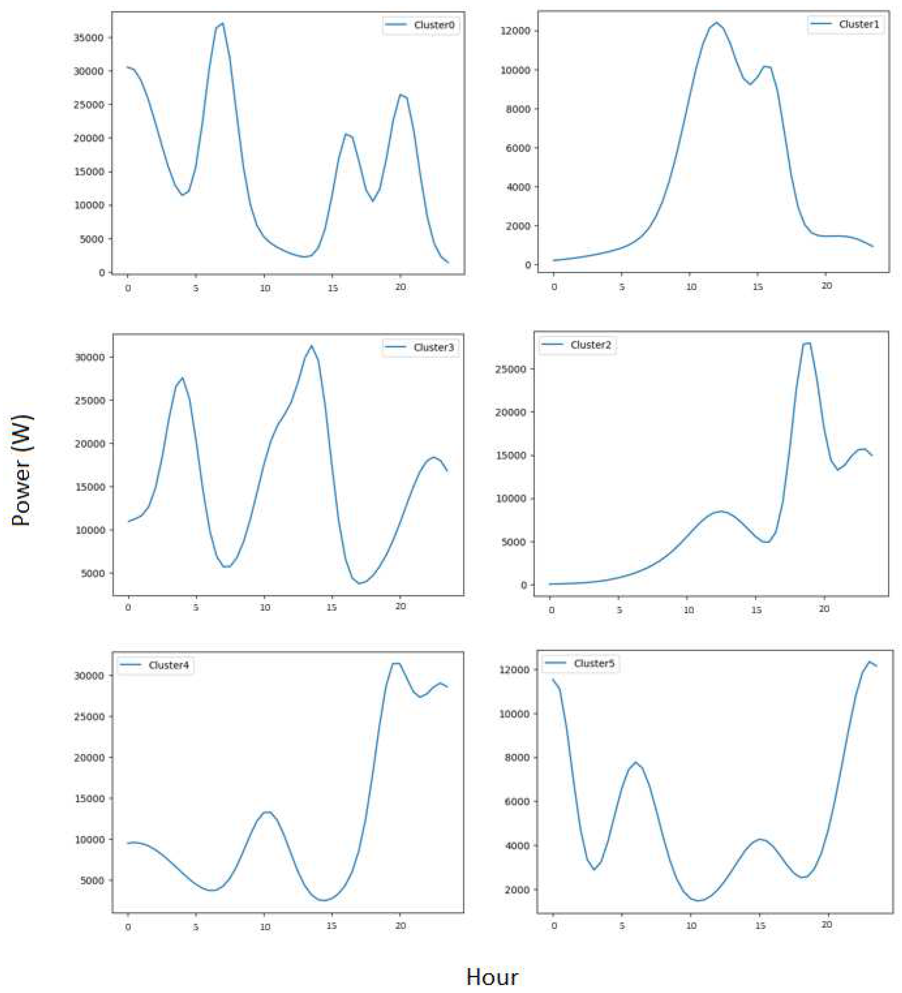
The reason that leads to believe that this assumption is a good starting point is as follows: if we examine the shape of customer load profiles [37,38], the consumption peaks at different times of the day resemble Gaussian behavior. These profiles represent the behavior of a group of customers belonging to the same class. Furthermore, a Gaussian is a natural candidate because it is a classic function in statistics related to the central limit theorem. This theorem plays a fundamental role in statistical theory by showing that the mean of many independent and identically distributed random variables approximately follows a Gaussian distribution, regardless of the initial distribution of these variables. This demonstrates its ubiquity in modeling random phenomena, such as the electrical consumption of low-voltage customers.

2.2.2. Function Two – Adding Electrical Properties to the Purely Mathematical Model

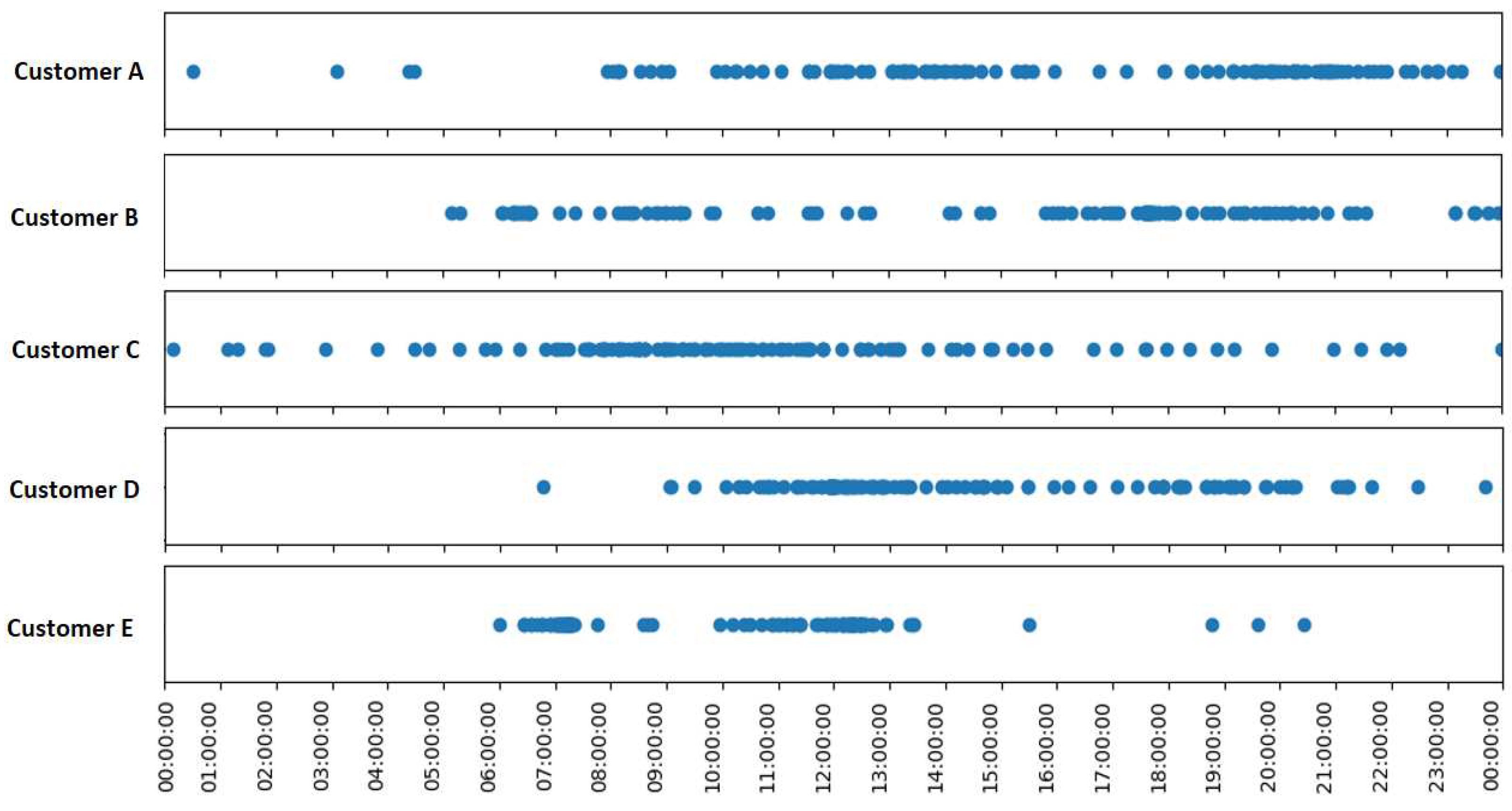
The idea behind this function is to use the information available thanks to Linky meters to approximate the modeling of the real behavior of network customers. Starting with an analysis for a single customer, all the times at which their maximum power was recorded during the season can be examined. It can be observed that these times are not always identical. This is illustrated in Figure 3, where each blue point represents an occurrence of maximum power for 5 examples of customers during the winter season.

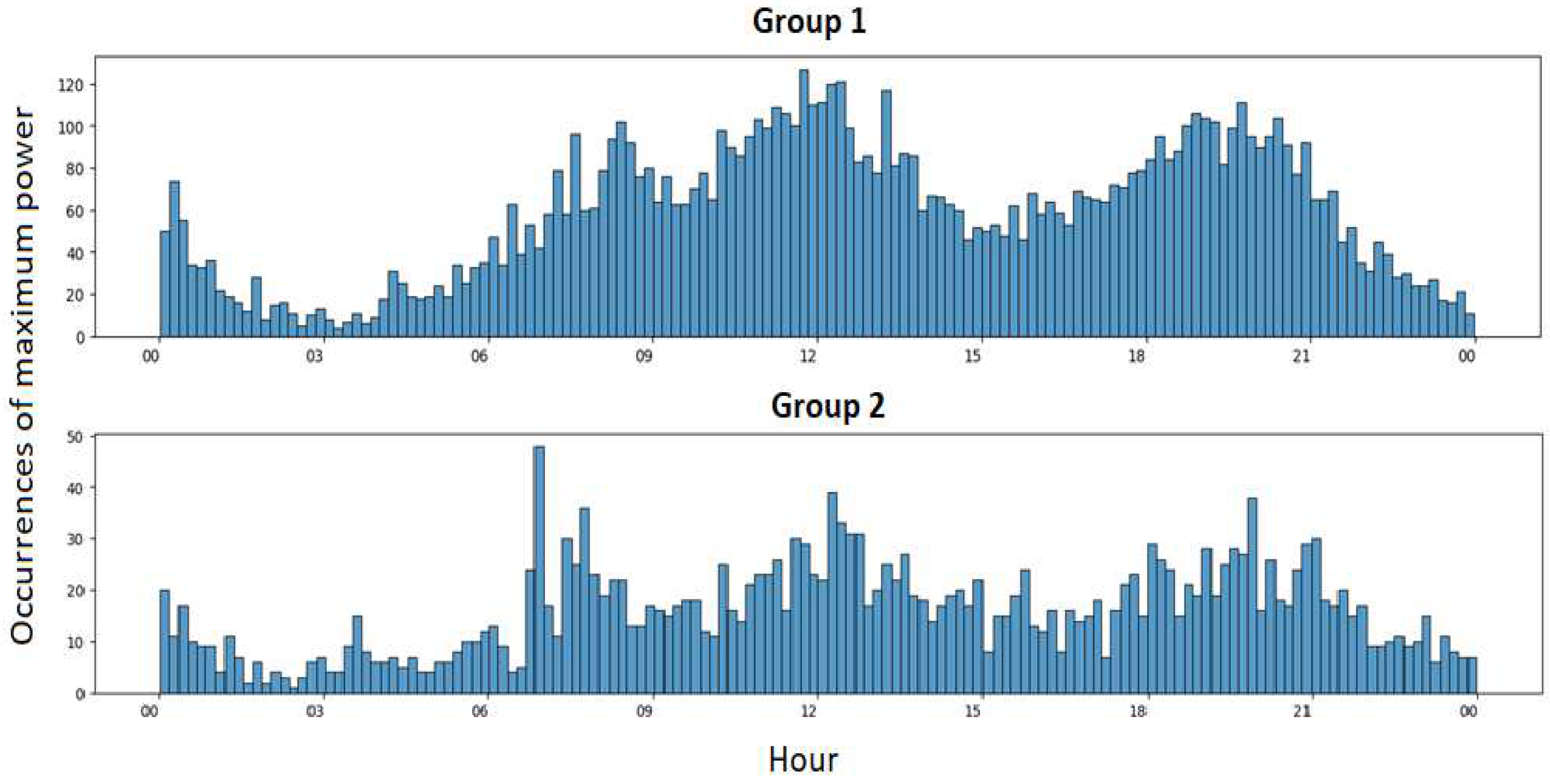
It can be observed that each customer exhibits different consumption patterns, and they vary considerably throughout the season. This leads us to believe that observing a group of aggregated customers could reveal patterns that are easier to identify. Figure 4 shows the occurrence of maximum power throughout the winter season for two different groups of customers. Group 1 consists of 70 consumers, and group 2 has 25. They are presented in Figure 4 through a histogram where each bar corresponds to a 10-minute interval that measures the occurrences of maximum power capture by Linky infrastructure.

Observing the occurrences by group makes the trends more apparent. For group 1, four concentrations of maximum power occurrences can be noted: around noon, 8 pm, 8 am, and midnight. For group 2, there is a significant concentration at 7 am and less pronounced concentrations around noon and 8 am. As the previous stage of disaggregation segments the customers from the secondary substation, we will have formed the groups of customers to analyze. Now, it is necessary to translate this information into adjusting the parameters of our function.

The concentrations of maximum power at a given period indicate whether it's a significant time for the cluster, deserving high resolution to finely adjust the peaks. Therefore, for each cluster, we can say that the most pronounced concentrations in the histograms will indicate the maximum number of Gaussians as well as the initial value of the "b" parameter for each of these Gaussians. To identify these concentrations, the “find_peaks” function from the Python SciPy library was used [39]. It allows for the identification and localization of local maxima in a one-dimensional dataset by simple comparison of neighboring values. The times of maxima will be denoted by the letter t, and the heights at which they appear will be denoted as

h_{t}

. This guides us towards another way of expressing our sum of Gaussians function f(x, a, b, c) and adjusting the parameter bounds. For each cluster k, we will have T numbers of Gaussians found from the histogram of maximum power occurrences, as indicated by Equation 4.

f (x, a, b, c) = \sum_{k = 1}^{K} \sum_{t = 1}^{T} (a_{t, k} * {e x p}^{\frac{{- (x - b_{t, k})}^{2}}{{2 * c}_{t, k}^{2}}}) 0 \leq a_{t, k} < \max (S e c o n d a r y S u b s t a t i o n C u r v e) h_{t} - 0.5 h o u r s \leq b_{t, k} \leq h_{t} + 0.5 h o u r s 1 h o u r < c_{t, k} < 6 h o u r s

(4)

Having the parameter

a_{t, k}

presenting a possible value of zero allows the optimization to discard the Gaussian (t,k) if it is not significant for curve fitting, setting its height to zero. This accounts for the variable behavior indicating that customers in this group may not have their maximum power at that time every day. The parameter

b_{t, k}

capable of varying by about half an hour around the time

h_{t}

, allows for moving the center of the Gaussian, which aligns with the occurrences of maximum power around each maximum. The parameter

c_{t, k}

represents the width of the Gaussian, with the lower bound set to one hour. This prevents the presence of peaks that appear and disappear very quickly, as we assume that the consumption of the customer group has some inertia in its variations. The upper bound for the

c_{t, k}

parameter is limited to 6 hours to avoid losing information about a possible important peak.

2.3. Global Vision of the Model

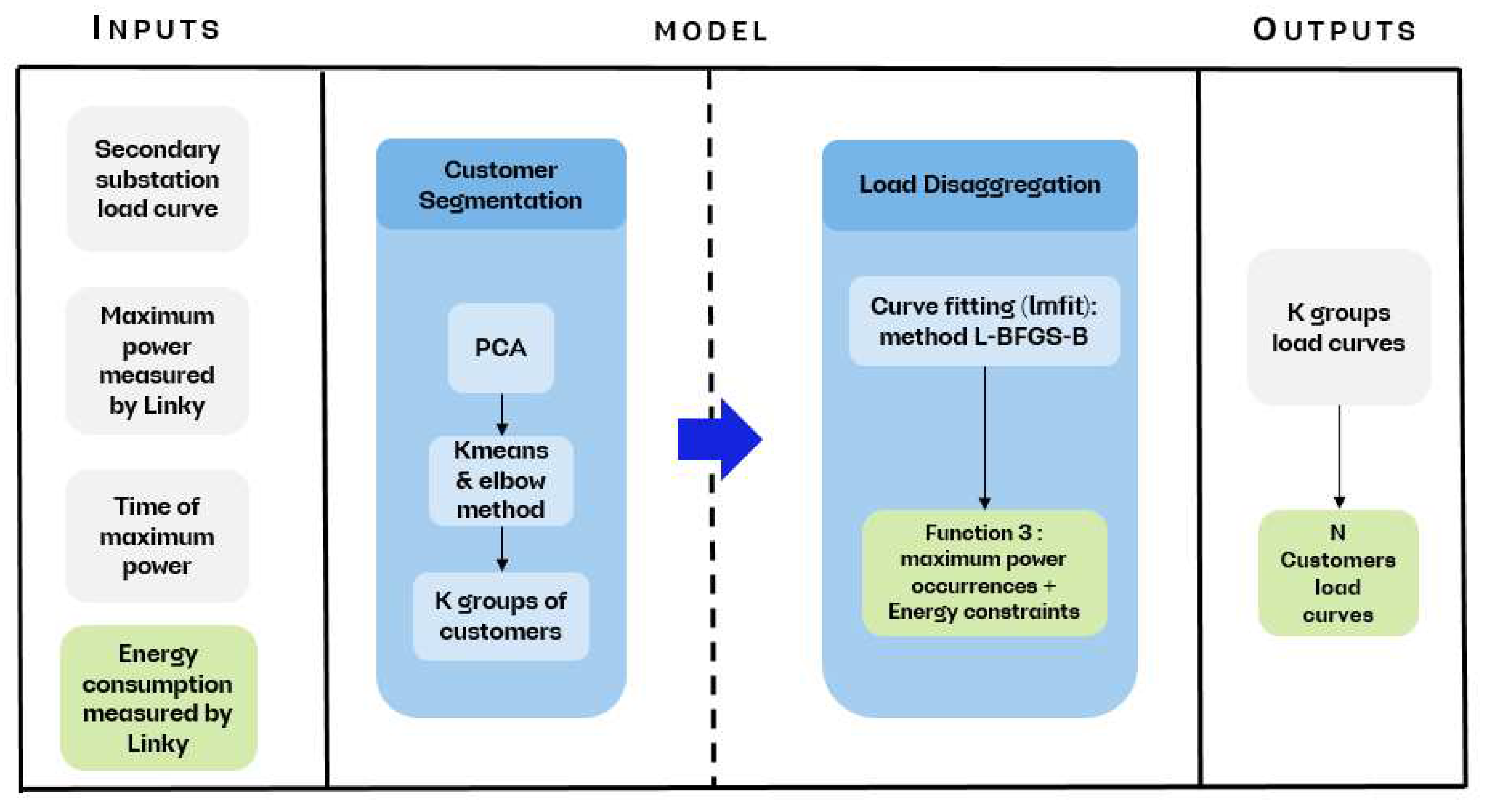
To facilitate the overall view of the model, a schematic gathering all its stages is presented in Figure 5.

2.4. Error Evaluation

The error produced by the model is calculated using symmetric mean average percentage error (SMAPE). SMAPE is a commonly used metric to assess the accuracy of forecasts or prediction models. It calculates the accuracy of predictions by comparing actual and predicted values in a symmetric way, as shown in the Equation 5:

S M A P E = \frac{1}{N} \times \sum_{n = 1}^{N} \frac{|P_{n} - R_{n}|}{\frac{(|R_{n}| + |P_{n}|)}{2}}

(5)

Where P is the predicted value and R is the real value. So, for each data point, it takes the absolute difference between the actual value and the predicted value, and then divides it by the sum of the actual and predicted values. SMAPE is robust to small values. Due to its symmetry, SMAPE ensures that the penalty for error is not sensitive to large differences between the prediction and the actual value.

With the help of SMAPE, we will evaluate the error between the reconstruction of the load curve of the secondary substation based on the model's result and the true load curve of the secondary substation. This way, we will be able to assess how well the disaggregation model can reconstruct the load curves of the secondary substation.

3. Results

The results of the disaggregation model are presented for both functions described in Section 2.2. The evaluation of the results for both models is conducted along two cases. On the first case, a random secondary substation is selected, and the model is applied to the load curve for the winter season. On the second case, the error is computed for all secondary substations on all days of the winter season.

3.1. Results for One Random Secondary Substation

A secondary substation was randomly chosen from the set of 48 in our dataset. This secondary substation has 198 connected consumers. The result of consumer segmentation, presented in 2.1, led us to the number K of similar customer groups equal to 6. The quantity of customers in each group can be observed in Table 1.

For each day of the winter season, our disaggregation model is put into practice using the two functions described in Section 2.2 and the 6 groups of customers. The results of the errors calculated are presented in Table 2.

In order to look at the load curves produced by the model with both functions, the days with minimal SMAPE error are select. These curves are illustrated by the Figure 6.

The individual load profiles of each cluster are presented by below. The individual load profiles produced by the model using function one and two are presented by Figure 7 and Figure 8 respectively.

3.2. Results for All Secondary Substation in the Dataset

For the 48 secondary substations, the total quantity of groups obtained by the segmentation step is presented in Table 3.

For each day of the winter season, our disaggregation model is put into practice using the two functions described in Section 2.2. The results of the errors calculated using SMAPE are presented in Table 4.

In order to look at the load curves produced by the model with both functions, the days for the secondary substations with minimal SMAPE error are selected. These curves are illustrated by the following Figure 7.

Figure 9. (a) Minimum SMAPE result produced by the model using function one; (b) Minimum SMAPE result produced by the model using function two.

4. Discussion

The results show us that the disaggregation model using function 2 presents better outcomes, even though function 2 has fewer degrees of freedom than function 1. If we look closely at the results with both functions for one random secondary substation, we can observe that function 1, purely mathematical, manages to capture the large peaks and valleys of the load curve, as shown in Figure 6a. However, it fails to capture the secondary peaks, thus leaving the curve fitting result unsatisfactory. On the other hand, function 2 incorporates characteristics of customer consumption into the modeling, thanks to the data from Linky meters. The interest in considering the behavior of customers from the segmentation step is to ensure consistency with reality, thus bringing the model closer to what happens in the network. It can be observed in Figure 6b that the fitted curve has successfully captured the various consumption peaks represented by the secondary substation load curve. This result is reflected in the shapes of individual profiles, as shown in Figure 8. This highlights the consistency between the distribution of maximum power occurrences per group of customers and the consumption measurements of all customers observed by secondary substation load curve. This is reflected when comparing the errors of the functions. The error produced by function 2 is lower than that of function 1 as shown in Table 2.

The result obtained for a random secondary substation holds when we look at all the substations in our dataset. As presented in Table 4, function 2 produces results with lower errors than function 1. This assures us of the importance of the maximum power information measured by the Linky meter. Additionally, it underscores the significance of data measured by smart meters for network load modeling.

5. Conclusion and Perspectives

We have decided to reverse the natural process, which involves starting from the development of aggregated customer curves to obtain an estimate of the secondary substation load curve. By leveraging the richness of Linky meter data, we have created a way to disaggregate the substation curve from this measurement into customer profiles. Developing an estimation methodology based on data measured by smart meters allows us to better estimate customer’s consumption behavior and its changes. This is crucial in the context of integrating new uses of the grid, such as renewable energy sources and electric vehicles. Unlike classical "bottom-up" methodologies that are highly dependent on measurements with fine temporal resolution, our developed methodology is based on the occurrence time of the maximum daily power. Additionally, our approach involves a disaggregation at a higher grid level, specifically the secondary substation level. This modeling idea is not discussed in the scientific literature, making this model innovative and potentially opening doors to considering how smart meter data can assist in network sizing, integrating new uses, and adapting to changes in consumer behavior in general.

The next stage of studying and improving the model involves exploring the energy measured by Linky meters in the disaggregation process. The evolution of the model can be added to the schematic seen in 2.3. This is presented in Figure 10.

Imposing an energy constraint ensures that our result, when viewed from the aggregate of customers, can be distributed to the entire customer base of each group while respecting their consumption. This will further bring the results closer to the reality of consumption in the network. This will allow us to transition from curves aggregated by consumer segments to curves of individual consumers, properly accounting for the energy consumed by them and measured by the Linky meter.

Author Contributions

Conceptualization, G.R.M.; methodology, G.R.M.; validation, G.R.M., C.G., M.C.H.A. and R.C.; formal analysis, G.R.M.; investigation, G.R.M.; resources, G.R.M.; data curation, G.R.M. and C.G.; writing—original draft preparation, G.R.M.; writing—review and editing, C.G., M.C.H.A. and R.C.; visualization, C.G., M.C.H.A. and R.C.; supervision, C.G., M.C.H.A. and R.C..; project administration, C.G. and R.C.; funding acquisition, R.C.. All authors have read and agreed to the published version of the manuscript.

Funding

This study is part of a thesis work on the use of Linky smart meter data to improve load knowledge in LV grids. The work is funded by Enedis as part of the SmartGrids Chair of Grenoble INP Fondation and the MIAI Institute: ANR project 3IA MIAI@Grenoble Alpes.

Data Availability Statement

The datasets presented in this article are not available because of GDPR. They are associated with a customer panel, who have given their consent to Enedis for the use of their data in the context of Enedis network studies.

Conflicts of Interest

The authors declare no conflicts of interest.

References

European Commission. "‘Fit for 55’: delivering the EU’s 2030 climate target on the way to climate neutrality." Communication from the Commission to the European Parliament, the European Council, the Council, the European Economic and Social Committee and the Committee of the Regions (2021).
Open Data Enedis. (n.d.) Enedis. Available online: https://data.enedis.fr/pages/accueil.
Consommation d’énergie par usage du résidentiel. (n.d.). Données Et Études Statistiques Pour Le Changement Climatique, L’énergie, L’environnement, Le Logement Et Les Transports. Available online: https://www.statistiques.developpement-durable.gouv.fr/consommation-denergie-par-usage-duresidentiel.
Chudjakov, N. (2010). Enel: Italy reaping first-mover benefits of smart meters. www.euractiv.com. Available online: https://www.euractiv.com/section/climate-environment/interview/enel-italy-reaping-first-mover-benefits-of-smart-meters/.
The Circular Smart Meter: sustainable innovation by Enel. (2022, March 29). Available online: https://www.enel.com/company/stories/articles/2022/03/circular-smart-meter-regenerated-plastic.
SmartMeter FAQ. | PG&E (n.d.). Available online: https://www.pge.com/en_US/residential/save-energy-money/analyze-your-usage/your-usage/view-and-share-your-data-with-smartmeter/smartmeter-faq.page.
Smart Metering & Infrastructure Program Business Case | BC Hydro (n.d.). Available online: https://www.bchydro.com/content/dam/BCHydro/customer-portal/documents/projects/smart-metering/smi-program-business-case.pdf.
M. Jensterle, “System integration of renewables and smart grids in Korea : supporting Germany’s energy dialogue with Japan and Korea ; short scientific report,” 2019. Available online: https://nbn-resolving.org/urn:nbn:de:bsz:wup4-opus-74320.
Smart Meter Project | TEPCO. (n.d.). Available online: https://www.tepco.co.jp/en/pg/development/domestic/smartmeter-e.html.
La CRE : favorable à la généralisation du compteur Linky. (n.d.). CRE. Available online: https://www.cre.fr/documents/Presse/Communiques-de-presse/la-cre-favorable-a-la-generalisation-du-compteur-linky.
Thibaut Barbier. Modélisation de la consommation électrique à partir de grandes masses de données pour la simulation des alternatives énergétiques du futur. Energie électrique. Université Paris sciences et lettres, 2017. Français.
L. Suganthi and A. A. Samuel, “Energy models for demand forecasting—A review,” Renewable & Sustainable Energy Reviews, vol. 16, no. 2, pp. 1223–1240, Feb. 2012. [CrossRef]
Z. Shao, C. Fu, S. Yang, and K. Zhou, “A review of the decomposition methodology for extracting and identifying the fluctuation characteristics in electricity demand forecasting,” Renewable & Sustainable Energy Reviews, vol. 75, pp. 123–136, Aug. 2017. [CrossRef]
J. Runge and R. Zmeureanu, “Forecasting Energy use in buildings Using Artificial Neural Networks: A review,” Energies, vol. 12, no. 17, p. 3254, Aug. 2019. [CrossRef]
L. G. Swan and V. I. Ugursal, “Modeling of end-use energy consumption in the residential sector: A review of modeling techniques,” Renewable & Sustainable Energy Reviews, vol. 13, no. 8, pp. 1819–1835, Oct. 2009. [CrossRef]
K. Zhou, S. Yang, and C. Shen, “A review of electric load classification in smart grid environment,” Renewable & Sustainable Energy Reviews, vol. 24, pp. 103–110, Aug. 2013. [CrossRef]
M. Tureczek, P. S. Nielsen, and H. Madsen, “Electricity consumption clustering using smart meter data,” Energies, vol. 11, no. 4, p. 859, Apr. 2018. [CrossRef]
T. Räsänen, D. Voukantsis, H. Niska, K. Karatzas, and M. Kolehmainen, “Data-based method for creating electricity use load profiles using large amount of customer-specific hourly measured electricity use data,” Applied Energy, vol. 87, no. 11, pp. 3538–3545, Nov. 2010. [CrossRef]
RTE. Consommation française d’électricité : Caractéristiques et methods de prévision. Techical report, RTE, November 2014.
Grandjean, J. Adnot, and G. Binet, “A review and an analysis of the residential electric load curve models”, Renewable and Sustainable Energy Reviews, 2012. [CrossRef]
R. Bartels, D. G. Fiebig, M. Garben, and R. Lumsdaine, “An end-use electricity load simulation model”, Utilities Policy, 2(1) :71 – 82, 1992. [CrossRef]
B. Gao, X. Liu, and Z. Zhu, “A Bottom-Up model for household load profile based on the consumption behavior of residents,” Energies, vol. 11, no. 8, p. 2112, Aug. 2018. [CrossRef]
K. Gajowniczek and T. Ząbkowski, “Short term electricity forecasting using individual smart meter data,” Procedia Computer Science, vol. 35, pp. 589–597, Jan. 2014. [CrossRef]
Estebsari and R. Rajabi, “Single residential load forecasting using deep learning and image encoding techniques,” Electronics, vol. 9, no. 1, p. 68, Jan. 2020. [CrossRef]
R. A. Sevlian and R. Rajagopal, "A model for the effect of aggregation on short term load forecasting," 2014 IEEE PES General Meeting | Conference & Exposition, National Harbor, MD, USA, 2014, pp. 1–5. [CrossRef]
Zoha, A. Gluhak, M. A. Imran, and S. Rajasegarar, “Non-Intrusive Load Monitoring Approaches for Disaggregated Energy Sensing: a survey,” Sensors, vol. 12, no. 12, pp. 16838–16866, Dec. 2012. [CrossRef]
Y. F. Wong, Y. Ahmet Şekercioğlu, T. Drummond and V. S. Wong, "Recent approaches to non-intrusive load monitoring techniques in residential settings," 2013 IEEE Computational Intelligence Applications in Smart Grid (CIASG), Singapore, 2013, pp. 73–79. [CrossRef]
S. S. Hosseini, K. Agbossou, S. Kélouwani, and A. Cardenas, “Non-intrusive load monitoring through home energy management systems: A comprehensive review,” Renewable & Sustainable Energy Reviews, vol. 79, pp. 1266–1274, Nov. 2017. [CrossRef]
R. Bro and A. K. Smilde, 2014, “Principal component analysis” Analytical methods, 2812-2831. [CrossRef]
J. Hartigan and M. A. Wong, “Algorithm AS 136: A K-Means Clustering Algorithm,” Applied Statistics, vol. 28, no. 1, p. 100, Jan. 1979. [CrossRef]
Likas, A., Vlassis, N., & Verbeek, J. (2003). The global k-means clustering algorithm. Pattern Recognition, 36(2), 451–461. [CrossRef]
M. A. Syakur, B. K. Khotimah, E. M. S. Rochman, and B. D. Satoto, “Integration K-Means Clustering Method and Elbow Method For Identification of The Best Customer Profile Cluster,” IOP Conference Series: Materials Science and Engineering, vol. 336, p. 012017, Apr. 2018. [CrossRef]
Finding a “Kneedle” in a Haystack: Detecting Knee Points in System Behavior Ville Satopa † , Jeannie Albrecht† , David Irwin‡ , and Barath Raghavan§ †Williams College, Williamstown, MA ‡University of Massachusetts Amherst, Amherst, MA § International Computer Science Institute, Berkeley, CA.
E. C. Levy, "Complex-curve fitting," in IRE Transactions on Automatic Control, vol. AC-4, no. 1, pp. 37–43, May 1959. [CrossRef]
M. Newville, A. Ingargiola, T. Stensitzki, and D. B. Allen, “LMFIT: Non-Linear Least-Square Minimization and Curve-Fitting for Python,” Astrophysics Source Code Library, Sep. 2014. [CrossRef]
R. H. Byrd, P. Lu, J. Nocedal, and C. Zhu, “A limited memory algorithm for bound constrained optimization,” SIAM J. Sci. Comput., vol.16, no. 5, pp. 1190–1208, Sept. 1995. [CrossRef]
“Reconstituer les flux de responsabilité d’équilibre - RTE Portail Services,” Portail Services RTE. Available online: https://www.services-rte.com/fr/decouvrez-nos-offres-de-services/le-role-des-gestionnaires-de-res/reconstituez-les-flux-re.html.
Enedis, « Règles de gestion mises en oeuvre par Enedis pour le traitement des données dans le processus de Reconstitution des Flux ». Disponible :. Available online: https://www.enedis.fr/sites/default/files/import/Enedis-NOI-CF_103E.pdf.
Scipy.Signal.find_Peaks — SciPy v1.11.3 Manual. (n.d.). Available online: https://docs.scipy.org/doc/scipy/reference/generated/scipy.signal.find_peaks.html.

Figure 1. Example of obtaining profiles at the customer level from the disaggregation model.

Figure 2. Customer segmentation steps.

Figure 3. Occurrences of maximum power for five customers during the days in winter season.

Figure 4. Occurrences of maximum power for all customers of each group during the winter season.

Figure 5. Schematic of the disaggregation model.

Figure 6. (a) Minimum SMAPE result produced by the model using function one; (b) Minimum SMAPE result produced by the model using function two.

Figure 7. The individual load profiles of each cluster produced by the model using function one.

Figure 8. The individual load profiles of each cluster produced by the model using function two.

Figure 10. Schematic of the disaggregation model with the perspectives.

Table 1. Number of customers per group after the segmentation step.

Group	0	1	2	3	4	5
Customers	72	74	5	3	24	20

Table 2. SMAPE errors of the curve fitting for the winter season.

SMAPE	Function1	Function 2
Minimal (%)	4.09	1.60
Mean (%)	6.36	2.64
Maximum (%)	10.81	3.99

Table 3. Number of secondary substations per quantity of groups after the segmentation step.

Quantity of Groups	4	5	6	7
Number of Substations	4	23	16	5

Table 4. Mean SMAPE errors of the curve fitting for all secondary substations in winter season.

SMAPE	Function1	Function 2
Minimal (%)	8.43	2.93
Mean (%)	17.86	4.91
Maximum (%)	60.15	7.08

Disclaimer/Publisher’s Note: The statements, opinions and data contained in all publications are solely those of the individual author(s) and contributor(s) and not of MDPI and/or the editor(s). MDPI and/or the editor(s) disclaim responsibility for any injury to people or property resulting from any ideas, methods, instructions or products referred to in the content.

© 2024 by the authors. Licensee MDPI, Basel, Switzerland. This article is an open access article distributed under the terms and conditions of the Creative Commons Attribution (CC BY) license (http://creativecommons.org/licenses/by/4.0/).

Copyright: This open access article is published under a Creative Commons CC BY 4.0 license, which permit the free download, distribution, and reuse, provided that the author and preprint are cited in any reuse.

MDPI Initiatives

Important Links

Choose an area of interest and we will send you notifications of new preprints at your preferred frequency.

Disclaimer