Submitted:
07 February 2024
Posted:
08 February 2024
You are already at the latest version
Abstract
Wireless Sensor Networks are critical for modern applications ranging from environmental monitoring to smart city infrastructures. This research proposes a novel optimization learning and deployment strategy for Wireless Sensor Networks (WSNs) by 3D WUSN model is uniformly distributed M sensor nodes across diverse terrains, with clusters representing 20% of sensors, showcasing its ability to balance power consumption and extend network longevity, grounded in fuzzy clustering based protocol using the Fuzzy C-Means (FCM) method, called FCM-3DWUSN. Comparative analysis against established models including LEACH-C, K-Means and LEACH emphasized FCM-3DWUSN's outperformed performance, with average power consumption such as 134.990, 341.790, 143.895, and 192.984; respectively. The experimental result shows that FCM protocol in the 3D WUSN model can reduce energy consumption and improve the network lifetime to gather data and send the information.
Keywords:
Wireless sensor networks
; FCM-3WUSN clustering algorithm
; Routing algorithm
; Power load balancing
; Optimization learning.
1. Introduction
Wireless Sensor Networks (WSNs) have emerged as necessary tools across the spectrum of applications, ranging from environmental surveillance to the foundational blocks of smart city infrastructures. Their ubiquity is not just a testament to their versatility but also heralds the advent of an interconnected future. As we increasingly integrate WSNs into the fabric of our daily lives, they simultaneously open doors to new possibilities and present multifaceted challenges.
Foremost among these challenges is the complicated management of power resources. Within the vast and interconnected maze that constitutes Wireless Sensor Networks, optimal power distribution and consumption become central. This not only ensures the prolonged viability of each node but is also paramount for the longevity and reliability of the entire network.
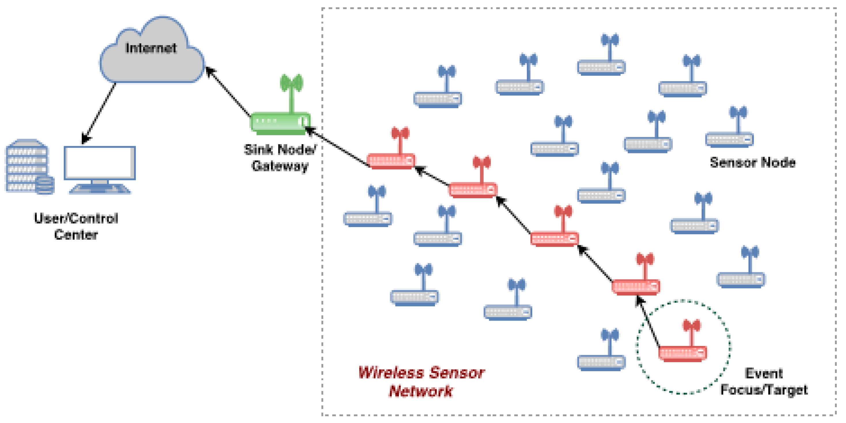
In the realm of environmental monitoring, Wireless Sensor Networks have particularly showcased their prowess. Comprising small, energy-efficient devices, these networks are adept at collecting and wirelessly transmitting data from diverse environments to a central node or base station (BS). Their capability to relay real-time, comprehensive data, even from remote and inaccessible terrains, marks a significant leap over traditional monitoring techniques. This evolution translates to not only enhanced accuracy but also substantial cost efficiencies, given the reduced human intervention and maintenance resources.
Wireless Sensor Networks, specially tailored for environmental metrics, seamlessly integrate three core components: sensing nodes strategically dispersed in the monitoring environment, a base station entrusted with data collation and processing, and a robust communication protocol to ensure unhindered data flow between nodes and the base station.
Their transformative impact is further underscored by their wide-ranging applications, spanning from tracking forest fires to real-time wildlife movements. As we continue to push the boundaries of technological innovation, WSNs are positioned to become even more integral to environmental conservation and management.
The LEACH algorithm (Low Energy Adaptive Clustering Hierarchy) [1] is one of the pillars underpinning the efficiency of Wireless Sensor Networks. Designed with a focus on clustering, LEACH’s primary objective is to extend the network’s functional life by judiciously managing power during data aggregation phases. By designating specific nodes as cluster heads for data relay, LEACH minimizes energy-intensive long-range communications to the BS. Such foundational strategies of LEACH have been the springboard for numerous iterations and enhancements, each striving for a delicate balance between power efficiency and cluster-centric communication.
Building on the LEACH foundation, LEACH-C (Centralized LEACH) [1] integrates a centralized base station to further refine the efficiency and scalability of Wireless Sensor Networks. By centralizing data acquisition and leveraging the holistic view of the network that the base station provides, LEACH-C enhances decision-making and network performance metrics. While centralization offers a myriad of advantages, it also poses challenges, especially in ensuring synchronized communication between the central base and peripheral nodes. However, these challenges have been meticulously addressed, ensuring that LEACH-C remains a robust and streamlined architecture in Wireless Sensor Networks.
The sphere of Wireless Sensor Networks has also witnessed a surge in the exploration of load-balancing techniques. These methods, tailored for WSN longevity, primarily focus on adaptive strategies. By dynamically modulating cluster sizes based on factors like residual power and network traffic, these techniques have consistently showcased superior performance metrics against their traditional counterparts. This forward momentum in load-balancing innovations provides a promising trajectory for the future landscape of Wireless Sensor Networks.
Another key contributor to the evolving clustering algorithm narrative is the Fuzzy C-Means (FCM) [1]. An extension of the K-means algorithm, FCM introduces nuanced soft assignments. In FCM’s paradigm, data points are not rigidly tethered to a specific cluster. Instead, they possess membership values, providing a gradient of association across multiple clusters. This complicated layering proves invaluable when the data landscape is riddled with ambiguities or has significant cluster overlaps.
To achieve energy efficiency in WSN, several models have been done.
D. C. Hoang et al. [1] presented and analyzed a cluster-based protocol using the Fuzzy C-Mean (FCM) method to reduce energy consumption within the Wireless Sensor Network to improve the network life. This protocol applied the FCM algorithm to create a cluster structure that minimizes the spatial distance between sensor nodes and thus creates a better cluster obtain formation. With support for data aggregation, cluster head rotation, and intra-cluster TDMA scheduling techniques, energy consumption is balanced among all sensor nodes and the amount of data transmitted to the BS is significantly reduced.
M. Baghouri et al. [2] presented a difference between two dimensions (2D) and three-dimensional (3D) configuration of Wireless Sensor Network (WSN). Furthermore, WSN is known as a technology applied in everyday life, however, the analysis of 3D WSN is more complex than the analysis of 2D WSN. In this work, they showed that this approximation is not valid if the height of the network is larger than the length and width of this network, and power consumption and throughput in 3D environments are significantly reduced compared to 2D. Their experimental results showed that the 2D approximation was not reasonable because the lifetime of 3D WSN was reduced by about 21% compared to 2D WSN by the LEACH protocol. Their limitations exist for optimizing the energy consumption of this network, but it will be done considering that the number of cluster heads in 3D WSN yields more results than in 2D WSN.
Other authors [3] propose an optimization based on energy-efficient routing protocol based on multi-threshold segmentation (named EERPMS) in Wireless Sensor Network to improve the distribution uniformity of cluster heads, prolong, and save network energy through comparison of protocols.
T. H. Dang et al. [4] explored the machine learning techniques for classical learning such as Fuzzy C-Means (FCM) [1], K Means, … in 3D WSN. They proposed an efficient topology in a 3D Wireless Sensor Network (3D WSN) that balances node energy consumption, improves the capability of data transmission and prolongs network life. The proposed FCM-PSOEB method aims to create 3 steps as: firstly, creates energy-efficient clusters consisting of cluster heads (CHs) and cluster members (non-CHs) using the Fuzzy C-Means algorithm. Secondly, particle cluster optimization is used to find the optimal CH to reduce the number of network disconnections from existing clusters. Finally, the process assigns non-CHs to the most suitable clusters to ensure load-balancing between clusters. D. T. Hai et al. [6] used a Lagrange multiplier method, the solutions of the model including cluster centers and membership matrices are calculated and used in the Fuzzy C-Means algorithm called FCM-3WSN by a mathematical model for clustering in 3D WSN, considering energy consumption, communication constraints and 3D energy function.
Other authors [7,8,9] showed various machine learning techniques suitable for energy-efficient routing using WSN. Furthermore, other researchers [9,10,11,12] propose current SDN or IoT trending technology uses Wireless Sensor Network.
The structure of this paper consists of 5 sections. Section 1 introduces the general management of Wireless Sensor Networks, an overview and some information about the clustering algorithm of the problem. Section 2 introduces the model and optimizes the model. Section 3 proposes an algorithm for the optimal model. In the remaining 2 parts, part 4 describes the experiment and concludes in section 5.
Motivations
The rapid proliferation and integration of Wireless Sensor Networks (WSNs) in everyday applications underscore an urgent need for enhanced performance and reliability. As these networks become the backbone of critical systems from environmental monitoring to the very fabric of smart cities, there is a pressing demand for optimization techniques that not only enhance data accuracy, but also ensure network functionality is maintained and efficient. Recognizing this, our motivation lies in bridging existing gaps, elevating WSNs’ capabilities and setting new benchmarks in energy efficiency and connectivity, thereby driving the evolution of WSNs to meet the rising challenges of the modern world.
Contributions
Amid the expanding applications of Wireless Sensor Networks (WSNs), achieving optimal performance is paramount. Our contributions address this by introducing advanced mechanisms and models, setting new benchmarks in power efficiency and connectivity within WSNs. The main contributions can be summarized as follows:
Optimization and Deployment for WSNs: We propose a comprehensive strategy for Wireless Sensor Networks (WSNs) targeting power efficiency, coverage, connectivity, and data reliability. Using varied deployment strategies ensures seamless, high-quality coverage with minimal sensor node installations across applications from environmental sensing to smart cities.
FCM-3DWUSN technique: We propose a new technique as the foundation for fuzzy clustering and particle swarm optimization, which outperforms established algorithms. Alongside this, we have presented a novel 3D WUSN model with uniformly distributed M sensor nodes, ensuring consistent and broad data collection, named FCM-3DWUSN.
Advanced Cluster Mechanism and Communication Protocol: Established a structure where ground nodes have dual roles and facilitate systematic hourly data transmission to BS. This is coupled with efficient one-hop communication between cluster members and Cluster Heads, a centralized permanent base station for consistent data aggregation, and an adaptive rotation mechanism for Cluster Heads based on residual power, ensuring sustained network efficiency.
The research amalgamates advanced techniques and systematic methodologies, paving the way for optimizing Wireless Sensor Networks in varied applications.
2. System Model
2.1. 3D WUSN Model
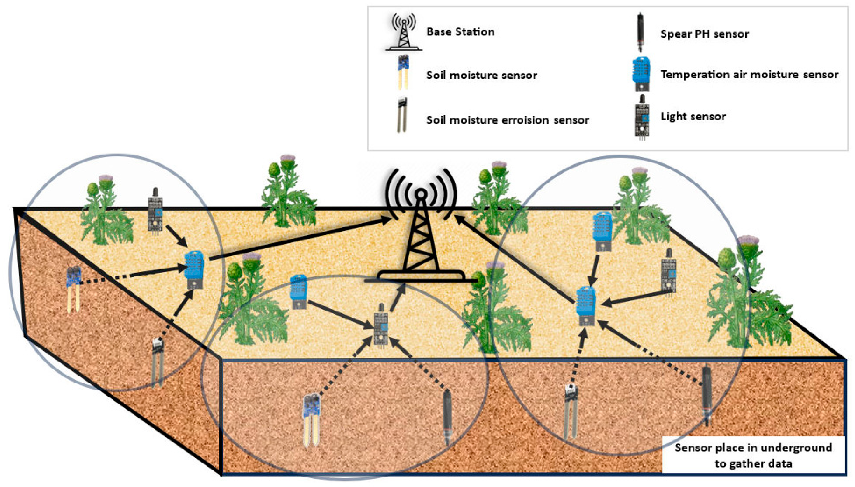
We propose a 3D WUSN system with M sensors [1-2-3-4]. These sensors are spread out evenly on the ground, each having a specific job based on where they are and what they do. This setup ensures full coverage and good data collection. Here are the main ideas guiding this setup:
- -
- After setting them up, all sensors stay put. Even though they have different jobs, they all start with the same amount of power and keep it consistent.
- -
- There are an equal number of sensors on the ground and below it. In each group or “cluster” (let’s call C), there’s an even mix of M sensors.
- -
- Sensors on the ground can either be leaders (Cluster Heads or CH) or just regular members. Only the leader sensor collects data from both on-the-ground and underground sensors, sending it to the Base Station (BS) every hour.
- -
- Within each group, some sensors, marked as k, focus mainly on collecting data. They then send this data to their leader sensors above the ground.
- -
- For communication, sensors talk directly to their leader sensors. These leader sensors then send data to the main control point without any stops in between.
- -
- The main control point, crucial for putting all data together, is always fixed in one central spot.
- -
- At the end of each hour of communication, we check how much power each sensor has left. This helps us decide if we need to change the leader sensors.
In short, this setup, based on the points above, helps us collect data in the best way while saving as much power as possible in our sensor network.
Figure 1.
The WUSN Model.
2.2. Mathematical Model
We assume a 3D WUSN model where M sensor nodes are in the field. They are distributed on the ground to collect information. They are fixed in locations and uniformly distributed in configuration and function. Sensors are placed in coverage with each other. Some assumptions are made as follows:
- -
- All sensor nodes are fixed after being deployed, and the energy of the nodes is the same at the beginning, although in the model the sensors are used for different purposes, and their energy is the same at initialization.
- -
- M sensor nodes will be assigned to a given cluster C. The number of nodes above the ground and underground was divided based on the ratio of the datasets.
- -
- The number of members in clusters is not the same quantity.
- -
- Nodes marked as CH will be on the ground, and a cluster will form between the above-the-ground and underground nodes. The nodes that are above the ground, can be designated as member nodes or can be cluster heads if it is a cluster head, then it will collect information from underground and above the ground nodes which transmits the information to the BS. The transmission schedule will be 1 hour each.
- -
- In a cluster, there will be k underground nodes, the underground nodes are responsible for collecting and transmitting information to the CH node on the ground.
- -
- Single-hop communication is assumed in the sense that member clusters to CH directly and CHs forward data to BS in the communication range.
- -
- The BS will be permanently assigned in a central location.
- -
- After each round, all nodes will be calculated with the remaining energy so that BS would consider updating the array nodes for the next rounds based on the remaining energy.
Figure 2.
The overview of the proposed network model.
This study is motivated based on the model, then we deliver the new model combining those above assumptions. Sensors have limited power (mainly battery-powered) and processing capabilities. Sensing and processing require energy-intensive processes, specifically including environmental sensing components, data aggregation, and data transmission and reception [4-9]. The energy consumed in the transmission of l-bit data [9] at the distance (d) is represented [3] by ECM−CH and it is calculated in Equation (1). If d ≤ dth in which dth is the constant of the distance, energy consumption is calculated based on the free space model with d2. Conversely, it is the multi-path fading model with d4 energy dissipation. The energy consumption of a sensor in the cluster is given by the formula below.
where is the number of data bits and be energy consumption per bit to run the transmitter or the receiver data. be the energy required for amplifying mode, and be the distance from CM to CH [4]. be the location of CH of clusters, and be the location of sensor nodes. The formula for calculating the energy consumption of a CH for assembling data and transferring it to BS is as follows:
where be the energy consumption for data aggregation, be the energy loss by the amplifier mode [4], and be the distance from CH to BS [9] at a certain terrain [4-9]. be the location of BS. Hence the entire network has energy consumption [4] is as Equation (3):
The energy path loss from the underground nodes to above-the-ground CH is calculated according to the formula. When transmitting data from underground sensors to CH, the Friis model [5] is adopted to calculate the path loss, it is derived from the Friis equation in free space and is modified when electromagnetic waves are transmitted in sediments. The path loss quantifies the EM wave attenuation with the transmission distance. When the antenna gains are not included, then the path loss in free space can be simplified to Equation (4):
where be the distance between the sender sensor as the underground sensor and the received sensor as CH placed on the terrain. The distance could be calculated via the 3D Euclidean. Accordingly, will be the depth of node and be the height of node CH above the ground. Variants for underground are and are the constant of phase shifting and attenuation, respectively. Equation (4) is used to compute the energy of the path loss.
The Taylor series is used to expand the log function in Equation (5) into a polynomial function.
As per the above assumption, the network consists of k underground nodes. The CM-CH-BS nodes’ energy transmissions and the energy lost by the k nodes buried underground will make up the network’s total energy as Equation (8):
Combining Equations (3), and (8), we have the total energy model [4] of the network as follows:
From the energy model in Equation (9), we fuzzed them and proposed the mathematical model to minimize the total energy of the network as the Equation (10) below.
The clustering problem’s objective function is represented by Equation (10). The degree of belonging and the cluster center are the two primary factors that need to be assigned to cluster in this kind of situation. The problem’s objective is to distribute sensors among clusters [9], and then choose the cluster header. The data is passed directly from CM to CH and CH to BS. The BS would take into account re-clustering and re-selecting CH, depending on the remaining energy of the network’s sensors after each loop. Regarding the limitation of communication constraints, the following conditions are incorporated:
We have the new clustering model in equations (10-13). Before we state the new algorithm, we solve the optimization problem by the Lagrange multiplier method.
Where is the fuzzification coefficient (usually , is the number of clusters, is the number of sensors, and is the number of bits in each data packet. is the communication range, and is calculated by 3D Euclidean. The objective Equation (11) is a nonlinear optimization problem. Constraints (12) and (13) are given in the Wireless Sensor Networks problem to simulate the communication range between two normal sensor nodes, as well as from normal sensors to BS. Constraint (11) means that the membership of each sensor node in each cluster is represented to a degree as the membership function. The result of equations to calculate and is provided in Equations (14), and (15) below.
Since there is:
Denote from:
Figure 3.
The general process algorithm.
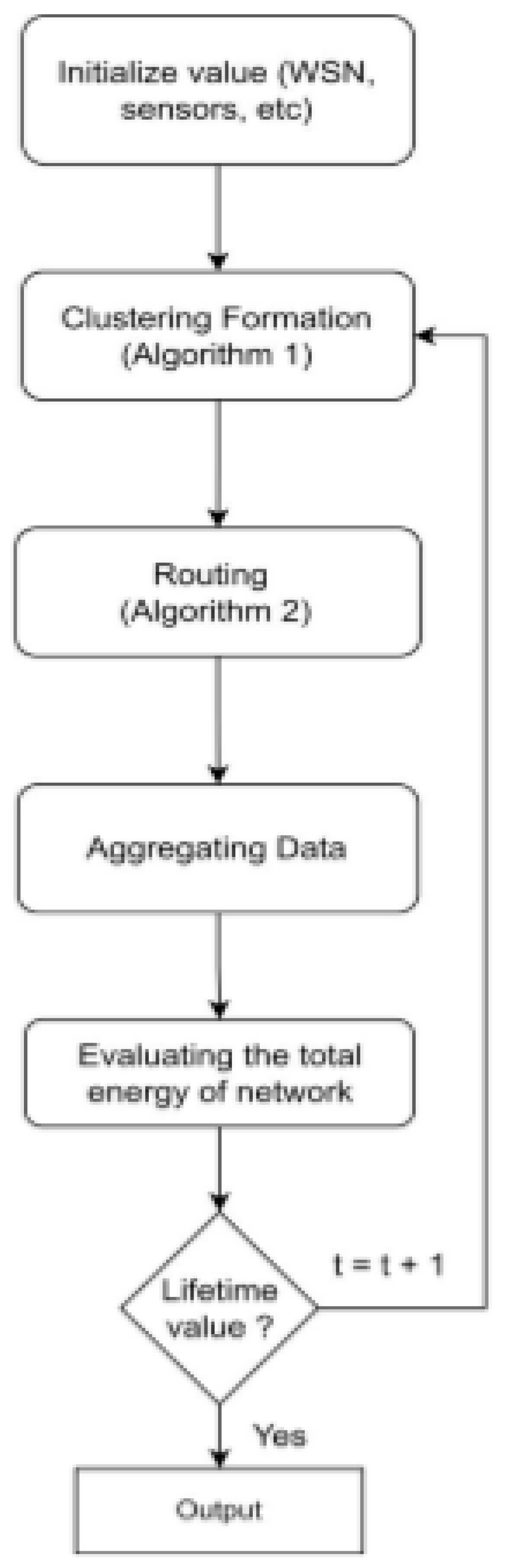
3. The FCM-WSN algorithm
From the solutions of the problem (11, 12, 14), we propose a better clustering algorithm named Fuzzy C-Means (FCM) [6] for 3D WUSN named FCM-3WUSN described in Algorithm 1. The purpose of extending the lifetime of the WUSN [9] is to optimize the energy consumption of the sensors in the local cluster and communicate with the CHs-BS. Therefore, sensors in a cluster transmit data to their CH node, and that CH node aggregates the data from the sensors, removes redundant information, and transmits them to BS [6]. Communication constraints are guaranteed during clustering. Thus power consumption for the transmission process is significantly reduced. The cluster-based routing protocol presented in this study for efficient routing in WUSN performs routing of packets collected by sensor nodes to cluster head (CH) nodes through cluster member nodes or directly [7]. The CH nodes forward directly to BS and maintain the route for efficient routing of data packets [7-9]. The routing algorithm describes how the database is derived from a cluster member to BS. The steps of the proposed routing algorithm are described below:
| Algorithm 1 FCM-3DWUSN Clustering formation | |
| Input: A number of sensors (M); A number of clusters (C); Fuzzifier; The maximum iteration maxSteps; Sensor list. Output: Matrix u, and a matrix of center V |
|
| 1: | t ← 0 |
| 2: | k ← 1 |
| 3: | Initialize ukj satisfied the equation (11). |
| 4: | while ||ut – ut–1|| > є do |
| 5: | t = t + 1 |
|
6: 7: |
Calculate V following the equation (19). Calculate u following the equation (18). |
| 8: | end while |
| 9: | while k < C do |
| 10: | if ( = min(Ɐi Ck) and then |
| 11: | i(CH) ← true |
| 12: | end if |
| 13: | if ( < Tr (Ɐi Ck) then |
| 14: | i(non – CH) ← true |
| 15: | end if |
| 16: | end while |
| Algorithm 2 Routing algorithm |
| Step 1: Reading the power levels and location (, yi, zi) of sensor nodes Si, i = 1, 2, 3, … |
| Step 2: Sending “HELLO” packet to all the neighbor nodes from a base station and find distances of node from a base station and between the nodes. |
| Step 3: At BS, the FCM-3DWUSN algorithm is used to select CH, and cluster it, based on distance and power of the nodes. |
| Step 4: Sending data from CMs to CH in each cluster. |
| Step 5: Accumulating data at BS. |
| Step 6: If power levels of at least 50% of nodes are drained. |
| Step 7a: If Step 6 yes: STOP. |
| Step 7b: If Step 6 no: check if CH rotation if it is needed. |
| Step 8: If yes, then return Step 3. If no, then return Step 4. |
4. Experiment
4.1. Testbed
4.2. Experimental Results
First, we measure the power efficiency of the models on different terrains for the ratio of CHs connected to BS with a number of clusters is 20% of a number of sensors. Table 2 gives the network energy consumption for specific models: FCM-3DWUSN, LEACH-C, LEACH and K-Means. Finally, FCM-3DWUSN requires the smallest average energy consumption compared to other models.
The graph in Figure 4 is shows the average value of the energy consumption of the algorithms with FCM-3DWUSN, LEACH-C, LEACH and K-Means are: 134.990, 341.790, 192.984 and 143.895; respectively. We find that FCM-3DWUSN obtained the best results.
Second, we compare several connections from CH to BS and from non-CH to CH. LEACH produces 100% of the CH-to-BS connection rate and 58.23% of the non-CH connection rate. On the contrary, the connection rates from non-CH to CH nodes of LEACH-C and K-means are very high: 100% and 98.84%, respectively, but CH to BS connection rates are quite low: 21.9% and 24.2%, respectively. Meantime, the connection rates from CHs to BS and from non-CHs to CH are high, obtaining 82.0% and 98.0%, respectively. In Figure 5, FCM-3DWUSN is shown to achieve the best results among all.
In Figure 6, we estimate the round (re-cluster) of every model. After each re-clustering, the CH of the clusters will be circulated to the sensors in the cluster [4,5,6,7,8,9,10]. Thereby, power consumption is balanced among sensors in the cluster and the network lifetime is extended. A number of FCM-3DWUSN rounds have the highest measurements, indicating that the power consumption is balanced among the clusters and prolongs the life of the Wireless Sensor Networks [10] in Figure 6 in the experiment.
5. Conclusions
In the rapidly evolving domain of Wireless Sensor Networks, achieving optimal performance remains both a challenge and a necessity, especially given the varied applications spanning from environmental sensing to smart city integration. Our study delved deep into this challenge, presenting a comprehensive strategy that significantly improves power efficiency, coverage, connectivity, and data reliability within WSNs. The introduction of the FCM-3DWUSN technique, rooted in fuzzy clustering and particle swarm optimization, has showcased its potential to outperform traditional algorithms like LEACH, LEACH-C, and K-Means. Our results, drawn from extensive experiments across diverse terrains, emphatically underscore FCM-3DWUSN’s capability to balance power consumption and extend the network’s lifespan [10,11,12].
Furthermore, our model’s adaptive nature, featuring an efficient one-hop communication protocol, and a systematic rotation mechanism for Cluster Heads based on residual power, promises sustained efficiency and adaptability. The results of this research not only set new benchmarks for Wireless Sensor Networks, but also offer a roadmap for future studies [11,12]. As technology continues to evolve, the strategies and methodologies presented in this paper will serve as a foundational guide, ensuring that Wireless Sensor Networks are not just efficient but also sustainable and adaptable to the ever-changing requirements of real-world applications.
In addition, it is recommended that researchers and the Wireless Sensor Networks community continuously conduct a number of future projects. Firstly, applying multi-hop among intra-cluster in the network, studying to deploy FCM-3DWUSN into smart agriculture applications to meet the requirements for solving problems in the real world, and studying to integrate meta-heuristic algorithms to optimize the energy consumption in WUSN could be considered as the improvement and developments from this research
Author Contributions
The authors confirm the contribution to the paper as follows: study conception and design: Dinh Phu Cuong Le, Dong Wang; data collection: Dinh Phu Cuong Le; analysis and interpretation of results: Dinh Phu Cuong Le, Dong Wang; draft manuscript preparation: Dinh Phu Cuong Le, Dong Wang and Nguyen Hoang Tu. All authors reviewed the results and approved the final version of the manuscript.
Funding
This work was supported in part by the National Natural Science Foundation of China under Grant 61502162, Grant 61702175, and Grant 61772184, in part by the Fund of the State Key Laboratory of Geoinformation Engineering under Grant SKLGIE2016-M-4-2, in part by the Hunan Natural Science Foundation of China under Grant 2018JJ2059, in part by the Key R & D Project of Hunan Province of China under Grant 2018GK2014, and in part by the Open Fund of the State Key Laboratory of Integrated Services Networks under Grant ISN17-14. Chinese Scholarship Council (CSC) through College of Computer Science and Electronic Engineering, Changsha 410082, Hunan University with grant CSC No. 2018GXZ020784.
Data Availability Statement
The data that support the findings of this study are available upon reasonable request to the authors.
Conflicts of Interest
The authors declare no conflicts of interest.
References
- Hoang, D. C.; Kumar, R.; Panda, S. K. Fuzzy C-Means Clustering Protocol for Wireless Sensor Networks. In Proceeding of 2010 IEEE International Symposium on Industrial Electronics (ISIE); 2010; pp. 3477–3482. [Google Scholar]
- Baghouri, M.; Hajraoui, A.; Chakkor, S. Low Energy Adaptive Clustering Hierarchy for Three-Dimensional Wireless Sensor Network. Recent Advances in Communications 2015, pp. 214–218. [Google Scholar]
- Yao, Y. D.; Li, X.; Cui, Y. P.; Wang, J. J.; Wang, C. Energy-Efficient Routing Protocol Based on Multi-Threshold Segmentation in Wireless Sensors Networks for Precision Agriculture. IEEE Sensors Journal 2022, 22, pp. 6216–6231. [Google Scholar] [CrossRef]
- Dang, T. H.; Nguyen, T. T.; Le, H. S.; Le, T. V. A Novel Energy-Balanced Unequal Fuzzy Clustering Algorithm for 3D Wireless Sensor Networks. In Proceedings of the 7th Symposium on Information and Communication Technology (SoICT ‘16). Association for Computing Machinery, New York, NY, USA; 2016; pp. 180–186. [Google Scholar]
- Abdorahimi, D; Sadeghioon, A.M. Comparison of Radio Frequency Path Loss Models in Soil for Wireless Underground Sensor Networks. Journal of Sensor and Actuator Networks 2019, 8, pp–35. [Google Scholar] [CrossRef]
- Hai, D. T.; Le Vinh, T. Novel Fuzzy Clustering Scheme for 3D Wireless Sensor Networks. Applied Soft Computing 2017, 54, pp.141–149. [Google Scholar] [CrossRef]
- Thangaramya, K.; Kulothungan, K.; Logambigai, R.; Selvi, M.; Ganapathy, S.; Kannan, A. Energy Aware Cluster and Neuro-Fuzzy Based Routing Algorithm for Wireless Sensor Networks in Iot. Computer Networks 2019, 151, pp.211–223. [Google Scholar] [CrossRef]
- Hou, R.; Fu, J.; Dong, M.; Ota, K.; Zeng, D. An Unequal Clustering Method Based on Particle Swarm Optimization in Underwater Acoustic Sensor Networks. IEEE Internet of Things Journal 2022, 9, pp. 25027–25036. [Google Scholar] [CrossRef]
- Singh, S.; Anand, V. Load Balancing Clustering and Routing for Iot-Enabled Wireless Sensor Networks. International Journal of Network Management 2023, 33, pp. e2244. [Google Scholar] [CrossRef]
- Luo, D.; Ren, C. A. Layered Routing Algorithm for Wireless Sensor Networks Based on Energy Balance. International Journal of Autonomous and Adaptive Communications Systems 2023, 16, pp. 141–158. [Google Scholar] [CrossRef]
- Devika, E.; Saravanan, A. A Survey of Node Localization in Wireless Sensor Networks Using Various Optimization Algorithms. In 2022 Third International Conference on Smart Technologies in Computing, Electrical and Electronics (ICSTCEE), IEEE, 2022, pp. 1-8.
- Qabouche, H.; Sahel, A.; Badri, A.; El Mourabit, I. Energy Efficient and Coverage Aware Grey Wolf Optimizer Based Clustering Process for Software-Defined Wireless Sensor Networks. Ad Hoc Networks 2023, 151, pp. 103288. [Google Scholar] [CrossRef]
Figure 4.
The average power consumption.
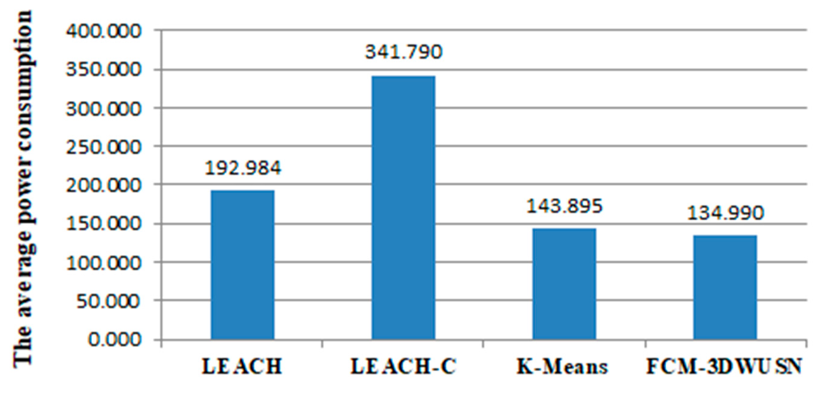
Figure 5.
The average of connections
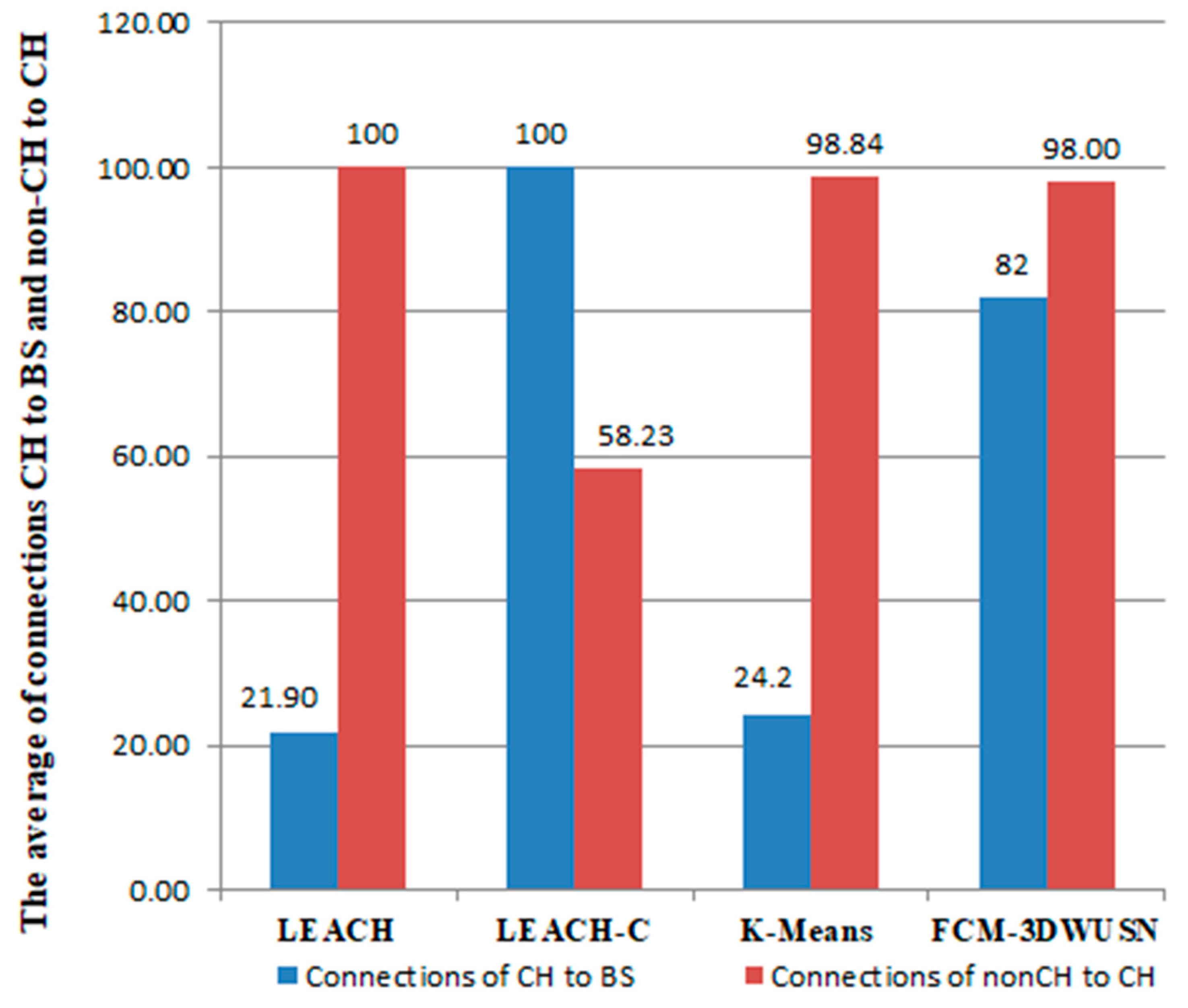
Figure 6.
The rounds of algorithms
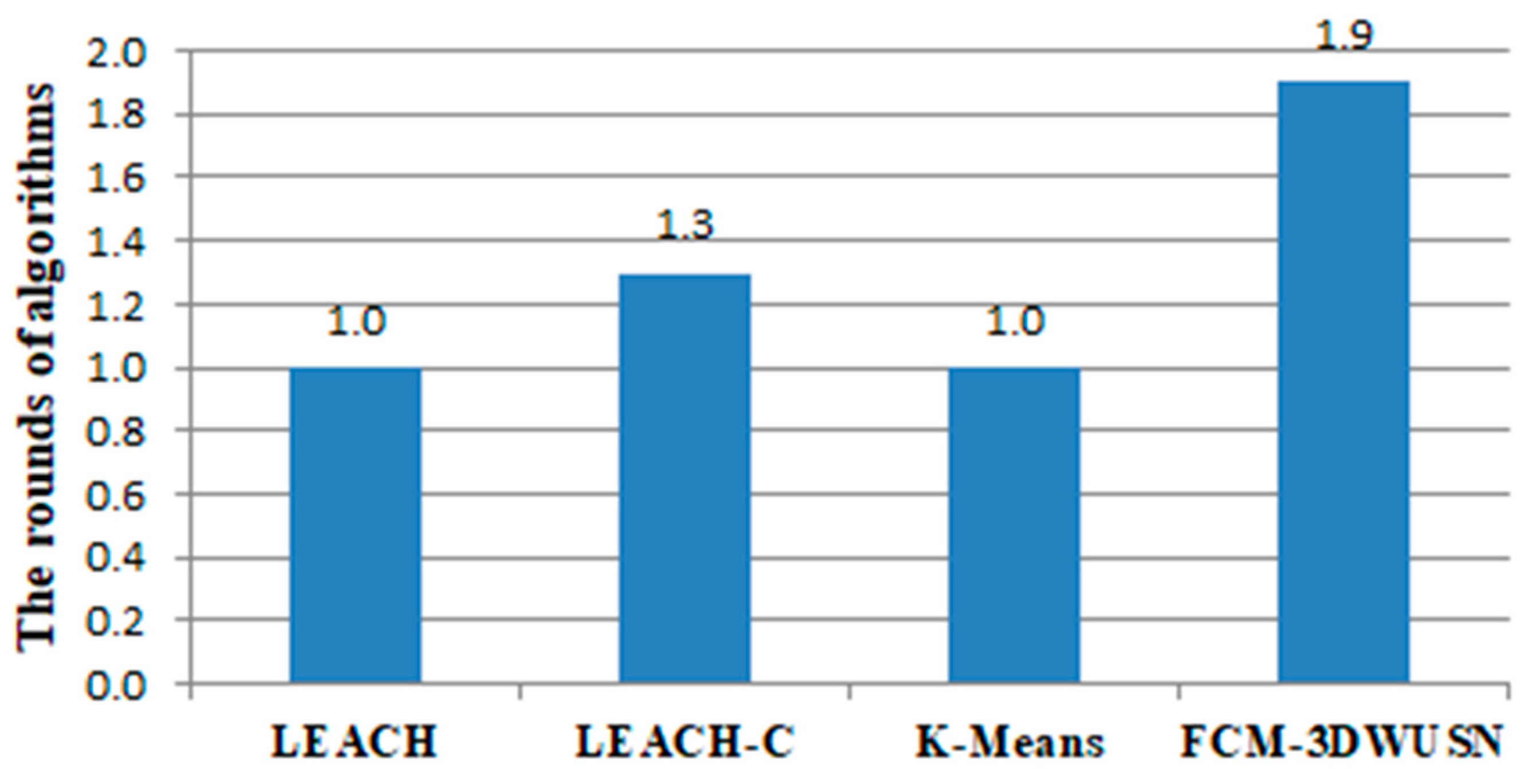

Table 1.
Parameters of the model.
| Parameter | Value |
|---|---|
| Initial node power | 5J |
| N | 1000 |
| 250 m | |
| 50 nJ/bit | |
| 5 pJ/bit | |
| εmp | 0.0013 pJ/bit/m4 |
| εfs | 10 pJ/bit/m2 |
| L | te |
Table 2.
The power efficiency of the models on different terrain.
| Terrain | LEACH | LEACH-C | K-Means | FCM-3DWUSN |
|---|---|---|---|---|
| T1 | 182.160 | 293.957 | 138.247 | 174.789 |
| T2 | 195.159 | 155.514 | 129.667 | 162.054 |
| T3 | 208.515 | 514.775 | 154.227 | 169.368 |
| T4 | 164.012 | 384.664 | 116.199 | 119.982 |
| T5 | 209.05 | 240.831 | 187.040 | 179.56 |
| T6 | 173.954 | 517.287 | 144.514 | 102.553 |
| T7 | 212.243 | 189.875 | 167.110 | 116.225 |
| T8 | 240.986 | 451.496 | 175.418 | 112.452 |
| T9 | 191.596 | 234.403 | 134.354 | 98.457 |
| T10 | 152.167 | 435.096 | 92.175 | 114.452 |
Disclaimer/Publisher’s Note: The statements, opinions and data contained in all publications are solely those of the individual author(s) and contributor(s) and not of MDPI and/or the editor(s). MDPI and/or the editor(s) disclaim responsibility for any injury to people or property resulting from any ideas, methods, instructions or products referred to in the content. |
© 2024 by the authors. Licensee MDPI, Basel, Switzerland. This article is an open access article distributed under the terms and conditions of the Creative Commons Attribution (CC BY) license (http://creativecommons.org/licenses/by/4.0/).
Copyright: This open access article is published under a Creative Commons CC BY 4.0 license, which permit the free download, distribution, and reuse, provided that the author and preprint are cited in any reuse.


