1. Introduction
With the development of Deep Learning (DL), many supervised methods for HSI classification have achieved extraordinary performance[
1,
2,
3,
4,
5]. However, the traditional supervised methods need manual annotation, which is time-consuming and professional-knowledge-supported, and have a weak capacity to attain cross-domain-invariant representation. It causes a terrible generalization gap between the Source Domain (SD) to the Target Domain (TD). In other words, when encountering cross-scene classification tasks, such as data re-collection by advanced devices, HSIs are affected by sensor nonlinearities, seasonal variations, and weather conditions. These factors result in spectral reflectance variations between SD and TD of the same land cover classes. Despite the same land space and region, the well-pretrained model also fails to achieve exact performance. The naive supervised architecture is presented in
Figure 1.
Domain Generalization (DG) has recently attracted significant attention as a more challenging task setting to tackle this problem. Distincting from Domain Adaption (DA), DG requests to produce generalization models and without any TD samples engaging in training. Currently, most DG works focus on learning visual-level domain-invariant representation from multiple SDs or a single SD [
6,
7,
8].
With the rise of the Contrastive Language-Image Pre-training (CLIP) [
9] model, which is trained on vast (image, text) pairs and achieves a remarkable generalization and zore-shot learning capability. It has become increasingly appealing to adapt a CLIP framework with linguistic information to DG tasks for natural RGB image classification. A question arises: Can we adapt the CLIP domain generalization for cross-scene hyperspectral imagery classification, directly? A markable work [
10] proposed a straightforward multimodal DG framework for HSI, called LDGnet, utilizing the language knowledge to learn visual representation and achieve visual-linguistic alignment. However, due to the substantial disparity between the natural RGB image and the HSI data, the SOTA work, LDGnet, still achieves an inferior performance compared with some traditional DG classification models. This seems a depressing assessment, and the question is why we need to employ the CLIP. There are three potential advantages: Firstly, traditional DG models tackle the domain alignment with domain extension and data augment methods based on variational auto-encoder (VAE) [
11] and generative adversarial networks (GANs) [
12], which special design for single or multiple modalities. As opposed to the traditional methods, fine-tuning is a key step in CLIP, which is demonstrated by [
13,
14], for the diversity of downstream tasks. Once the CLIP’s fine-tuning provides an effective for one modality, it can be easily extended to other modalities, such as multispectral and visible light data. This is the exciting generalization capacity distinguished from the traditional method. Secondly, the language knowledge auxils have been demonstrated to be helpful for multi-modal learning by [
15,
16,
17]. Thirdly, The training time of the CLIP framework has an advantage over traditional discriminative generative (DG) classification tasks due to the preservation of a large portion of pre-trained weights. Based on the above analysis, we have reconsidered the LDGnet. The LDGnet’s architecture is specially designed and can be split into three sections: An Image encoder, a frozen text encoder, and a visual–linguistic alignment strategy. Image encoder extracts the visual features from the image patch and splits it into two branches: one is fed into the classification head for the design of the auxiliary loss and another is fed into the projection layer for the visual–linguistic alignment, where the image encoder is designed by the deep residual 3-D CNN network. the text encoder extracts the linguistic features. Finally, the visual–linguistic alignment strategy can make the semantic space treated as a cross-domain shared space. Fine-grained feature recognition, however, benefits from the contextual information in the background, where this information encapsulates the correlation between each pixel and its neighboring pixels. Yet, the image encoder proposed by LDGnet can not effectively extract long-range contextual information. In addition, this image encoder has a weak ability to extract inter-class correlation, where the inter-class correlation plays a significant role in enhancing across-domain category transferability and classification performance, especially under a sample imbalance situation. Distinct from traditional RGB images, which represent the category information by visual characters, the prior knowledge of land cover classes is mainly reflected by the abundant spectrum of the hyperspectral image so that spatial-spectral features extracted by the image encoder are necessary for classification performance. However, the CLIP has already achieved well-aligned knowledge between image features and linguistic features. In contrast, the joint spatial-spectral features provide additional resistance for feature alignment, due to the large-scale pre-trained CLIP specifically designed for HIS characteristics not yet perfect. In summary, the deficiency exists in the following two stages: 1) In the image feature extraction stage, the image encoder can not attain the inter-class correlation information and global features which harms the category transferability and classification performance, respectively. 2) In the visual-linguistic alignment stage, the spatial-spectral features and linguistic features can not be simply and directly aligned without the already well-aligned knowledge from pre-trained CLIP on the HSI data.
In this paper, for the former, we propose a novel image encoder, which equips a simple encoder-only transformer [
18] that can effectively extract the global information and inter-class correlation, instead of the deep residual 3-D CNN network, which tends to fall short in capturing sufficient class correlation information and global spatial-spectral features. For the latter, the key is finding the approach to match the linguistic features and visual features with better alignment, where the visual features contain extra spectral information than traditional images. The processing of alignment in LDGnet has been reconsidered, which made the spatial image features and linguistic features entirely isolated during encoding and there is no bridge for inter-model information flow before the final matching, where inter-modality information means the interactions between visual features and linguistic features. It will work because generic visual and text representations have been obtained by CLIP, which is pre-trained by large-scale image-text pairs, so they can directly align via cosine similarities calculation, but this convenience can not be promoted to alignment between spatial-spectral features and linguistic features. According to this problem, A mechanism of the interaction between two modalities, which is composed of a special cross-attention, has been proposed. With this mechanism, the category information, which is derived from the spatial-spectral features, can make the text semantics become visual-aware and image-conditional, instead of remaining the same for the entire dataset. Correspondingly, the linguistic features make the more distinctive spatial-spectral features, which from more informative spatial regions and more instrumental bands of spectrums, be focused on. In addition, this cross-attention mechanism provides a moderate parameter that can play a role as an adapter to achieve efficient freshly learned knowledge learning via fine-tuning.
In particular, both two improved modules, the image encoder and cross-attention mechanism, have been designed as simply and effectively as possible to avoid conducting extra learnable parameters in supposed to tackle over-fitting caused by insufficient training data of the HSI dataset. The construction of the image encoder can be simply described as follows: a 3-D convolution layer, a specially designed DW convolution [
19] layer, and a transformer encoder with single-head attention mechanism, which omits cls token. In addition, the cross-attention module for the Inter-Modality, which is abbreviated as Linguistic-Interact-with-Visual Engager (LIVE) for full text, only is implemented by several linear layers to generate queries, keys, and values in both the visual branch and the text branch. Extensive experiments demonstrate the superiority of our method.
In summary, our main contributions are as follows:
We design a special image encoder in the visual branch of the CLIP for HSI data characteristics, where this encoder can extract the spatial-spectral features with global-ranged and category correlation.
The LIVE module was proposed to improve the interaction between two modalities before the final matching. With this module, visual features will become more distinctive, and correspondingly linguistic features will be visual-features-based adaptive, instead of being invariable.
Extensive experiments demonstrate the proposed method has a better performance compared with the SOTA work with a CLIP framework for HSI domain Generalization.
2. Materials and methods
2.1. Related Work
2.1.1. Domain Generalization (DG)
DG presents a more formidable challenge than DA, as it seeks to learn the model exclusively through SD data during the training phase without requiring access to TD. The model’s extension to TD occurs in the zero-shot inference stage. Current DG methodologies are broadly classified into two categories: multi-source DG and single-source DG. Various methods explicitly address domain shift among multiple SD domain representations by minimizing differences in feature distributions, employing techniques such as MMD [
20], second-order correlation [
21], and Wasserstein distance [
22]. For the single-source DG, the prevalent approach involves extensive data augmentation. These methods typically amplify or generate out-of-domain samples related to SD, subsequently incorporating these samples into model training to facilitate the transition from SD to TD. The overarching objective of data generation is to produce diverse and plentiful data to enhance generalization. Notably, techniques like variational auto-encoder (VAE) [
11] and generative adversarial networks (GANs) [
12] are frequently harnessed for this purpose.
2.1.2. CLIP
CLIP (Contrastive Language-Image Pre-training), introduced by [
9], stands as a groundbreaking advancement in vision-language learning, demonstrating considerable potential in acquiring generic visual representations through contrastive pre-training. Leveraging its impressive transferability, the effective adaptation of CLIP to downstream tasks has been extensively explored, such as Context Optimization (CoOp), proposed by [
23], introduces learnable prompts for textual inputs as opposed to handcrafted ones, drawing inspiration from prompt learning [
24]. Adopting a strategy reminiscent of adapters [
25], CLIP-Adapter [
14] integrates a lightweight adapter module to generate adapted multi-modal features. Meanwhile, Tip-Adapter [
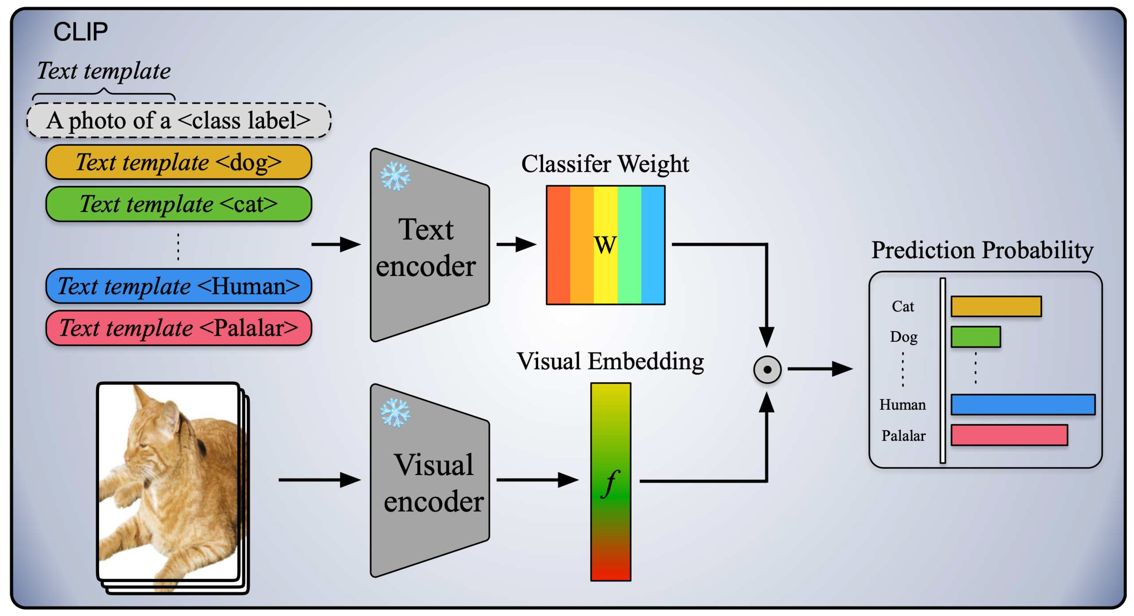
26] substantially reduces training costs by implementing a key-value cache model. The pipeline of naive CLIP is shown in
Figure 2.
2.1.3. Prompt Engineering
Inspired by the success of GPT-3, CLIP embarks on training a substantial contrastive learning model using a vast dataset comprising over 400 million image-text pairs. Notably, CLIP showcases the capability for prompt-based zero-shot visual classification. Serving as the foundation, subsequent advancements such as CoOp (Context Optimization) by [
27]. and CPT (Continuous Prompt Tuning) by [
28] extend these capabilities. These studies demonstrate that optimizing continuous prompts can significantly outperform manually designed discrete prompts in various vision tasks. In this paper, an HSI of {class name} is used as a template to construct coarse-grained text descriptions in a cloze way, which is proposed by [
10]. Analogously, fine-grained text is described manually combined the prior knowledge.
2.2. Proposed Method
In this section, we first introduce the overall network, and then we present the details of the proposed model, including the image encoder and LIVE module. finally, we provide some variants of the proposed model.
2.2.1. Overall Network
Assume that
and
is the data and labels from SD, respectively, where
N denotes the number of source samples and
d denote the channels of HSI data cube. Correspondingly,
is reprensed as the data from TD. We do the same prompt engineering as [
10] introduced. The text is made up of one coarse-grained prompt and two fine-grained prompts corresponding to each sample. The
and
denote the image (visual) encoder and text encoder, respectively. The HSI patches and text are respectively fed into the
and
, to extract the spatial-spectral features (visual features
) and linguistic features (text features
).
is a language-model transformer[33][34] (in LDGnet) and details of the
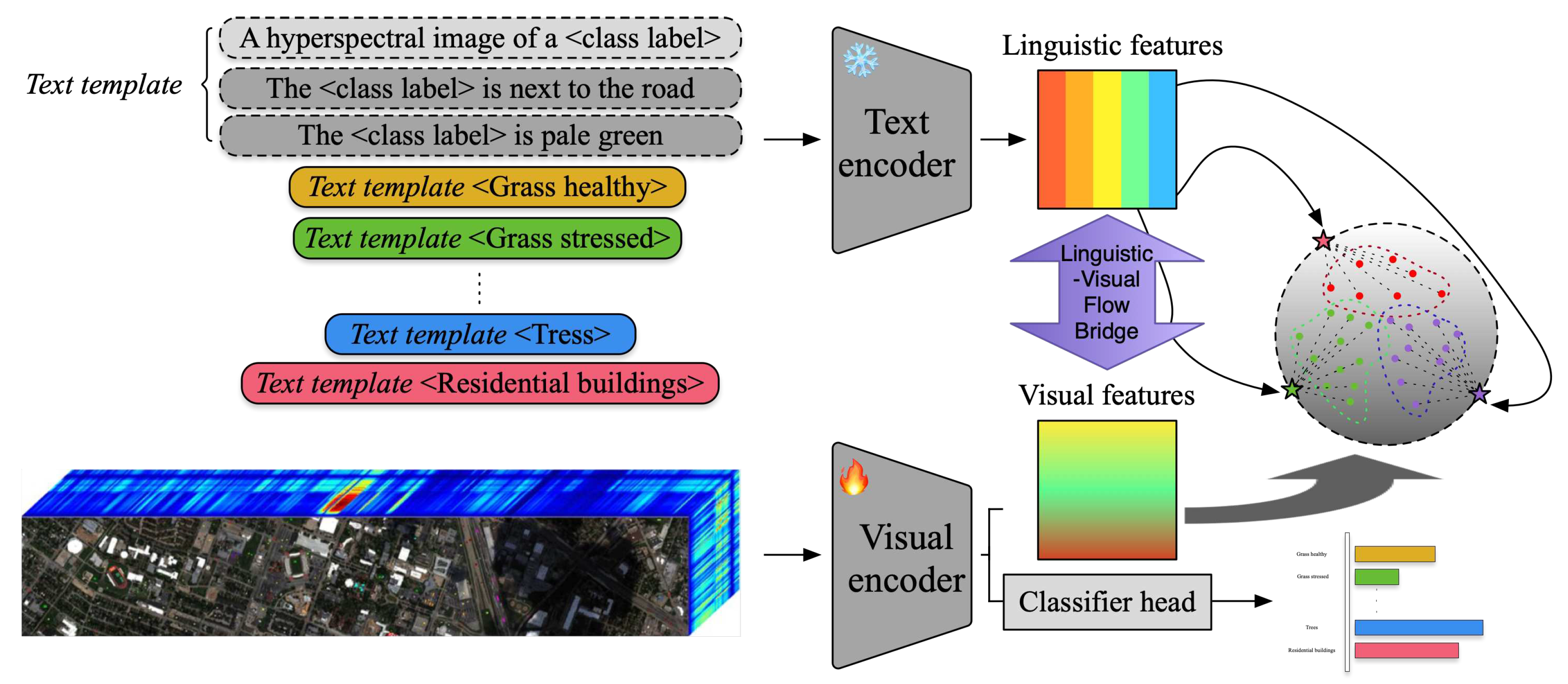
will be elaborated in the subsection. Then the spatial-spectral features are delivered to the projection head (Proj) and the classification head (Cls), simulately. The Proj can project the visual features for interacting with linguistic features and visual-linguistic alignment. The Cls is used to implement assistant loss by calculating the cross-entropy. The pipeline of our proposed architecture is shown in
Figure 3.
2.3. Image Encoder
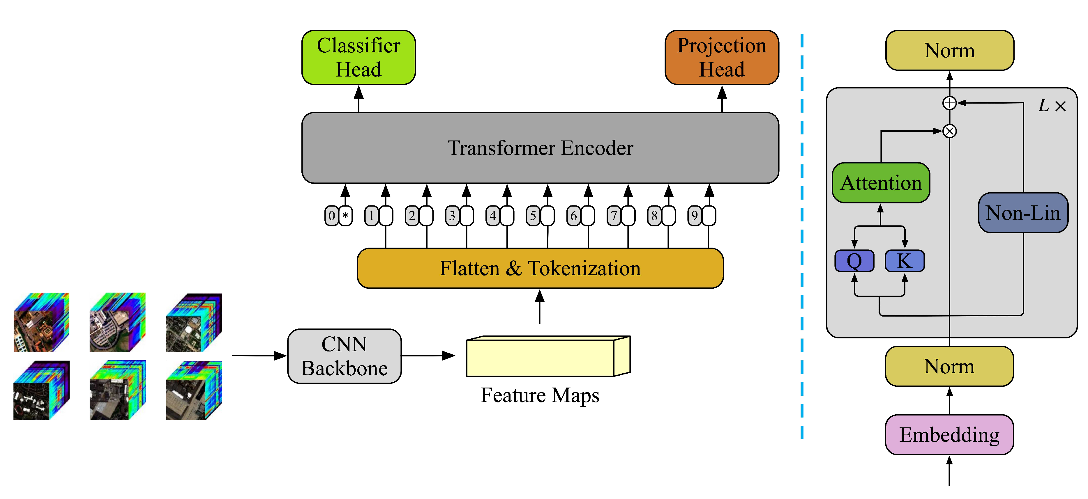
The image encoder consists of a CNN backbone and a simple transformer encoder, as shown in
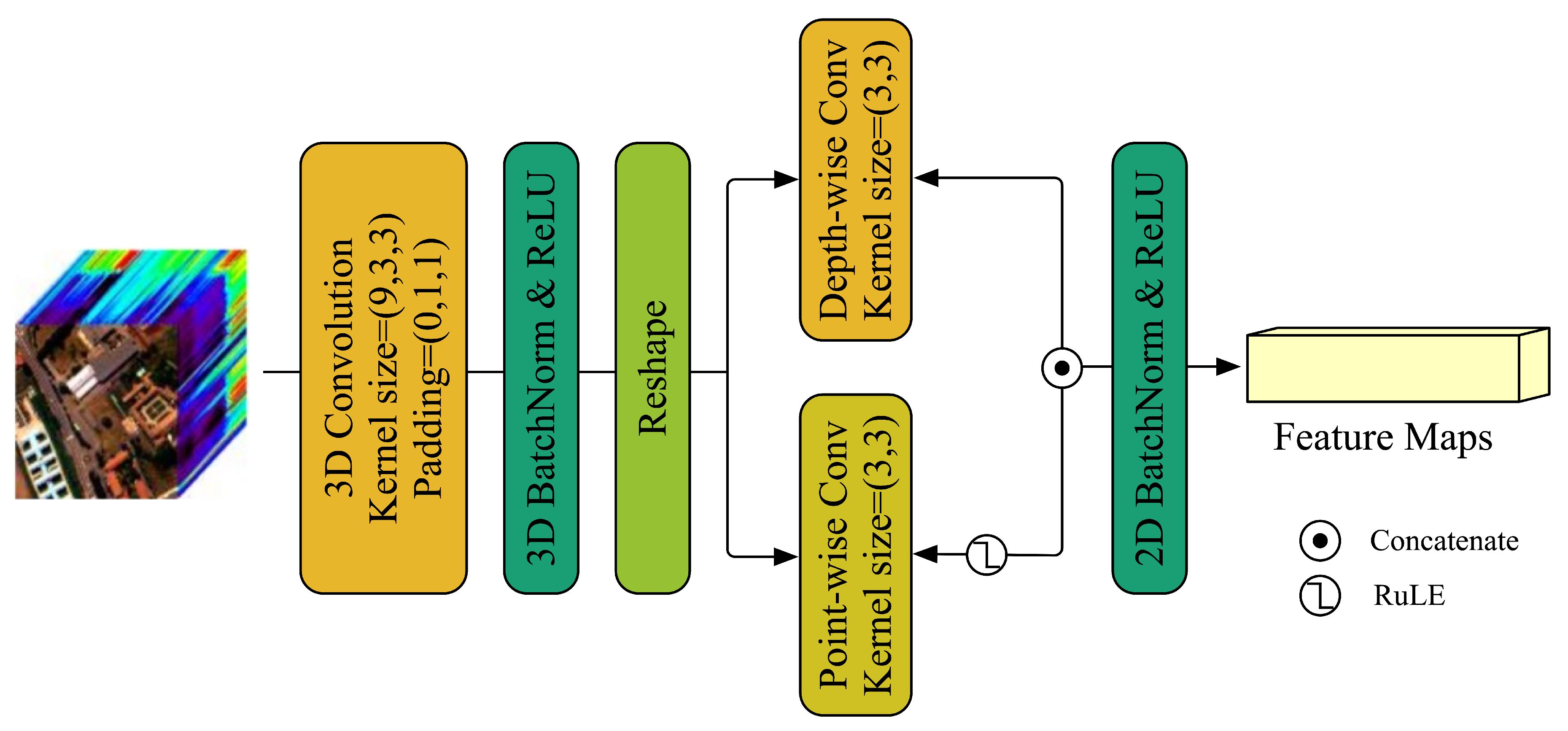
Figure 4 and the detail of the CNN backbone can be described in
Figure 5. The subcubes
of
from SD are delivered to the CNN backbone for extracting the spatial-spectral features and reducing its spectral dimensions, then the feature embedding is used by the transformer to extract more distinctive features with contextual feature and inter-class correlation.
The proposed CNN backbone consists of 3D-CNN with kernel size to extract the local features and spatial-spectral features, then the padding is used to keep the spatial dimensions the same and reduce the spectral dimensions for lightweight. Correspondingly, a DW block is designed by a bi-branch framework. The depth-wise convolution with kernel size is adopted in one of the branches and a ReLU activation function also is introduced. Correspondingly, the point-wise convolution with kernel size of is equipped in the other. Further, The ultimate feature maps are produced by multiplying the outputs of two branches and adding the output of 3D-CNN utilizing the residual connection. Finally, the feature maps are fed into a simple transformer encoder to extract the inter-class correlation and global contextual features, then the transformer outputs the and Cls matrix. Here, the L is the number of transformer encoder blocks and is initialized with 3 for obtaining a more shallow transformer. In this case, the residual connection is not only unnecessary, because the outputs are low-level inlinear and identity-like, but increases redundancy and latency. To tackle this problem, we introduce a skipless module, which is composed of dual-branch attention without value.
2.4. LIVE Module
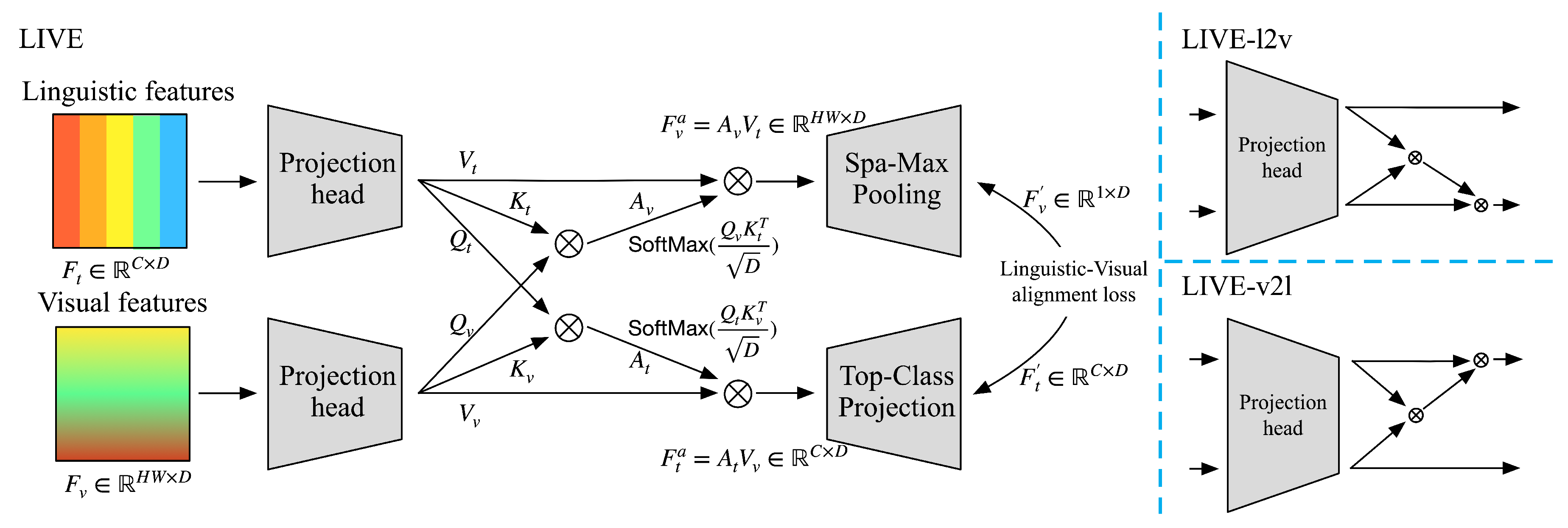
As shown in
Figure 6,
and
respectively denote the linguistic features and visual features, which outputted by the corresponding encoder. Here,
C denotes the Classes number, and
D denotes the feature Dimension. We propose projection layers to produce individual queries, keys, and values. Specifically,
,
, and
are produced by the projection head using the linguistic features as input. Correspondingly,
,
, and
denote value, key, and query projected from visual features.
Where
denotes the projection head, which consists of a linear layer of
dimension, and the outputs are split equally as
Q,
K,
V on D dimension. Then two attention maps can be calculated, which are denoted as
and
.
where
and
are respectively for linguistic and visual features update.
where and respectively denote that updated visual and textual features. With this cross-attention mechanism, the information communication and interaction bridge has been built between linguistic modality to visual modality to align the spatial-spectral and linguistic features with more reasonable and available. On the one hand, the high-level abstract visual features will be focused on with text guidance. On the other hand, this bridge makes the linguistic features flexible, image-conditional, and self-adapted instead of fixed.
In the ultimate stage, We proposed the top-class projection module to extract the linguistic feature vectors corresponding to the class with the highest probability for each sample in the text data. Subsequently, these selected feature vectors are projected into a new semantic space in preparation for domain alignment. Spa-Max Pooling is adopted to retain the distinguish characters and reduce its spatial dimension.
2.5. Loss Function
Our loss function is composed of the classification loss and the linguistic-visual alignment loss [
29]. Firstly, the classification loss can be denoted as
where the
is Cross-Entropy loss function and
is the output of classification branch of our model. In addition, the linguistic-visual alignment loss (
) is inspired by supervised contrastive learning [36](in LDGnet), which is defined as
where the and denote the visual feature and textual feature, respectively in minibatch, and means the positive and negative samples of visual feature. Correspondingly, and also are the positive and negative samples of two modalities features. Notably, this loss exists for both coarse-grained and fine-grained text prompts, denoted as and .
Integrating the above loss functions, the total loss is represented as
where the and is hyperparameters for balancing the and control the contribution of both and , respectively.
2.6. Variantes of Proposed Module
For the LIVE module, three versions can be selected,
ALL-LIVE denotes that the module is used for aligning both coarse-grained text and fine-grained with visual features,
Coarse-LIVE denotes that only is available in alignment between coarse-grained text and visual features, and similarly the
Fine-LIVE is designed for only fine-grained text and visual features alignment. For each version, we explore and compare the performance of the unidirectional or bidirectional bridge that has been used for information interaction. For all descriptions and experiments, the bidirectional Coarse-LIVE module is the default, and more detailed discussions will be provided in
Section 3.3.4.
Figure 1.
The pipeline of the traditional supervised method for image classification.
Figure 1.
The pipeline of the traditional supervised method for image classification.
Figure 2.
The pipeline of the CLIP for image classification.
Figure 2.
The pipeline of the CLIP for image classification.
Figure 3.
Pipeline of the proposed architecture. Firstly, the frozen text encoder and the visual encoder extract the linguistic and visual features, respectively. Then, the LIVE module makes the two modalities mutually communicate to achieve better alignment. Meanwhile, the visual features are fed into the classifier head to obtain the prediction probability.
Figure 4.
The structure of the image encoder. The Non-Lin denotes a non-linear layer for embedding feature projection.
Figure 4.
The structure of the image encoder. The Non-Lin denotes a non-linear layer for embedding feature projection.
Figure 5.
The framework of the CNN backbone.
Figure 5.
The framework of the CNN backbone.
Figure 6.
The architecture of the proposed LIVE module is depicted on the left side of the image, while on the right side are its two variants based on bidirectional or unidirectional cross-attention mechanisms, where the l2v and the v2l mean the text-guided visual and linguistic features alignment and image-conditional linguistic and visual features alignment framework, respectively.
Figure 7.
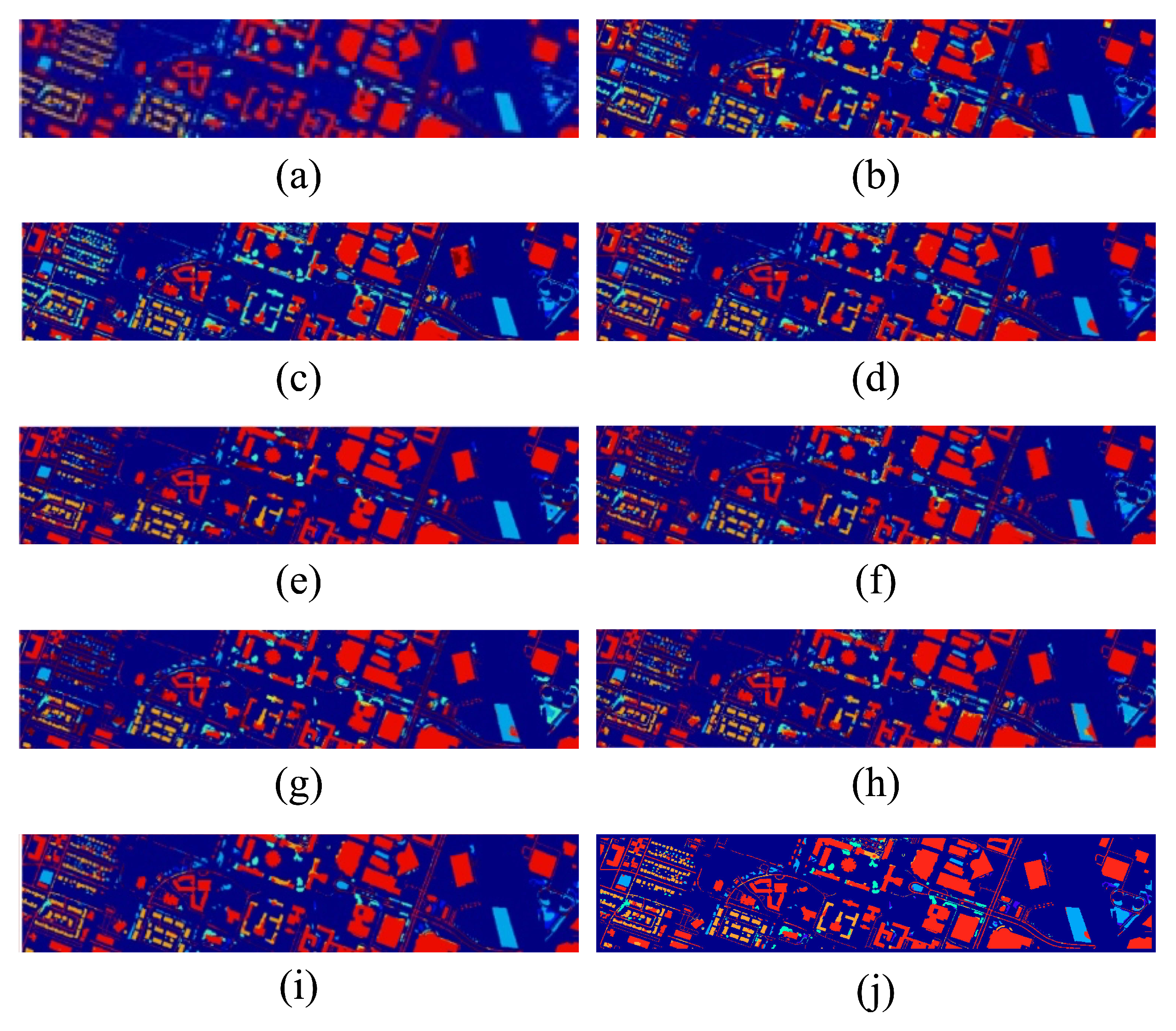
The classification maps of the different methods on the Houston 18 dataset. (a) Ground truth. (b) DAAN. (c) MRAN. (d) DSAN. (e) HTCNN. (f) PDEN. (g) LDSDG. (h) SagNet. (i) LDGnet. (j) LIVEnet.
Figure 7.
The classification maps of the different methods on the Houston 18 dataset. (a) Ground truth. (b) DAAN. (c) MRAN. (d) DSAN. (e) HTCNN. (f) PDEN. (g) LDSDG. (h) SagNet. (i) LDGnet. (j) LIVEnet.
Figure 8.
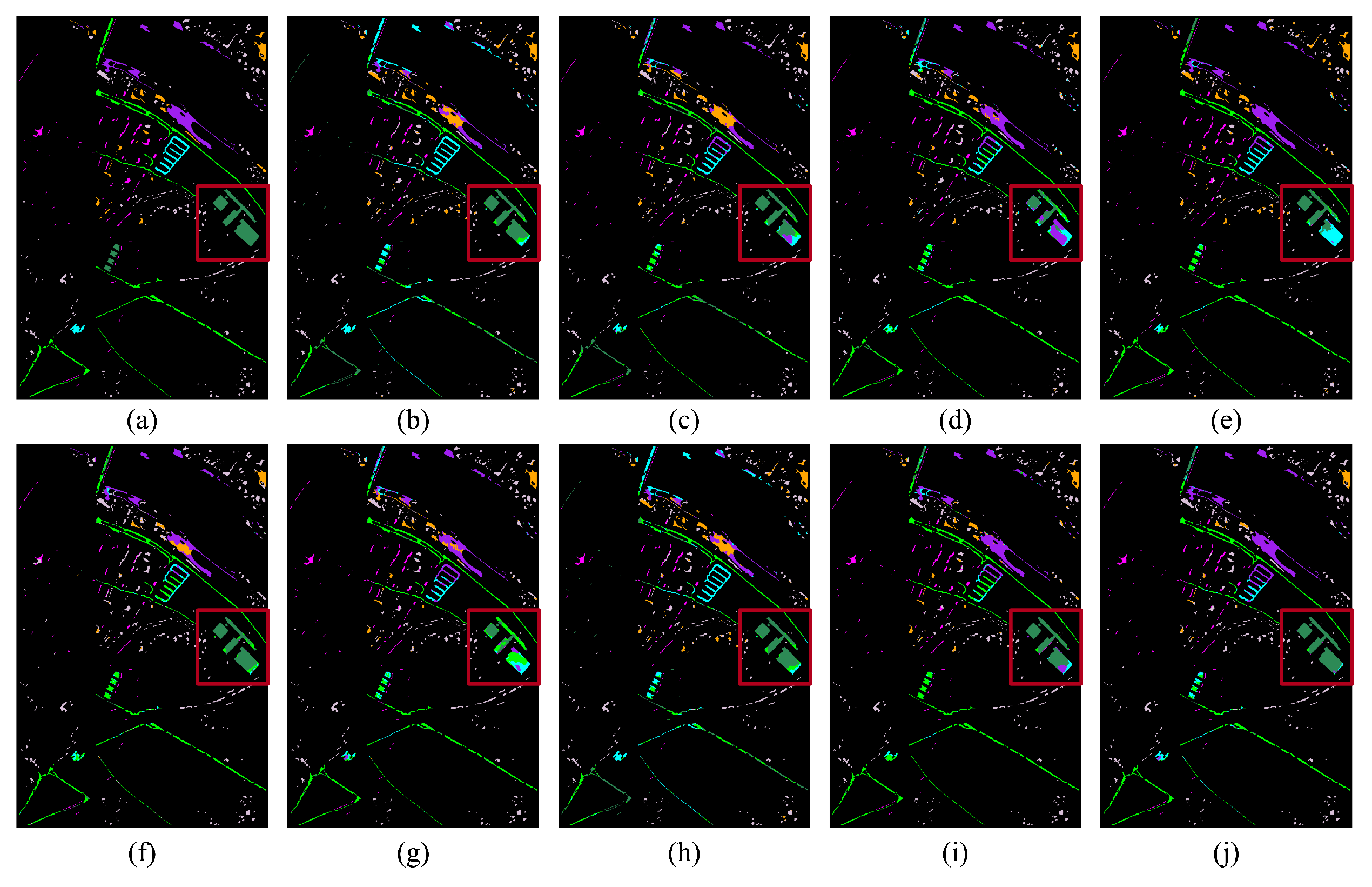
The classification maps of the different methods on the PC dataset. (a) Ground truth. (b) DAAN. (c) MRAN. (d) DSAN. (e) HTCNN. (f) PDEN. (g) LDSDG. (h) SagNet. (i) LDGnet. (j) LIVEnet.
Figure 8.
The classification maps of the different methods on the PC dataset. (a) Ground truth. (b) DAAN. (c) MRAN. (d) DSAN. (e) HTCNN. (f) PDEN. (g) LDSDG. (h) SagNet. (i) LDGnet. (j) LIVEnet.
Figure 9.
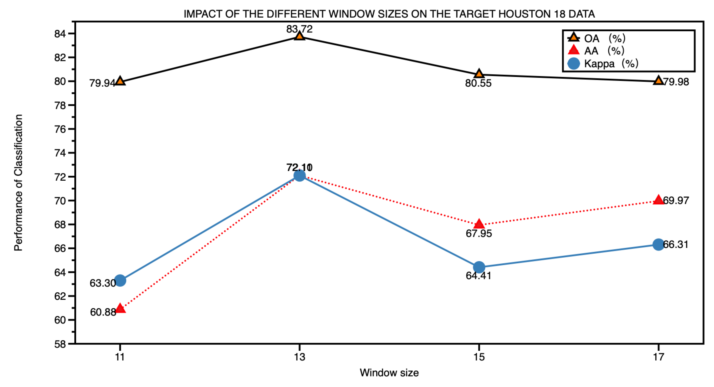
The impact of the different window sizes for classification on target Houston 18 data.
Figure 9.
The impact of the different window sizes for classification on target Houston 18 data.
Table 1.
Land-cover classes and the number of samples of the Houston13 and Houston18 datasets
Table 1.
Land-cover classes and the number of samples of the Houston13 and Houston18 datasets
| Class No. |
Land-cover Class |
Number of Samples (Houston 13) |
Number of Samples (Houston 18) |
| 1 |
Stressed Grass |
345 |
1353 |
| 2 |
Grass stressed |
365 |
4888 |
| 3 |
Trees |
365 |
2766 |
| 4 |
Water |
285 |
22 |
| 5 |
Residential buildings |
319 |
5347 |
| 6 |
Non-residential buildings |
408 |
32459 |
| 7 |
Road |
443 |
6365 |
| |
Total |
2530 |
53200 |
Table 2.
Land-cover classes and the number of samples of the UP and PC
Table 2.
Land-cover classes and the number of samples of the UP and PC
| Class No. |
Land-cover Class |
Number of Samples (UP) |
Number of Samples (PC) |
| 1 |
Tree |
3064 |
7598 |
| 2 |
Asphalt |
6631 |
9248 |
| 3 |
Brick |
3682 |
2685 |
| 4 |
Bitumen |
1330 |
7287 |
| 5 |
Shadow |
947 |
2863 |
| 6 |
Meadow |
18649 |
3090 |
| 7 |
Bare soil |
5029 |
6584 |
| |
Total |
39332 |
39355 |
Table 3.
CLASSIFICATION ACCURACY (%) OF DIFFERENT METHODS FOR THE TARGET HOUSTON 18 DATA
Table 3.
CLASSIFICATION ACCURACY (%) OF DIFFERENT METHODS FOR THE TARGET HOUSTON 18 DATA
| Class No. |
DAAN |
MRAN |
DSAN |
HTCNN |
PDEN |
LDSDG |
SagNet |
LDGnet |
LIVEnet |
| 1 |
68.29 |
41.02 |
62.31 |
11.83 |
46.49 |
10.13 |
25.79 |
61.71 |
44.42 |
| 2 |
77.80 |
76.94 |
77.50 |
70.11 |
77.60 |
62.97 |
62.79 |
77.45 |
77.41 |
| 3 |
67.50 |
65.91 |
74.55 |
54.99 |
59.73 |
60.81 |
48.66 |
62.08 |
62.33 |
| 4 |
100.0 |
100.0 |
100.0 |
54.55 |
100.0 |
81.82 |
81.82 |
95.45 |
81.82 |
| 5 |
47.69 |
36.90 |
73.39 |
55.60 |
49.62 |
45.65 |
59.57 |
69.53 |
84.65 |
| 6 |
79.49 |
82.68 |
86.84 |
92.85 |
84.98 |
89.22 |
89.28 |
91.57 |
92.03 |
| 7 |
45.12 |
56.43 |
46.33 |
46.47 |
64.21 |
44.15 |
34.99 |
45.42 |
60.25 |
| OA |
70.45±1.54 |
72.11±1.79 |
78.21±1.05 |
77.67±2.11 |
75.40±1.76 |
74.23±1.49 |
73.01±1.81 |
80.34±1.74 |
83.39±1.47 |
|
() |
53.86±2.14 |
55.03±2.86 |
64.10±1.83 |
60.18±3.07 |
55.87±2.92 |
55.42±2.27 |
55.29±3.50 |
65.80±2.59 |
71.83±2.89 |
Table 4.
CLASSIFICATION ACCURACY (%) OF DIFFERENT METHODS FOR THE TARGET PC DATA
Table 4.
CLASSIFICATION ACCURACY (%) OF DIFFERENT METHODS FOR THE TARGET PC DATA
| Class No. |
DAAN |
MRAN |
DSAN |
HTCNN |
PDEN |
LDSDG |
SagNet |
LDGnet |
LIVEnet |
| 1 |
71.98 |
59.16 |
93.93 |
96.06 |
85.93 |
91.09 |
98.35 |
95.20 |
99.55 |
| 2 |
78.98 |
85.15 |
79.80 |
57.70 |
88.56 |
73.51 |
59.76 |
82.79 |
84.95 |
| 3 |
19.37 |
46.18 |
53.97 |
2.76 |
61.34 |
2.23 |
5.40 |
80.48 |
47.97 |
| 4 |
58.67 |
69.58 |
75.75 |
93.25 |
85.49 |
71.72 |
87.03 |
85.11 |
84.28 |
| 5 |
70.87 |
64.58 |
99.44 |
89.94 |
87.95 |
71.04 |
93.19 |
93.15 |
81.28 |
| 6 |
83.07 |
89.22 |
74.43 |
70.97 |
79.26 |
57.12 |
49.81 |
66.93 |
45.08 |
| 7 |
55.59 |
60.10 |
67.31 |
42.28 |
64.75 |
78.13 |
57.94 |
81.97 |
98.51 |
| OA |
66.71±2.15 |
69.01±1.21 |
78.21±1.10 |
68.31±1.62 |
80.27±1.38 |
70.88±1.55 |
69.28±1.11 |
82.53±1.24 |
83.94±0.99 |
|
() |
59.76±3.47 |
63.04±1.90 |
74.10±1.57 |
62.17±2.57 |
76.81±1.92 |
64.06±2.07 |
63.04±1.67 |
78.85±1.78 |
80.51±1.52 |
Table 5.
EXECUTION TIME OF ONE EPOCH TRAINING IN COMPARISON METHODS ON THE UH AND PAVIA DATASET
Table 5.
EXECUTION TIME OF ONE EPOCH TRAINING IN COMPARISON METHODS ON THE UH AND PAVIA DATASET
| Datasets |
DAAN |
MRAN |
DSAN |
HTCNN |
PDEN |
LDSDG |
SagNet |
LDGnet |
LIVEnet |
| Houston 2013 |
16.04 |
14.01 |
15.94 |
32.22 |
4.79 |
40.28 |
7.63 |
18.19 |
15.61 |
| UP |
27.97 |
28.33 |
29.02 |
47.99 |
13.05 |
65.93 |
19.76 |
68.02 |
62.50 |
Table 6.
CLASSIFICATION ACCURACY (%) OF DIFFERENT SERVICE OBJECT VARIANTS FOR THE TARGET HOUSTON 18 DATA
Table 6.
CLASSIFICATION ACCURACY (%) OF DIFFERENT SERVICE OBJECT VARIANTS FOR THE TARGET HOUSTON 18 DATA
| Class No. |
All-LIVE |
Fine-LIVE |
Coarse-LIVE |
| 1 |
41.24 |
47.89 |
44.23 |
| 2 |
69.46 |
71.62 |
77.59 |
| 3 |
60.88 |
59.58 |
62.57 |
| 4 |
81.82 |
100.0 |
81.89 |
| 5 |
83.60 |
76.30 |
84.38 |
| 6 |
92.05 |
92.58 |
92.89 |
| 7 |
58.24 |
56.62 |
61.11 |
| OA |
82.17 |
81.87 |
83.72 |
| AA |
69.61 |
72.09 |
72.11 |
|
() |
69.22 |
68.11 |
72.10 |
Table 7.
CLASSIFICATION ACCURACY (%) OF DIFFERENT FRAMEWORKS OF COARSE-LIVE MODULE FOR THE TARGET HOUSTON 18 DATA
Table 7.
CLASSIFICATION ACCURACY (%) OF DIFFERENT FRAMEWORKS OF COARSE-LIVE MODULE FOR THE TARGET HOUSTON 18 DATA
| Class No. |
LIVE-l2v |
LIVE-v2l |
LIVE |
| 1 |
15.23 |
60.90 |
44.23 |
| 2 |
80.16 |
65.22 |
77.59 |
| 3 |
62.62 |
60.30 |
62.57 |
| 4 |
81.82 |
81.82 |
81.89 |
| 5 |
75.56 |
87.94 |
84.38 |
| 6 |
92.64 |
89.98 |
92.89 |
| 7 |
61.60 |
63.33 |
61.11 |
| OA |
82.53 |
82.03 |
83.72 |
| AA |
67.09 |
72.78 |
72.11 |
|
() |
69.86 |
69.99 |
72.10 |
Table 8.
IMPACT OF THE DIFFERENT WINDOW SIZES ON THE TARGET HOUSTON 18 DATA
Table 8.
IMPACT OF THE DIFFERENT WINDOW SIZES ON THE TARGET HOUSTON 18 DATA
| Window size |
OA |
AA |
Kappa (%) |
Execution time (s) |
Training parameters (M) |
| 11 |
79.94 |
60.88 |
63.30 |
15.16 |
2.08 |
| 13 |
83.72 |
72.11 |
72.10 |
15.61 |
2.97 |
| 15 |
80.55 |
67.95 |
64.41 |
19.09 |
3.73 |
| 17 |
79.98 |
69.97 |
66.31 |
21.29 |
4.75 |
Table 9.
Ablation experiment on the UH dataset
Table 9.
Ablation experiment on the UH dataset
| Cases |
OA (%) |
Kappa (%) |
| baseline |
79.13 |
77.62 |
| w/o image encoder |
81.20 |
69.53 |
| w/o LIVE |
79.42 |
78.10 |
| LIVEnet |
83.39 |
71.83 |

