1. Introduction
1.1. Background and Motivation
Recently, Phasor Measurement Units (PMU) have been widely adopted by many power system operators for monitoring their systems. The PMU measurements are gathered at a high sampling speed between 30 and 240 samples per second [
1,
2]. In addition to the bus voltage magnitude, phase-angle data can also be obtained from PMU measurements [
2]. The installation of PMU units is globally popular for new substations to utilize this data [
3]. For example, PMU data can be used for real-time frequency-stability monitoring, state estimation, disturbance analysis, and wide-area control. Considering the installation of large-scale renewable energy sources with high output fluctuations, the importance of real-time power system monitoring and rapid analysis by PMU units should be emphasized.
One of the interesting fields is the effort to apply these PMU measurements to artificial intelligence (AI) models. Many studies have focused on developing models that predict the power system stability using AI techniques. For instance, local frequency measurements using PMU devices are gathered and used to train an AI model that predicts the global short-term system frequency. In addition, phase angle measurements from different buses can be applied to rotor-angle stability prediction models.
Most previous studies have focused only on increasing the accuracy of these prediction models. In general, it is required for the prediction models to have complicated architectures with large hyperparameters to obtain good accuracies. This inevitably results in significant calculation burden and increased memory resources during the training stage. In this context, the application of these AI skills is limited to computers with very high performance.
Unlike the aforementioned approaches, training improvement methods are proposed in this article to relieve the huge computational burden during the training stage. The aim is to extend AI applications with reduced training difficulty and an acceptable output performance.
1.2. Literature Review
The majority of previous studies on AI prediction models have focused on improving prediction outputs. These outputs are evaluated based on either classification accuracy or regression error. Large-scale training, validation, and testing data are required to train and assess the models. The prediction accuracy improvement of the transient stability assessment in the IEEE 39-bus system models is examined in [
4]. Based on long short-term memory (LSTM) and support vector machine (SVM) methods, a fault detection model after a transmission line trip is developed in [
5]. The transient rotor-angle behaviors of power system models can be trained using physics-informed neural networks (PINN) [
6,
7]. Predictions of power system frequency dynamics by PINN are studied in [
8,
9,
10].
The implementation of AI techniques is also popular for time-series data prediction in the field of power system engineering. The hourly output predictions of renewable energy sources, such as photovoltaics and wind power plants, are discussed in [
11,
12,
13,
14,
15]. The effectiveness of the LSTM model for short-term industrial load demand forecasting is validated in [
16]. The prediction of time-series frequency data in the US for one second is formulated by a state space model in [
17]. A prediction model of the frequency trajectory for three minutes is proposed in [
18] using a Bayesian network. An artificial neural network (ANN) model is adopted to train the time-series frequency trajectory on an hourly time-scale [
19]. The utilization of auto-regressive moving average (ARMA) models for the prediction are also analyzed in [
20,
21]. Under-frequency load shedding by a wide-area-monitoring-system (WAMS)-based short-term frequency trajectory prediction is explained in [
22].
Moreover, proposals for AI-based time-series trajectory predictions have been examined in other research fields. The predictions of the motion trajectories of a vehicle and vessel are assessed in [
23,
24], respectively. Aircraft route trajectory prediction is discussed using hybrid neural network models in [
25,
26]. Pedestrian path predictions based on bidirectional LSTM networks with automatic trajectory clustering are proposed in [
27,
28]. A trajectory prediction model for autonomous air combat vehicles is investigated in [
29].
These studies have attempted to increase the accuracy of prediction outputs with well-designed or optimized hyperparameters of the training models. In contrast, few studies have focused on the efficiency of the training process with constrained training hyperparameters. No trial to reduce the calculation burden during the training stage has been conducted.
1.3. Contribution in This Paper
The objective of this paper is to improve the training process of the ANN trajectory prediction models. First, the original trajectory of the training data is split into several different segments based on the minimum, maximum, and inflection points. Consequently, the original training problem can be divided into sub-problems. This reduces the complexity of each training problem. In addition, the time-derivative terms of the training data and ANN output trajectories are added to the loss function. Inspired by physics-informed neural networks, ANN models can be trained with fewer calculation resources by using this augmented loss function.
The main contribution of this paper is explained as follows:
1) The effectiveness of the training improvements is analyzed in constrained training conditions. This aims to reduce the training calculation difficulty of the ANN models. The output performance of the ANN models may not be optimal, but is still reasonable.
2) The ANN trajectory output is a closed analytic form and differentiable [
30], and has better applicability than discrete PMU data. Furthermore, the required number of parameters for the time-series data calculation is much less than that in conventional numerical approaches, such as the Runge-Kutta method [
30].
3) The proposed method can be adopted and extended to other trajectory predictors. In this study, the validity of the training improvements is explained for the rotor-angle and frequency trajectories in power system models. In addition to the applications in the field of power system engineering, the proposed approaches can be used in many other research areas.
These methods have been validated in WSCC three-machine nine-bus and IEEE 39-bus system models. To evaluate the effectiveness of the developed methods, the ANN outputs and original training data are compared to calculate the mean absolute error (MAE) losses after the ANN training process. It has been demonstrated that when ANN training hyperparameters such as the number of neurons, hidden layers, and epochs are constrained, the ANN training results have lower MAE losses and better reflect the original training data compared to the cases without the proposed methods.
This article is organized as follows. An overview of the ANN training improvement techniques is provided in
Section 2. The power system models are explained in
Section 3. The effect of the proposed improvement methods on the ANN model training is presented in
Section 4, and the conclusion is presented in
Section 5.
2. ANN Trajectory Prediction Model
2.1. Concept Overview
The following variables are available from PMU measurements in phasor format: voltage, current, active power, reactive power, frequency, and rate of change of frequency (ROCOF) [
2,
31]. These PMU devices are installed in substations of high-voltage transmission systems. Local PMU measurements are transferred to the control center of the transmission system operator (TSO) using a communication network. The PMU measurement data is sampled in discrete format. The PMU data sampling speed is between 30 and 240 samples per second [
1,
2].
A continuous trajectory predictor can be trained using discrete PMU data. Unlike the original discrete PMU measurements, this continuous trajectory is differentiable and has a closed analytical form [
30]. Thus, it can be said that the applicability of this continuous trajectory is better than that of the PMU data. For example, a TSO can establish several trajectory predictors for representative and frequent system disturbances. This helps the TSO predict the dynamic behaviors of the system and take proper actions to minimize the impact of disturbances.
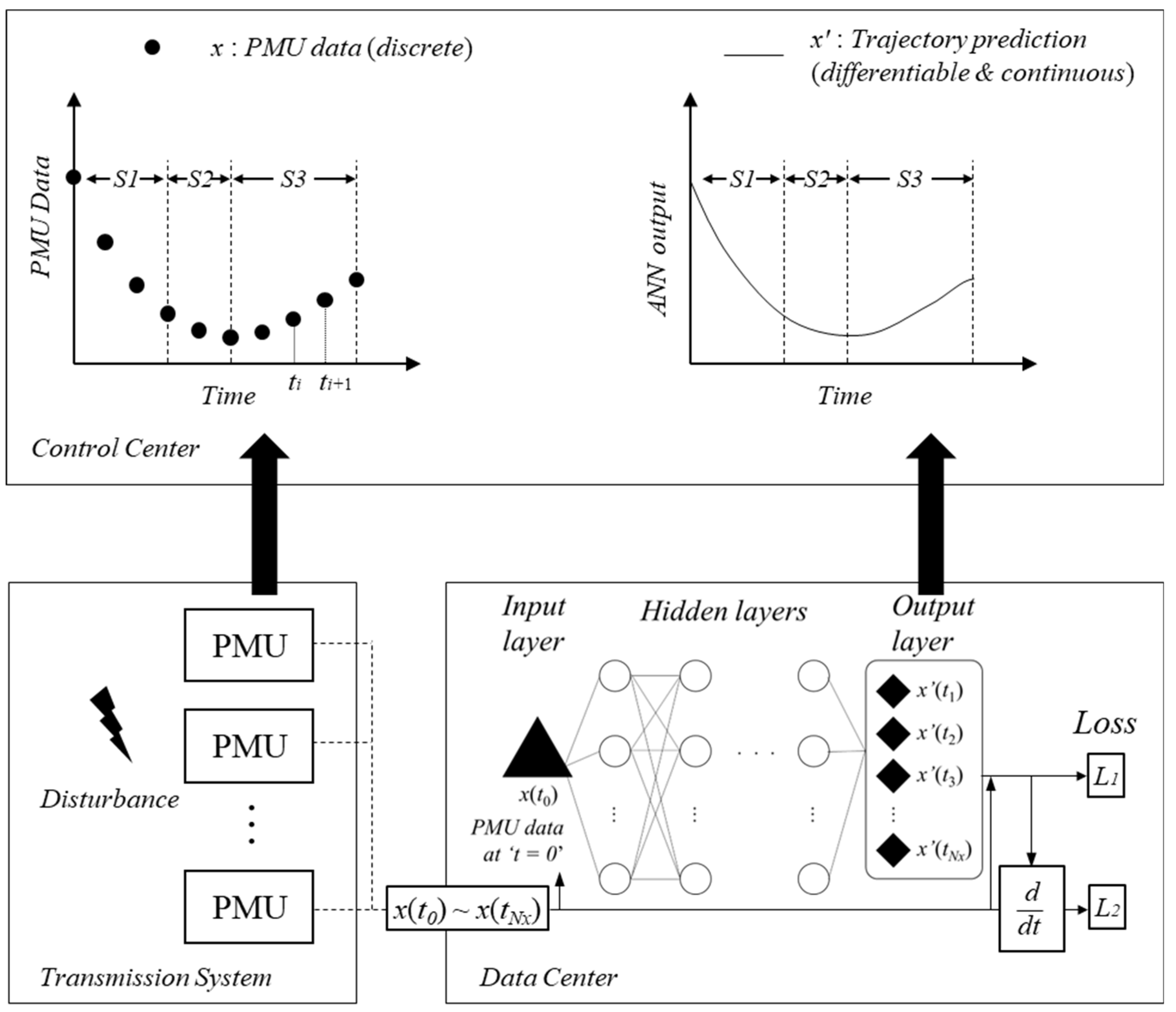
The principle of continuous trajectory prediction using an ANN model is described in
Figure 1. The initial value of the PMU data
x(
t0) is required as the input data for the ANN model. The output data
x’(
t) consist of
Nx time-series data, where
Nx is the total number of output data-sets. If a short time interval between
t =
Ni-1 and Ni is selected, the output data of the ANN model can be handled as a continuous time-series trajectory.
The ANN model training process is summarized as follows. The PMU discrete data x during t = 0 ~ Nx are gathered. Among all the PMU data, the initial value x(t0) is used as the input data of the ANN model. After calculating all hidden layers, the ANN output trajectory x’(t1) ~ x’(tNx) is acquired. The loss function value is evaluated to update the weight and bias parameters of the ANN model based on their gradient values. Therefore, the definition of the loss function directly affects the training stage. The manipulation of a loss function can be considered to improve ANN model training. A detailed explanation of loss function manipulation is provided in the next subsection.
Generally, large-scale big data are used to train and evaluate AI-based prediction models. In addition to the training dataset, validation and testing data are required. On the contrary, this paper aims to improve the training process of ANN models. Hence, we only focus on the training stage of the ANN model. The ANN training results can be evaluated by comparing the PMU training data with the ANN outputs. No validation or testing data are necessary for this process.
2.2. Augmented Loss Function
The loss function of an ANN model is the difference between the target value and ANN output. It is desirable to minimize this loss function value to achieve a good ANN prediction performance. The weight and bias values are adjusted based on the gradients to reduce the loss function. This training process can be handled as an optimization problem which minimizes the loss function by adjusting the weight and bias parameters.
It has been reported that the output prediction accuracy can be increased by incorporating the physical and dynamic characteristics in the loss function. For instance, the swing equation of a power system model is included in the loss function for the identification of state parameters [
32]. An augmented loss function containing the Karush-Kuhn-Tucker (KKT) condition in optimal power flow (OPF) analysis is proposed to reduce the training time and test error [
33].
In this paper, the time-derivative term of the dynamic trajectory is added to improve the ANN model training. Consequently, the weight and bias parameters can be updated by considering not only the training data itself, but also the time-derivative characteristics. The augmented loss function L for the ANN training improvement is defined as follows:
where
L is the total augmented loss function which is composed of two loss terms
L1 and
L2.
L1 is the common mean absolute error (MAE) value. It is calculated as the mean of the absolute values of the error between the ANN trajectory prediction output
x’ and the original training data x in (2). In addition, the time-derivative terms of the ANN prediction output
x’ and training data
x are evaluated in
L2 loss function. This
L2 is obtained by the mean of the absolute values of the error between the time-derivatives of
x’ and
x.
λ is the regularization parameter of
L2 loss function.
2.3. Piecewise Segment Training
In many cases, the transient behavior of time-series trajectories in power systems is nonlinear. It is difficult to train a trajectory predictor model if the trajectory is nonlinear or irregular. To overcome this barrier, a data simplification method is proposed in this paper. The original training data are divided into several segments. The segments can be divided based on the local minimum, maximum, and inflection points of the training data. Each training data segment is used to train its respective sub-predictors. The difficulty of each sub-predictor training problem can be reduced compared with the original training problem. Hence, the number of hyperparameters and the model architecture complexity of a sub-predictor can be reduced. The concept of this data segment division is described in
Figure 1, in which the original PMU training data are divided into three segments: S1, S2, and S3.
2.4. Training Process of ANN Model
The time-series ANN trajectory prediction model has a single input layer, a single output layer, and n hidden layers. The computational burden can be reduced with low hidden layer n. However, the nonlinear behaviors of the training data cannot be effectively reflected by this shallow ANN structure.
Hyperbolic tangent functions are used as the activation function. The original PMU data x are normalized by the min-max normalization xnor in (4). Therefore, the training data xnor have a value between zero and one.
The input data of the ANN trajectory prediction model are the initial value
x(
t0) of the time-series data. The dlode45 function in MATLAB is adopted to obtain the ANN output trajectory
x’(
t). The ANN model can be incorporated as a user-defined new function ‘odeModel’ in the dlode45 function (5).
T0~N is the time duration during
t = 0 ~
N.
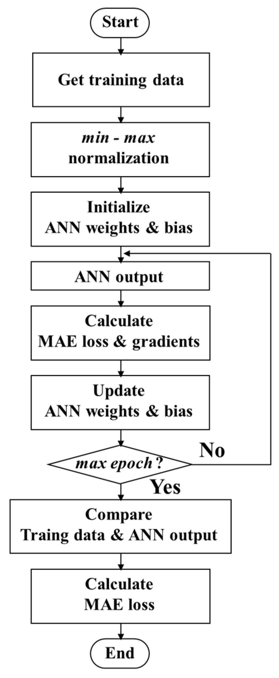
The ANN training procedure is illustrated in
Figure 2. After the PMU data acquisition and min-max normalization, the ANN weight and bias parameters are initialized. For the numerical analysis, a time-domain simulation is performed based on the Runge-Kutta method. Among all the time steps of the Runge-Kutta calculation, the data which are consistent with the PMU sampling period are adopted as the training data. The ANN trajectory output,
x’nor is obtained from (5). Based on the ANN output
x’nor and normalized training data
xnor, the MAE loss
L1 in (2) is calculated. The loss function of
L2 in (3) can also be considered if necessary. When the gradients of the total loss function
L in (1) are obtained, the ANN weight and bias values are updated using the Adam optimizer to minimize the loss function (1). This process is repeated until the number of iterations reaches the maximum number of training epochs.
3. Power System Models
3.1. WSCC 3-Machine System Model
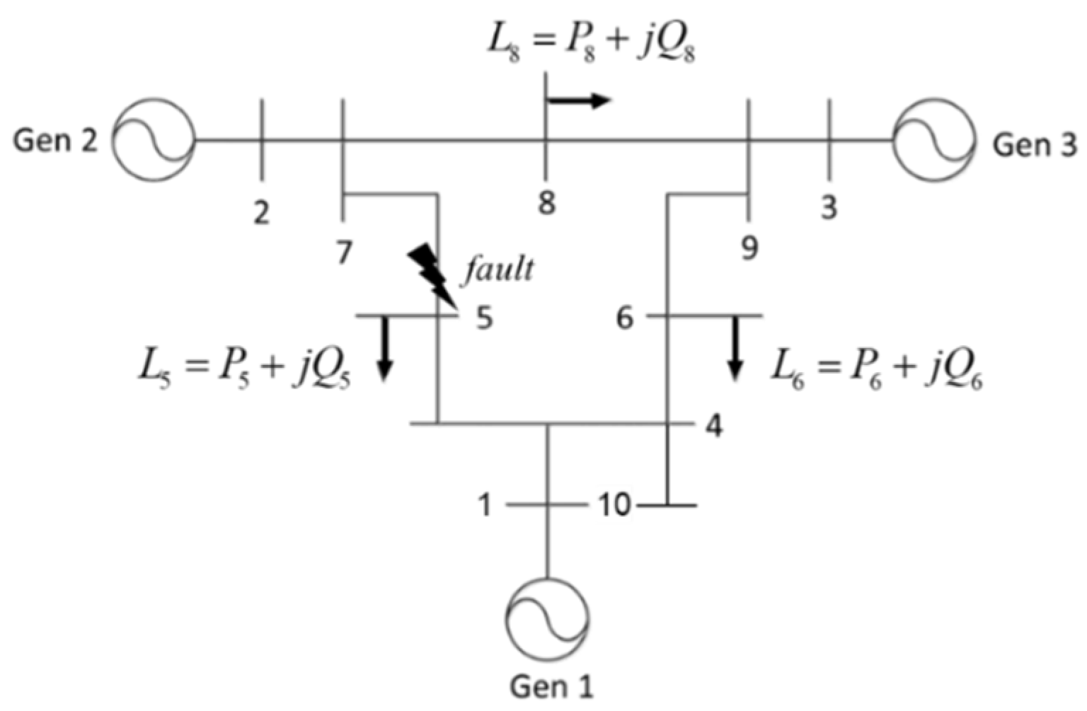
The WSCC 3-machine power system model is shown in
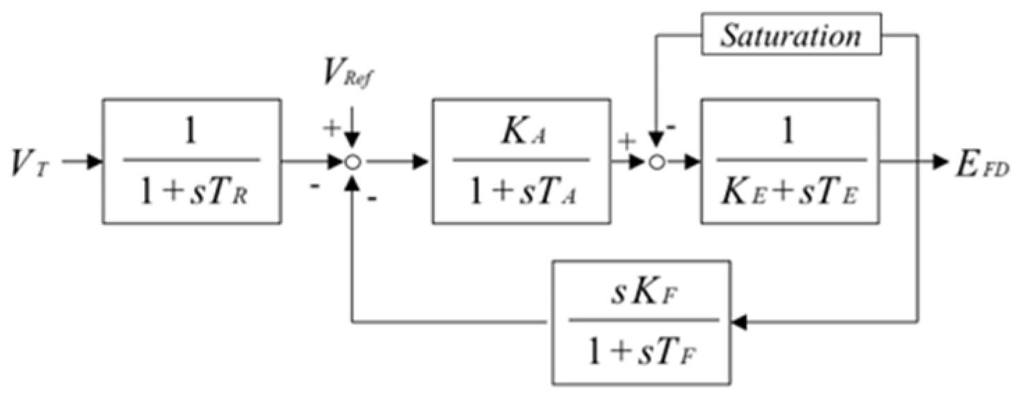
Figure 3. The three generators are equipped with their respective automatic voltage regulator (AVR) and turbine-governor (GOV) models. The IEEE Type 1 excitation model [
35] in
Figure A1 is adopted for the AVR model. The saturation effect of the AVR model is neglected. The reheated steam turbine model [
36] in
Figure A2 is applied to the turbine-governor system. The detailed configurations of the generators, AVR, and GOV models are provided in the Appendix. PMU devices are installed at all generator buses for the frequency and bus voltage measurements.
The three-phase line-to-ground fault occurrence on the transmission line between buses 5 and 7 is considered as the disturbance type. The fault is cleared after 70 ms. In the WSCC 3-machine system, ANN models are designed to predict the transient trajectories of the rotor-angle after the fault. Hence, the pre-fault rotor-angle difference between the two generators is necessary as the input data for the ANN models.
3.2. IEEE 39-Bus System Model
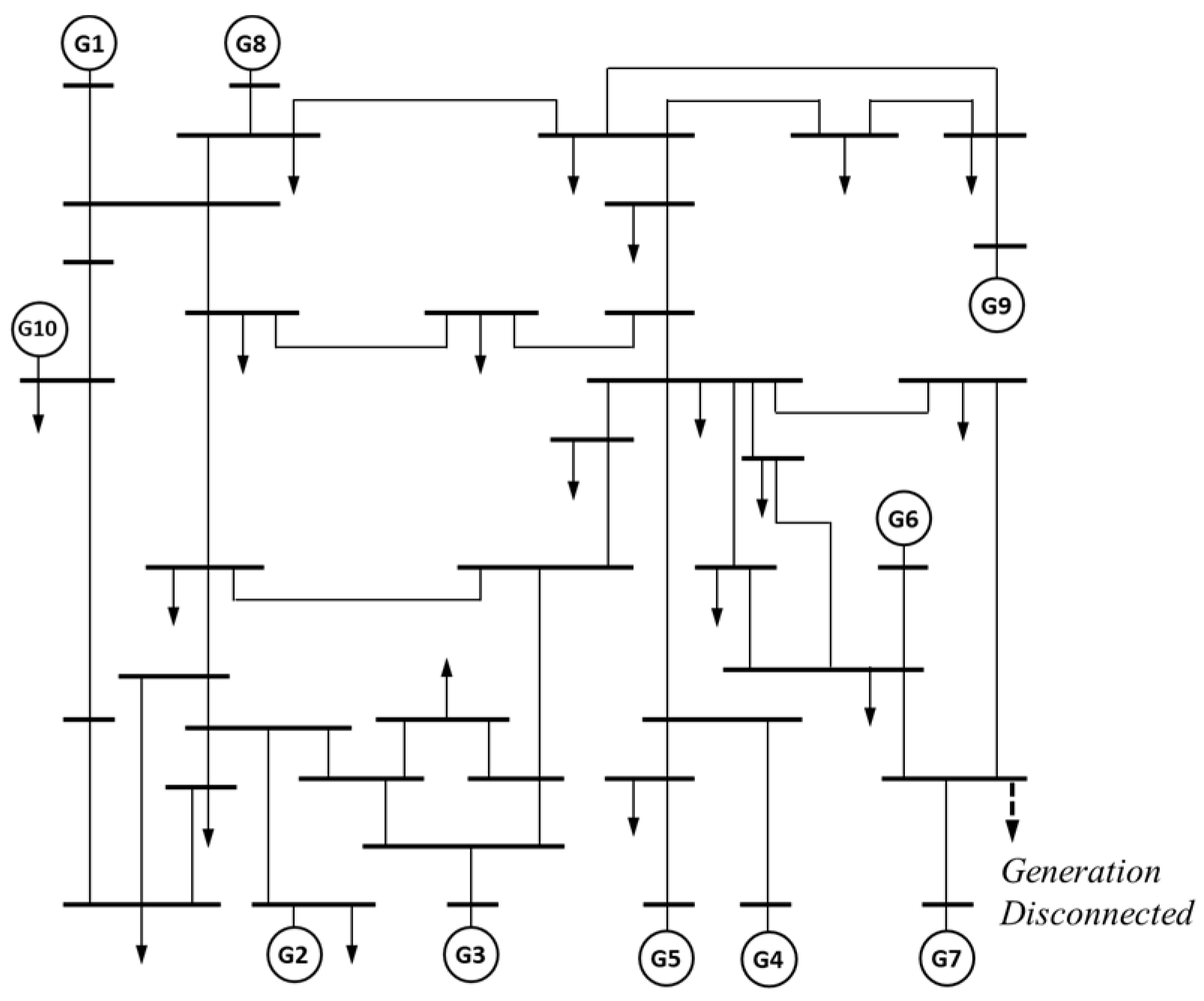
The modified IEEE 39-bus system model is described in
Figure 4. All generators have their respective AVR and GOV models, except for G10. The same IEEE Type 1 excitation [
35] and reheated steam turbine models [
36] are chosen for the AVR and GOV systems, respectively. The generators are equipped with PMU devices.
In this modified model, it is assumed that the area near G6 and G7 has high renewable energy sources potential. Thus, a new 600MW power generation source is installed in this area. For simplicity, this source is modeled as a negative static constant power load with the unity power factor.
As the disturbance type, a sudden disconnection of this generation is simulated. In this case, ANN models are responsible for evaluating the system frequency trajectory.
In a multi-machine power system model, the system frequency at the center of inertia (COI)
fCOI is the global index for frequency analysis.
fCOI is defined in (6), where G and m indicate generator G and the total number of generators, respectively. The inertia constant of the generator is represented by symbol H. The pre-disturbance input data are always 1.0 p.u. for these frequency trajectory prediction models.
4. Simulation Results
Case scenarios are classified to demonstrate the effectiveness of piecewise segment training and augmented loss function. Three cases are defined as follows:
Case 0 : No Piecewise Segment Training, L = L1
Case 1 : Piecewise Segment Training, L = L1
Case 2 : Piecewise Segment Training, L = L1 +λL2
Case 0 corresponds to the general ANN training method in which the proposed piecewise segment training and augmented loss function are not applied. In Case 1, piecewise training is adopted, but the time-derivative terms are not added to the loss function. The influence of piecewise training can be analyzed by comparing the results of Cases 0 and 1. Both piecewise segment training and augmented loss function are considered in Case 2. The ANN output differences between Cases 1 and 2 indicate the impact of the augmented loss function.
To simulate the constrained training conditions, the following training scenarios are defined depending on the number of training epochs and hidden layers:
Scenario 1 : Epoch 1000, Number of hidden layers : 2
Scenario 2 : Epoch 1500, Number of hidden layers : 3
Scenario 3 : Epoch 2000, Number of hidden layers : 4
The calculation burden is also affected by the number of neurons. Hence, sensitivity analysis on the number of neurons is required. Four cases, with different numbers of neurons, are tested. Each hidden layer has 9, 15, 21, and 30 neurons. For instance, an ANN model with 15 neurons means that the hidden layer has 15 neurons. In this case, the total number of neurons in all four hidden layers is 60 in Scenario 3.
ANN models for Case 0 are designed as explained above. In contrast, the original ANN model is divided into several sub-models in Cases 1 and 2. In such cases, each hidden layer in a sub-model has five neurons. Consequently, the ANN models in all three Cases 0, 1, and 2 have the same number of neurons.
4.1. Rotor-Angle Trajectory
After the fault occurs in the WSCC 3-machine system model, the trajectory of the rotor-angle
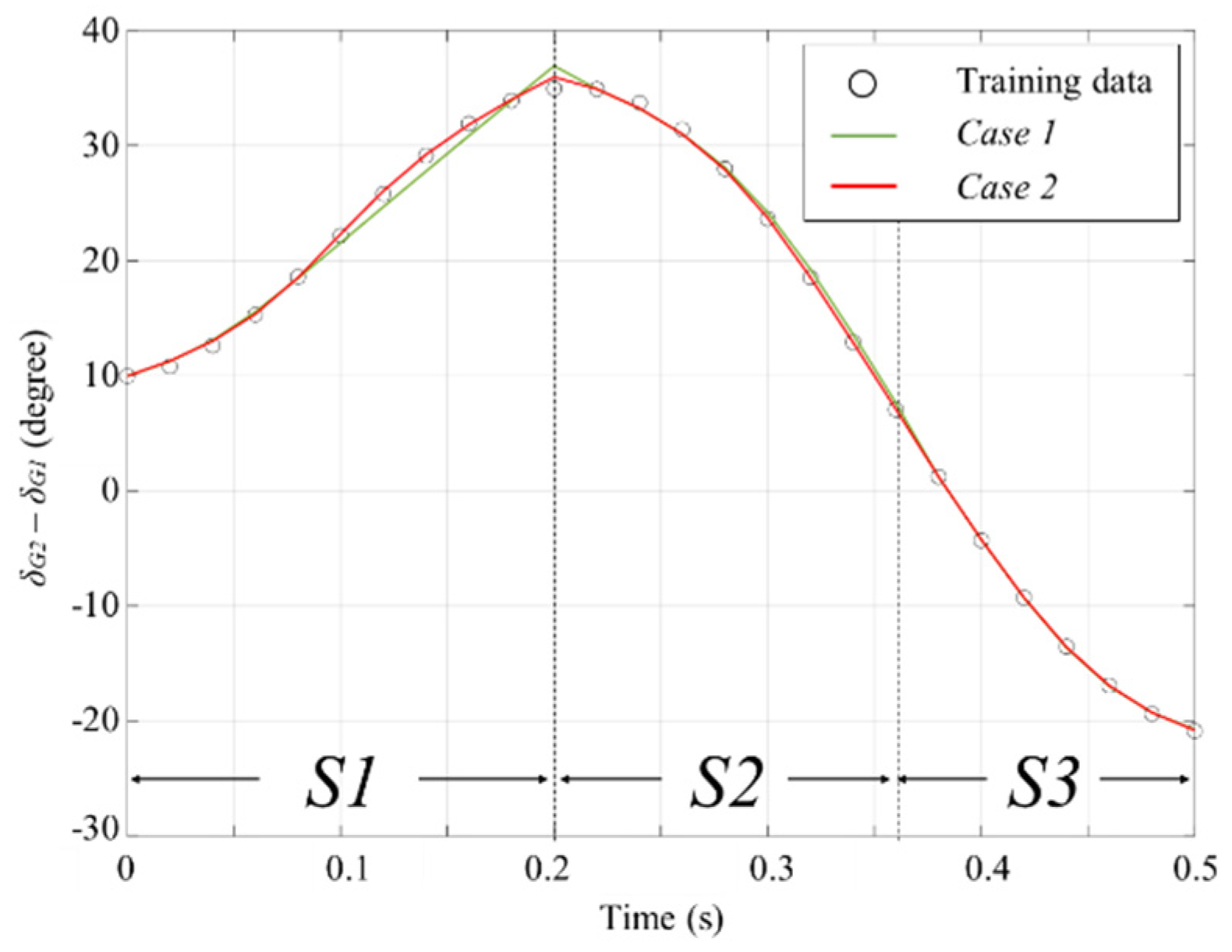
δ difference between G2 and G1 is adopted as the training data. The rotor-angle data from the initial to the minimum values are analyzed. The training data and training results of the ANN models in Scenario 3 are described in
Figure 5. The trajectory can be divided into three segments S1, S2, and S3 based on the maximum and inflection points in Cases 1 and 2, respectively. The time interval between
t =
Ni-1 and
Ni is set to be 1 ms. Due to the random characteristics of the initialization of the parameters, each ANN model is trained five times, and the average result is analyzed.
In Case 0, without piecewise segment training, the ANN model cannot be trained; thus, it is not plotted. In contrast, the training result in Case 1 is denoted by the solid green line. Therefore, it can be inferred that piecewise segment training is valid for training the rotor-angle trajectory models. Furthermore, it is noteworthy that the training result in Case 2 is closer to the original training data than those in Case 1. Based on this difference, the effectiveness of the augmented loss function method can be verified.
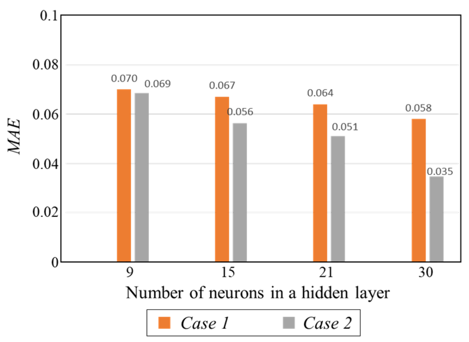
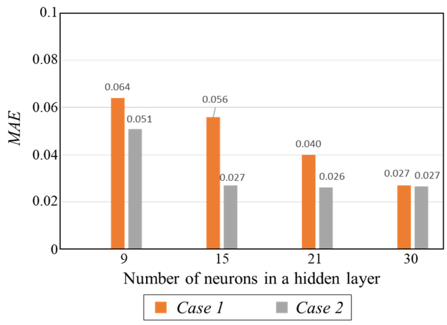
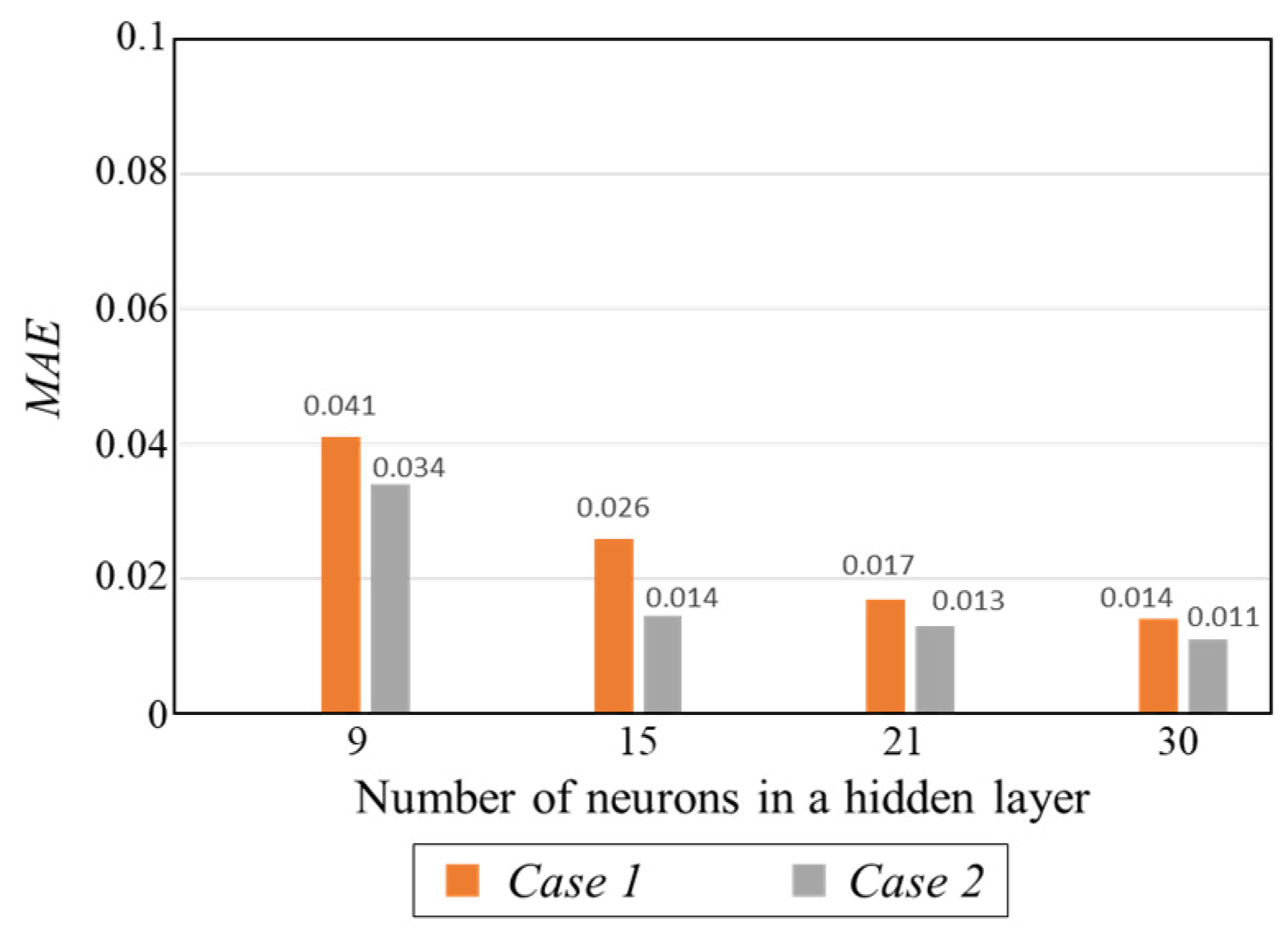
The performance of the training process is evaluated based on MAE loss values. The MAE losses in the three training scenarios are listed from
Figure 6,
Figure 7 and
Figure 8. The values on the horizontal axis indicate the number of neurons in a hidden layer. For example, the number ‘9’ corresponds to an ANN model with nine neurons in a hidden layer. In this case, the total number of neurons in all the hidden layers is 18 in Scenario 1.
As shown in
Figure 6, with nine neurons for each hidden layer, the ANN models cannot be trained effectively in both Cases 1 and 2. Hence, the highest MAE losses are observed in both cases. The MAE values can be reduced as the number of neurons increases.
It should be noted that in Scenario 1, when the neuron number increases, the MAE reduction effect in Case 2 is larger than that in Case 1. This demonstrates the validity of the augmented loss function method in Scenario 1. In particular, the impact of augmented loss function is the largest, with 30 neurons in Scenario 1. Similar to these results, the MAE losses also decrease if the neuron number increases, as notated in
Figure 7 and
Figure 8.
Owing to the augmented loss function, the MAE values in Case 2 can be reduced compared to the results in Case 1 in Scenarios 2 and 3.
Unlike Scenario 1, different tendencies are observed in Scenarios 2 and 3. In Scenario 2, the MAE results show almost no difference between Cases 1 and 2 when the number of neurons in a hidden layer is 30 in
Figure 7. The MAE difference between Cases 1 and 2, with 21 neurons for each hidden layer, is lower than that with 15 neurons. On top of that, the largest MAE reduction in Case 2 is obtained by the model with 15 neurons for each hidden layer in
Figure 8, Scenario 3. The MAE differences in Scenario 3 are relatively insignificant compared with the results in Scenario 2.
These results imply that the augmented loss function method is effective in reducing the MAE loss values when the training epoch and neuron numbers are constrained.
4.2. Frequency Trajectory
Considering the generation disconnection in the modified IEEE 39-bus system model, the system frequency at the center of inertia
fCOI is used as the training data. The frequency data from the initial value to the frequency nadir point is investigated. In
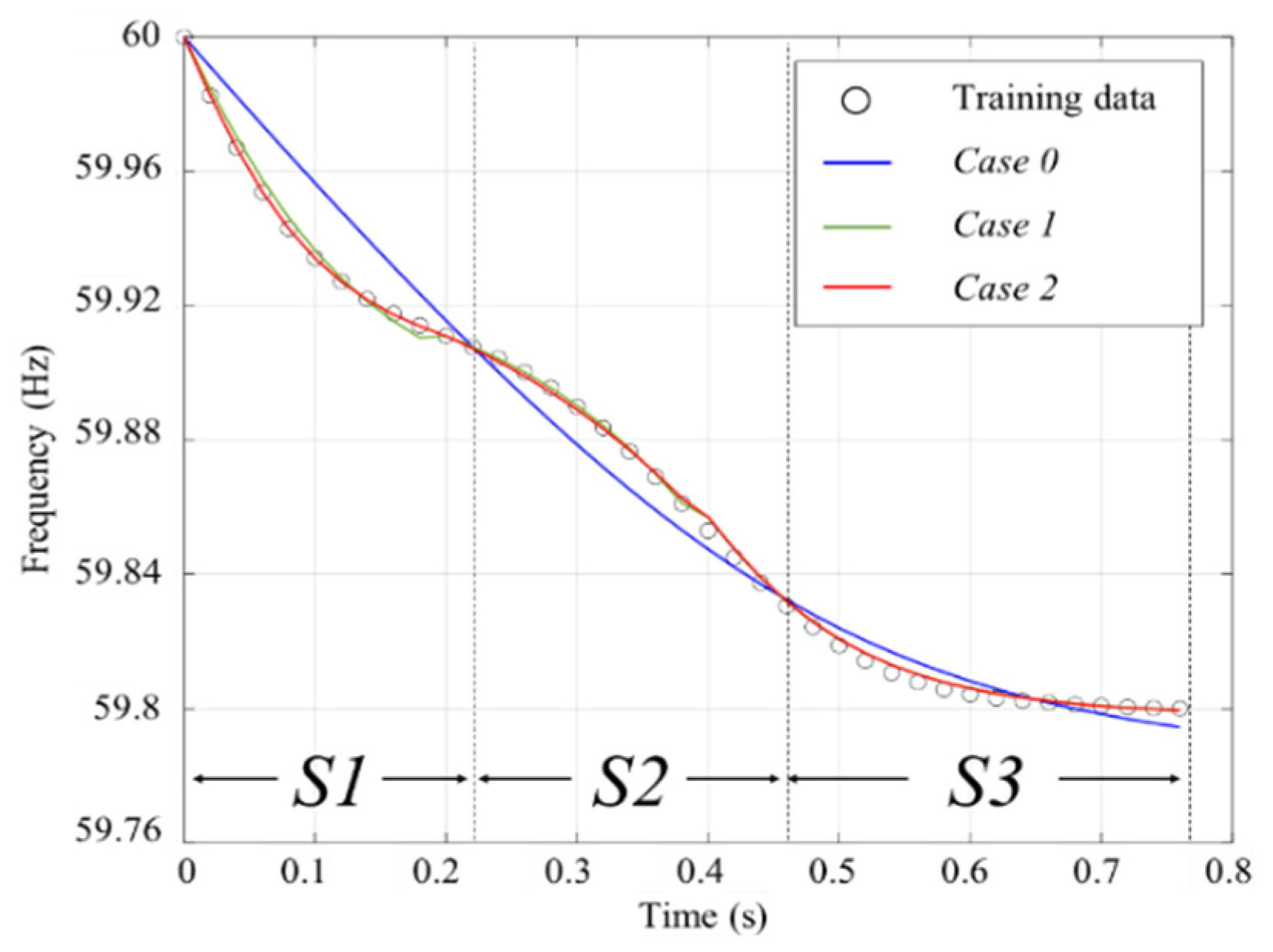
Figure 9, the training data and the results of the ANN training models with 15 neurons for each hidden layer in Scenario 1 are shown as representative examples. The original training problem is split into sub-problems S1, S2, and S3 in Cases 1 and 2. The boundaries of these sub-problems are determined by the two inflection points of the
fCOI trajectory. The ANN models are trained with 1 ms time interval. Similar to the analysis in the WSCC 3-machine system, all ANN models are tested five times considering the random initialization of the ANN parameters.
It can be seen that the ANN model is not well-trained in Case 0. This implies that without piecewise segment training and augmented loss methods, the training epoch and neuron number constraints in Scenario 1 are severe conditions. On the other hand, the training results of the ANN models in Cases 1 and 2 show relatively better performance. In particular, the best training result among the three cases is obtained in Case 2. Therefore, the proposed methods are also valid for the frequency fCOI trajectory prediction.
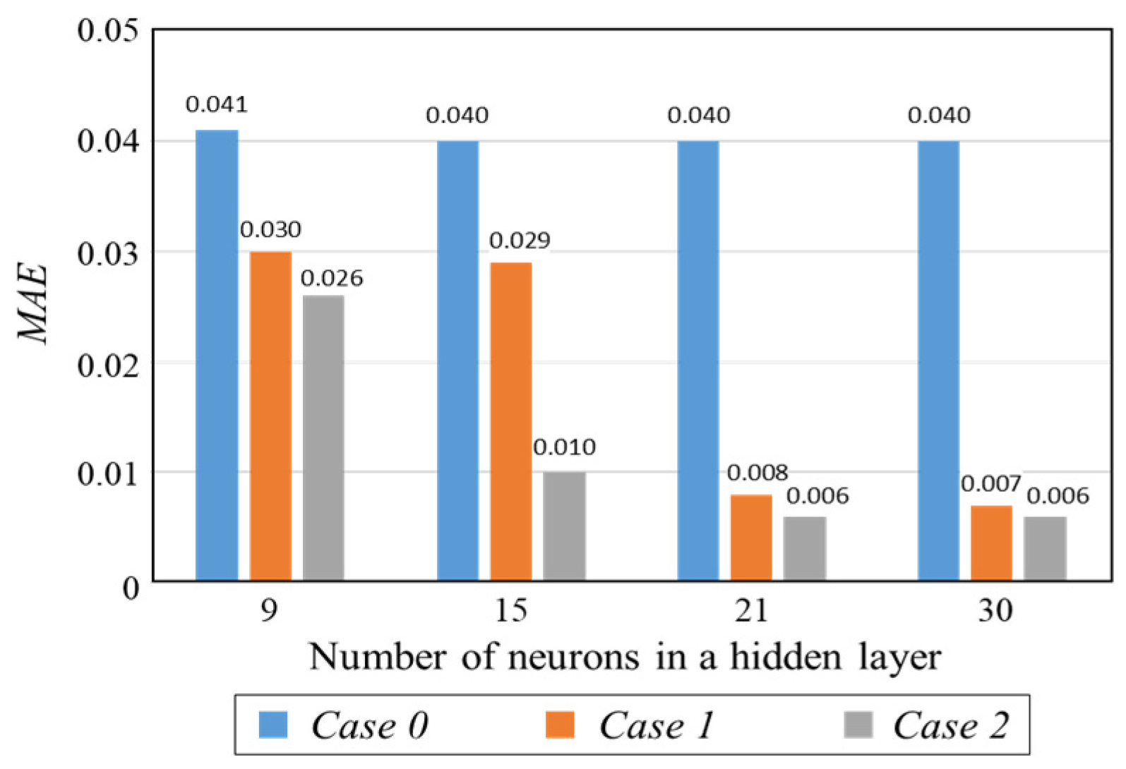
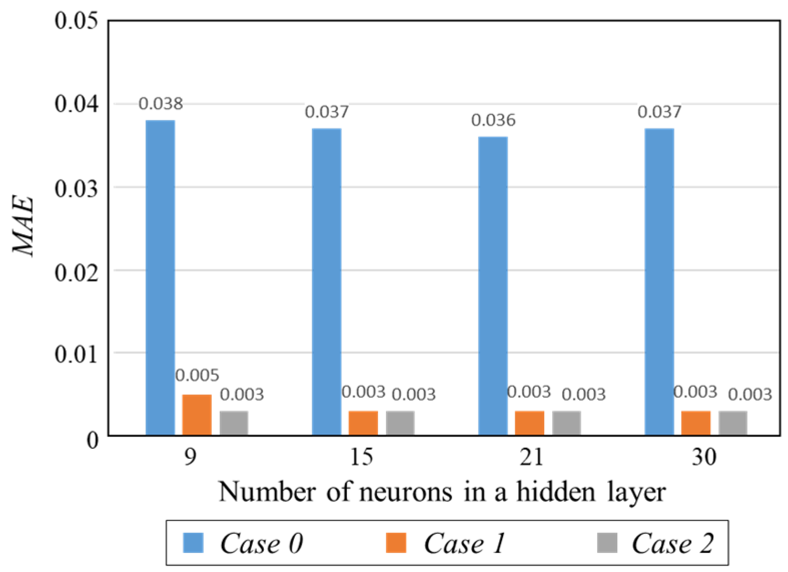
The MAE losses of the ANN frequency trajectory prediction models in Scenarios 1 and 2 are depicted in
Figure 10 and
Figure 11, respectively. The preliminary study revealed that in Scenario 3, the lowest MAE value can be obtained in both Cases 1 and 2; thus, it is not discussed here.
In Scenario 1, the largest MAE losses are observed in Case 0 among all three cases. It should be noted that in Case 0, there is almost no loss difference even when the neuron number increases. Therefore, it can be inferred that the ANN frequency prediction model cannot be effectively trained without the proposed piecewise segment training and augmented loss function in Scenario 1.
Compared with the results in Case 0, the MAE losses in Case 1 are reduced if the same number of neurons is provided for ANN models. This validates the effectiveness of piecewise segment training in the frequency trajectory prediction model. Similarly, the MAE values in Case 2 can be decreased compared with those in Case 1, which indicates the validity of the augmented loss function.
Although the lowest MAE loss is calculated in Case 2, the result is 0.026, which is still not small when the number of neurons in a hidden layer is nine. The MAE loss difference between Cases 1 and 2 is the largest with 15 neurons in a hidden layer. On the contrary, the difference is relatively not significant with more than 21 neurons in a hidden layer. This implies that if the ANN models have sufficient neurons, the Case 1 method is sufficient for training the ANN frequency prediction model. In other words, the augmented loss method in Case 2 is the most effective when the number of neurons for each hidden layer is constrained to 15.
In Scenario 2, the MAE losses in Case 0 have the largest values among all three cases. Even if the number of neurons increases, these losses cannot be reduced, which shows a tendency similar to the results in Scenario 1.
Compared to these losses, lower MAE values are calculated for Cases 1 and 2. If each hidden layer of the ANN model has more than 15 neurons, the lowest MAE loss of 0.003 is obtained. Especially, the MAE loss in Case 1 is 0.005 with nine neurons in a hidden layer. These MAE results indicate that the ANN models can be trained well in Case 1. This is because the numbers of training epochs and neurons are increased in Scenario 2. In this training scenario, the piecewise segment training method in Case 1 is sufficient to train the ANN model. The impact of augmented loss in Scenario 2 is not as effective as that in Scenario 1.
5. Conclusions
ANN training improvement methods for trajectory prediction models are developed in this paper. The original trajectory training can be divided into several sub-segments. The boundaries of the segments are determined based on the maximum, minimum, and inflection points of the original trajectory. Furthermore, an augmented loss function method is proposed. In addition to the MAE value, the time-derivative terms of the training data and ANN output are included in the augmented loss function. The validity of the training improvement methods is verified for rotor-angle and frequency trajectory predictions in power system models. The numerical analysis has shown that the proposed techniques are effective and can reduce MAE losses when the training epoch and neuron numbers are constrained. With the constrained training conditions, the impact of reducing redundant connections among neurons and reshaping the structure of ANN models is valuable for the future investigation. Based on these accomplishments, hybrid models consisting of an ANN and other AI models can be studied in the future. The sensitivity analysis on different PMU data sampling frequencies will also be covered.
Author Contributions
Conceptualization, methodology, software, validation, formal analysis, investigation, resources, data curation, writing—original draft preparation, writing—review and editing, and visualization, H.S.; supervision, G.J. All authors have read and agreed to the published version of the manuscript.
Funding
This work was supported by the National Research Foundation of Korea (NRF) grant funded by the Korean Government (MSIT) under Grant RS-2022-00165574.
Data Availability Statement
Not applicable.
Conflicts of Interest
The authors declare no conflict of interest.
Appendix
Figure A1.
IEEE Type 1 excitation model [
35].
Figure A1.
IEEE Type 1 excitation model [
35].
Figure A2.
Turbine-governor model (reheated steam type) [
36].
Figure A2.
Turbine-governor model (reheated steam type) [
36].
Table A1.
Generator Parameters of WSCC 3-Machine System.
Table A1.
Generator Parameters of WSCC 3-Machine System.
Table A2.
AVR Parameters of WSCC 3-Machine System.
Table A2.
AVR Parameters of WSCC 3-Machine System.
Table A3.
Turbine-Governor Parameters of WSCC 3-Machine System.
Table A3.
Turbine-Governor Parameters of WSCC 3-Machine System.
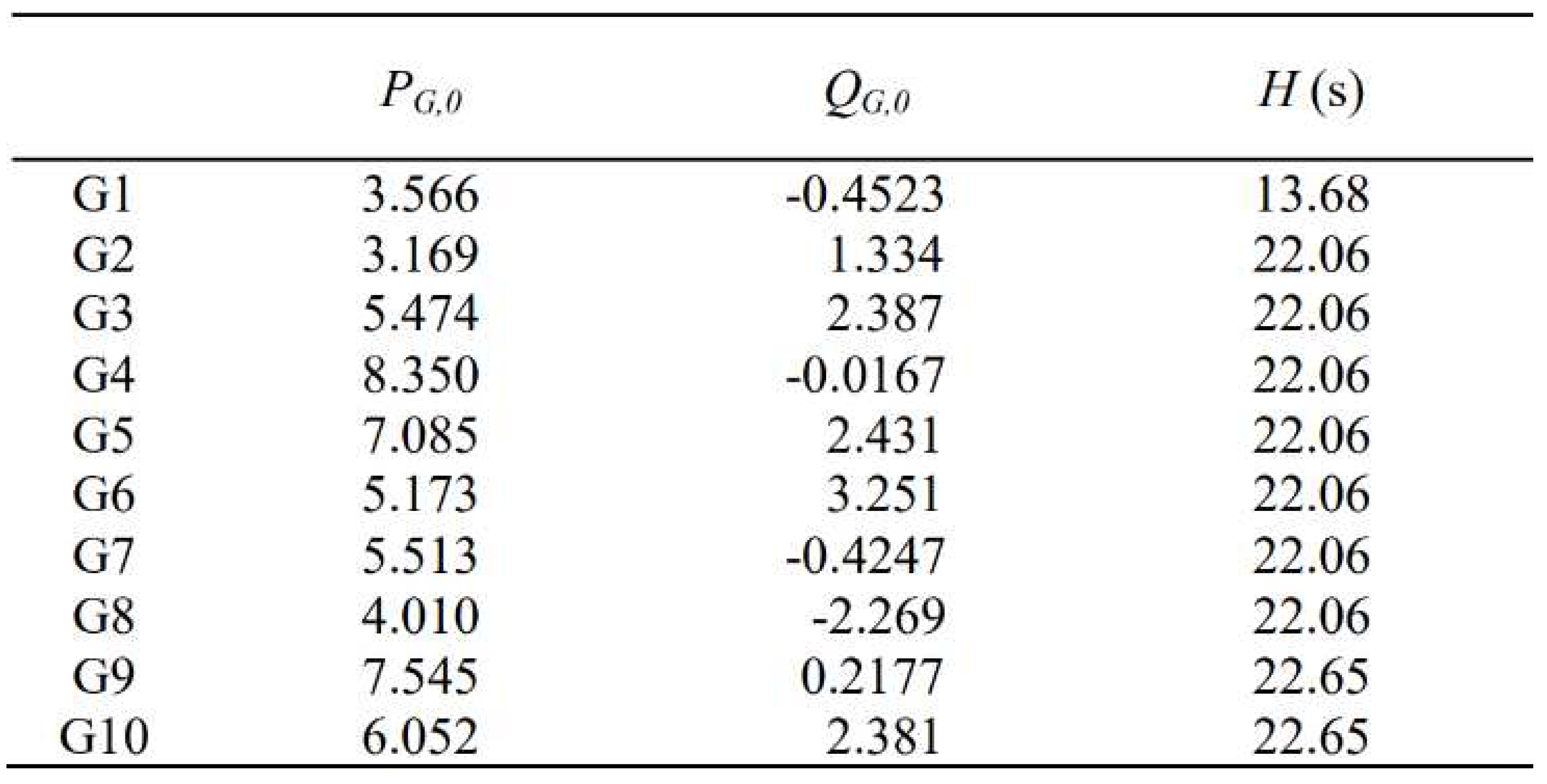
Table A4.
Generator Parameters of IEEE 10-Machine System.
Table A4.
Generator Parameters of IEEE 10-Machine System.
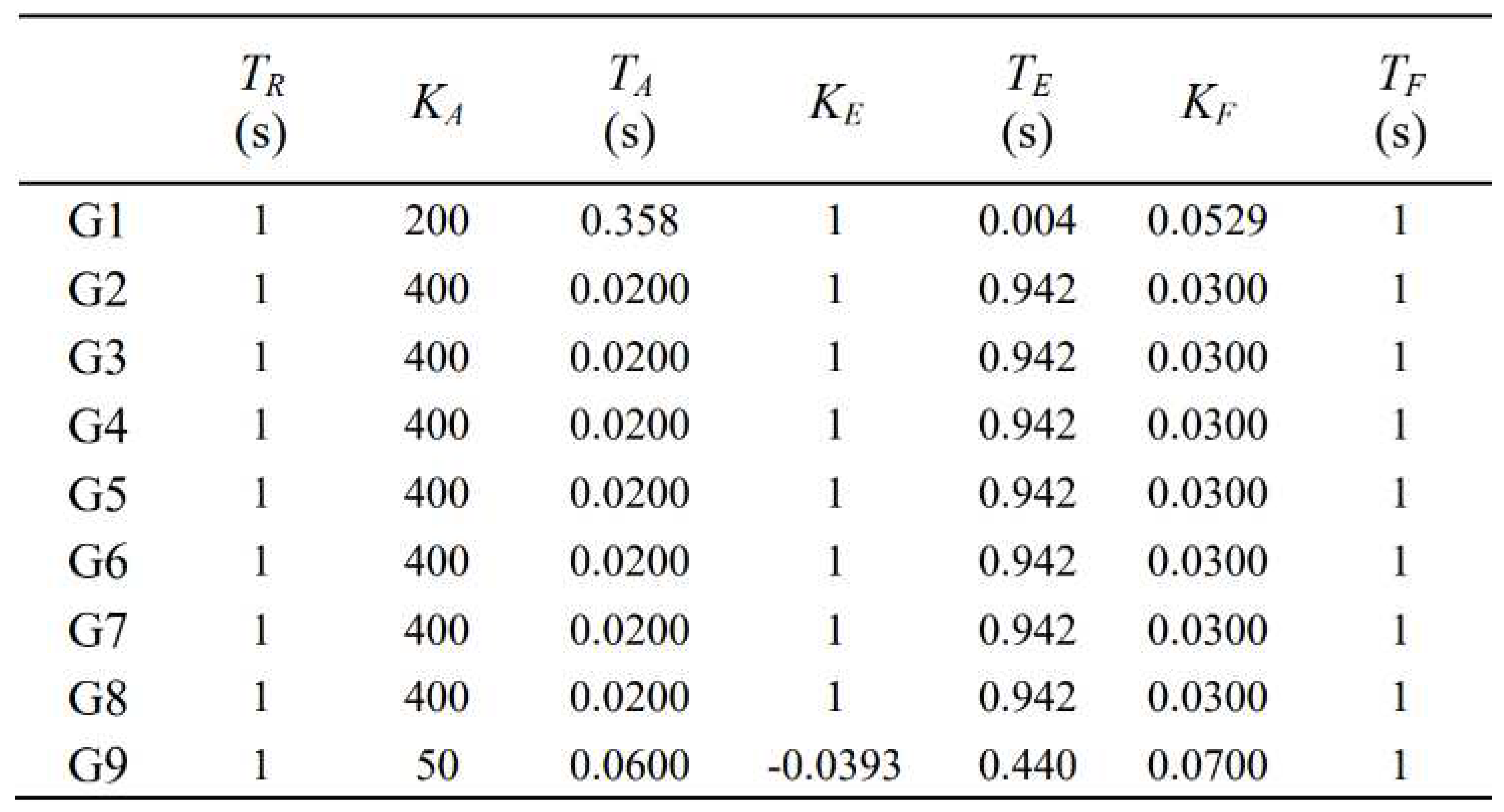
Table A5.
AVR Parameters of IEEE 10-Machine System.
Table A5.
AVR Parameters of IEEE 10-Machine System.
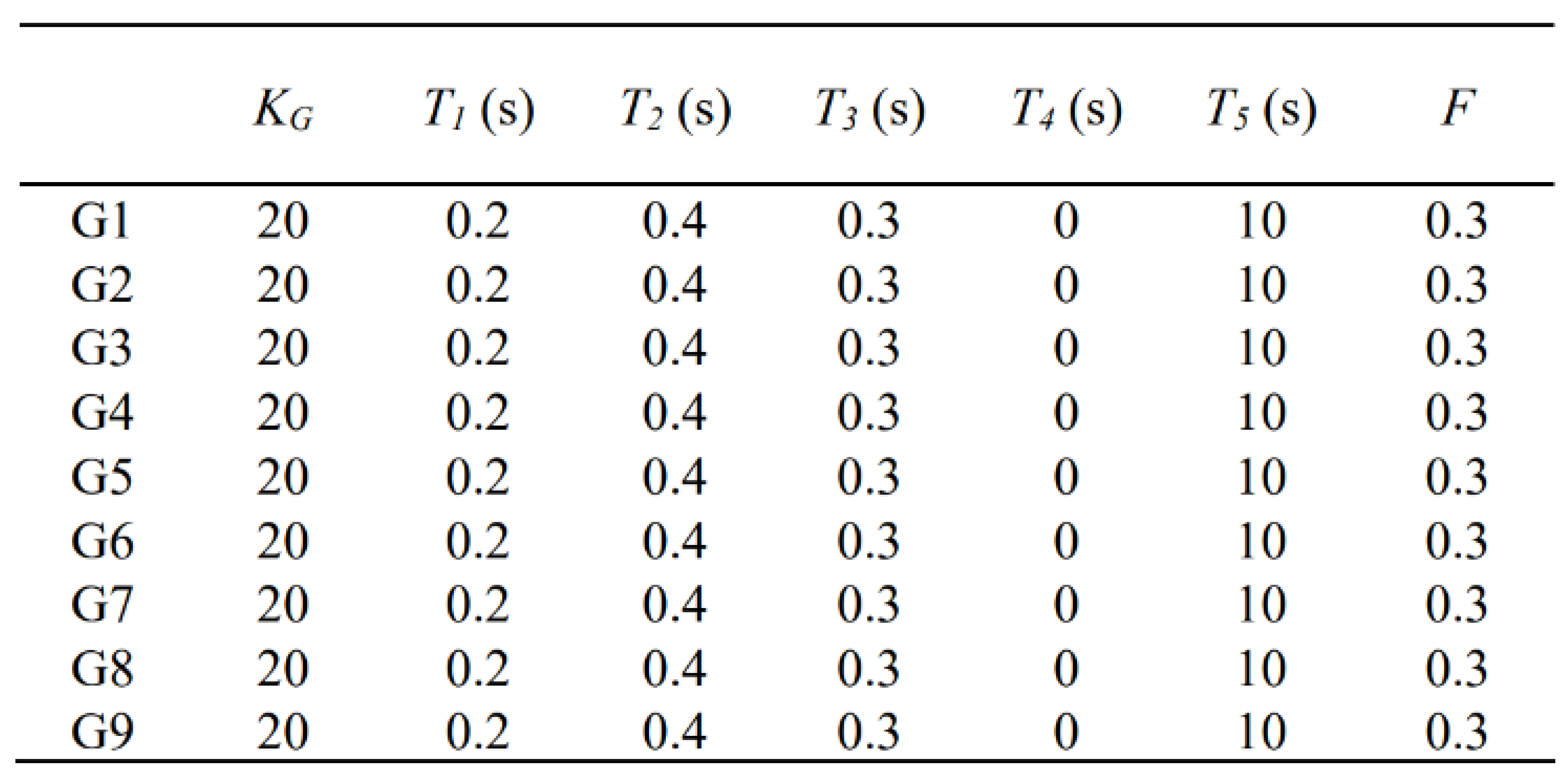
Table A6.
Turbine-Governor Parameters of IEEE 10-Machine System.
Table A6.
Turbine-Governor Parameters of IEEE 10-Machine System.
References
- V. Malbasa; C. Zheng; P. Chen; T. Popovic; Mladen Kezunovic. Voltage Stability Prediction Using Active Machine Learning. IEEE Trans. Smart Grid. 2017, 8, 3117–3124. [CrossRef]
- IEEE Standard for Synchrophasor Measurements for Power Systems, IEEE Standard C37.118.1-2011, 2011, pp. 1–61.
- P. Gupta; S. A. Soman. Calibrating CVTs of a Substation From Local PMU Data: An SVD Approach. IEEE Trans. Power Syst. 2021, 36, 3362–3371. [CrossRef]
- B. D. Tan; J. Yang; Y. F. Tang; S. B. Jiang; P. Y. Xie; W. Yuan. A deep imbalanced learning framework for transient stability assessment of power system. IEEE Access. 2019, 7, 81759–81769. [CrossRef]
- S. L. Zhang; Y. X. Wang; M. Q. Liu; Z. J. Bao. Data-based line trip fault prediction in power systems using LSTM networks and SVM. IEEE Access. 2017, 6, 7675–7686. [CrossRef]
- E. Yeung; S. Kundu; N. Hodas. Learning deep neural network representations for koopman operators of nonlinear dynamical systems. In 2019 American Control Conference (ACC), Philadelphia, PA, USA, 10-12 July 2019.
- R. Yousefian; S. Kamalasadan. Energy function inspired value priority based global wide-area control of power grid. IEEE Trans. Smart Grid. 2018, 9, 552–563. [CrossRef]
- Z. Ping; Z. Yin; X. Li; Y. Liu; T. Yang. Deep koopman model predictive control for enhancing transient stability in power grids. International Journal of Robust and Nonlinear Control. 2021, 31, 1964–1978. [CrossRef]
- P. You; J. Pang; E. Yeung. Deep koopman controller synthesis for cyber-resilient market-based frequency regulation. IFAC-PapersOnLine. 2018, 51, 720–725. [CrossRef]
- J. Sun; Z. Zhu; H. Li; Y. Chai; G. Qi; H. Wang; Y. H. Hu. An integrated critic-actor neural network for reinforcement learning with application of ders control in grid frequency regulation. International Journal of Electrical Power & Energy Systems. 2019, 111, 286-299. [CrossRef]
- M. Khodayar; O. Kaynak; M. E. Khodayar. Rough deep neural architecture for short-term wind speed forecasting. IEEE Trans. on Industrial Informatics. 2017, 13, 2770–2779. [CrossRef]
- J. Yan; H. Zhang; Y. Q. Liu; S. Han; L. Li; Z. X. Lu. Forecasting the high penetration of wind power on multiple scales using multi-tomulti mapping. IEEE Trans. on Power Syst. 2018, 33, 3276–3284. [CrossRef]
- H. X. Zhou; Y. J. Zhang; L. F. Yang; Q. Liu; K. Yan; Y. Du. Short-term photovoltaic power forecasting based on long short term memory neural network and attention mechanism. IEEE Access. 2019, 7, 78063–78074. [CrossRef]
- Z. X. Sun; S. S. Zhao; J. X. Zhang. Short-term wind power forecasting on multiple scales using VMD decomposition, k-means clustering and LSTM principal computing. IEEE Access. 2019, 7, 166917–166929. [CrossRef]
- M. Khodayar; S. Mohammadi; M. E. Khodayar; J. H. Wang; G. Y. Liu. Convolutional graph autoencoder: a generative deep neural network for probabilistic spatio-temporal solar irradiance forecasting. IEEE Trans. on Sustainable Energy. 2020, 11, 571–583. [CrossRef]
- M. Tan; S. P. Yuan; S. H. Li; Y. X. Su; H. Li; F. He. Ultra-short-term industrial power demand forecasting using LSTM based hybrid ensemble learning. IEEE Trans. on Power Syst. 2020, 35, 2937–2948. [CrossRef]
- J. Dong; X. Ma; S. M. Djouadi; H. Li; Y. Liu. Frequency prediction of power systems in FNET based on state-space approach and uncertain basis functions. IEEE Trans. on Power Syst. 2014, 29, 2602–2612. [CrossRef]
- H. Ma; H. Li. Analysis of frequency dynamics in power grid: A Bayesian structure learning approach. IEEE Trans. on Smart Grid. 2013, 4, 457–466. [CrossRef]
- S. Kaur; S. Agrawal; Y. P. Verma. Power grid frequency prediction using ANN considering the stochasticity of wind power. In 2013 5th International Conference and Computational Intelligence and Communication Networks, Mathura, India, 27-29 September 2013.
- A. Bolzoni; R. Todd; A. Forsyth; R. Perini. Real-time auto-regressive modelling of electric power network frequency. In IECON 2019 - 45th Annual Conference of the IEEE Industrial Electronics Society, Lisbon, Portugal, 14-17 October 2019.
- W. Bang; J. W. Yoon. Forecasting the electric network frequency signals on power grid. In Forecasting the electric network frequency signals on power grid, Jeju, South Korea, 16-18 October 2019.
- U. Rudez; R. Mihalic. WAMS-Based Underfrequency Load Shedding With Short-Term Frequency Prediction. IEEE Trans. on Power Delivery. 2016, 31, 1912-1920. [CrossRef]
- Y. JEONG; S. KIM; K. YI. Surround Vehicle Motion Prediction Using LSTM-RNN for Motion Planning of Autonomous Vehicles at Multi-Lane Turn Intersections. IEEE Open Journal of Untelligent Transportatin Systems. 2020, 1, 2-14. [CrossRef]
- C. Yang; C. Wu; J. Shao; Y. Wang; C. Hsieh. AIS-Based Intelligent Vessel Trajectory Prediction Using Bi-LSTM. IEEE Access. 2022, 10, 24302-24315. [CrossRef]
- L. Ma; S. Tian. A Hybrid CNN-LSTM Model for Aircraft 4D Trajectory Prediction. IEEE Access. 2020, 8, 134668-134680. [CrossRef]
- Z. Shi; M. Xu; Q. Pan. 4-D Flight Trajectory Prediction With Constrained LSTM Network. IEEE Trans. on Intelligent Transportation Systems. 2021, 22, 7242-7255. [CrossRef]
- H. Xue; D. Q. Huynh; M. Reynolds. A Location-Velocity-Temporal Attention LSTM Model for Pedestrian Trajectory Prediction. IEEE Access. 2020, 8, 44576-44589. [CrossRef]
- H. Xue; D. Q. Huynh; M. Reynolds. PoPPL: Pedestrian Trajectory Prediction by LSTM With Automatic Route Class Clustering. IEEE Trans. on Neural Networks and Learning Systems. 2021, 32, 77-90. [CrossRef]
- L. Xie; Z. We; D. Ding; Z. Zhang; A. Tang. Long and Short Term Maneuver Trajectory Prediction of UCAV Based on Deep Learning. IEEE Access. 2021, 9, 32321-32340. [CrossRef]
- I. E. Lagaris; A. Likas; D. I. Fotiadis. Artificial Neural Networks for Solving Ordinary and Partial Differential Equation. IEEE Trans. Neural Networks. 1998, 9, 987-1000. [CrossRef]
- L. Shalalfeh; P. Bogdan; E. A. Jonckheere. Fractional Dynamics of PMU Data. IEEE Trans. Smart Grid. 2021, 12, 2578-2588. [CrossRef]
- M. Lahariya; F. Karami; C. Develde; G. Crevecoeur. Physics-informed Recurrent Neural Networks for The Identification of a Generic Energy Buffer System. In 2021 IEEE 10th Data Driven Control and Learning Systems Conference (DDCLS), Suzhou, China, 14-16 May 2021.
- R. Nellikkath; S. Chatzivasileiadis. Physics-Informed Neural Networks for AC Optimal Power Flow. Electric Power Systems Research. 2022, 212, 108412-108418. [CrossRef]
- S. Kim. Improving ANN Training with Approximation Techniques for ROCOF Trajectory Estimation. In 2023 IEEE Belgrade PowerTech, Belgrade, Serbia, 25-29 June 2023.
- P. Demetriou; M. Jairo; Q. Tortos; E. Kyriakides. Dynamic IEEE Test Systems for Transient Analysis. IEEE Systems Journal. 2017, 11, 2108-2117. [CrossRef]
- X. Zhao; H. Wei; J. Qi; P. Li; X. Bai. Frequency Stability Constrained Optimal Power Flow Incorporating Differential Algebraic Equations of Governor Dynamics. IEEE Trans. on Power Systems. 2021, 36, 1666-1676. [CrossRef]
|
Disclaimer/Publisher’s Note: The statements, opinions and data contained in all publications are solely those of the individual author(s) and contributor(s) and not of MDPI and/or the editor(s). MDPI and/or the editor(s) disclaim responsibility for any injury to people or property resulting from any ideas, methods, instructions or products referred to in the content. |
© 2024 by the authors. Licensee MDPI, Basel, Switzerland. This article is an open access article distributed under the terms and conditions of the Creative Commons Attribution (CC BY) license (http://creativecommons.org/licenses/by/4.0/).
