Restricted Singular Value Decomposition for a Tensor Triplet under T-product and Its Applications

Preprint

Article

Restricted Singular Value Decomposition for a Tensor Triplet under T-product and Its Applications

Altmetrics

Downloads

114

Views

Comments

A peer-reviewed article of this preprint also exists.

Chong-Quan Zhang

Qing-Wen Wang^*,Xiang-Xiang Wang,

Zhuo-Heng He

Chong-Quan Zhang

Qing-Wen Wang^*,Xiang-Xiang Wang,

Zhuo-Heng He

This version is not peer-reviewed

Submitted:

08 February 2024

Posted:

09 February 2024

You are already at the latest version

Alerts

Abstract

We investigate and discuss in detail the structure of the restricted singular value decomposition for a tensor triplet under t-product (T-RSVD). The algorithm is provided with a numerical example illustrating the main result. For applications, we consider color image watermarking processing with T-RSVD.

Keywords:

Subject: Physical Sciences - Mathematical Physics

MSC: 15A23; 15A69; 65F30

1. Introduction

A great number of problems lead to decompositions of higher-order tensors; examples include color image processing, genomic signals, higher-order statistics, pattern recognition, chemometrics, aerospace engineering, etc . (see e.g., [2,5,8,9,17,18,19,20] and references therein). There have been many papers discussing tensor decompositions under various tensor products ([3,8,12,15,21,22]).

Some well-known multiplications of tensors are the n-mode, Kronecker, Khatri–Rao and Einstein products. The t-product is a new type of tensor multiplication that can be used in imaging (see e.g., [6,8,10,13]). Kilmer and Martin [11] investigated the tensor singular value decomposition under t-product (T-SVD) for third-order tensors. Martin et al. [13] extended the T-SVD to order-p tensors. Very recently, He et al. [8] considered the generalized singular value decompositions for two tensors via the t-product.

To our knowledge, there is little information on the decompositions for three tensors under t-product. Motivated by the wide applications of tensor decompositions in order to improve the theoretical development of tensor decompositions, we consider the restricted singular value decomposition (T-RSVD) for three tensors under t-product. One goal of this article is to investigate and discuss the structure and algorithm of T-RSVD. Another goal is to give an application in color image watermarking processing.

The remainder of the paper is organized as follows. In Section 2, we review some definitions, notations and background used throughout the paper. In Section 3, we derive the structure and properties of T-RSVD. We present an algorithm and a numerical example to illustrate the main result. We give an application on color image watermarking processing in Section 4.

2. Preliminaries

An order three dimension

n_{1} \times n_{2} \times n_{3}

tensor

A = (a_{i_{1} i_{2} i_{3}}) \in C^{n_{1} \times n_{2} \times n_{3}}

is a multidimensional array with

n_{1} n_{2} n_{3}

entries. Let

C^{n_{1} \times n_{2} \times n_{3}}

be the set of all order three dimension

n_{1} \times n_{2} \times n_{3}

tensors over the complex number field

C

A = (a_{i_{1} i_{2} i_{3}}) \in C^{n_{1} \times n_{2} \times n_{3}}

with

n_{1} \times n_{2}

frontal slices

A_{1}, \dots, A_{n_{3}}

, then

\begin{matrix} unfold (A) = [\begin{matrix} A_{1} \\ A_{2} \\ ⋮ \\ A_{n_{3}} \end{matrix}], \end{matrix}

(1)

\begin{matrix} bcirc (A) = [\begin{matrix} A_{1} & A_{n_{3}} & A_{n_{3} - 1} & \dots & A_{2} \\ A_{2} & A_{1} & A_{n_{3}} & \dots & A_{3} \\ ⋮ & ⋮ & ⋮ & ⋱ & ⋮ \\ A_{n_{3}} & A_{n_{3} - 1} & A_{n_{3} - 2} & \dots & A_{1} \end{matrix}], \end{matrix}

(2)

where

A_{i} = A (:, :, i)

for

i = 1, \dots, n_{3} .

The operations

fold (\cdot)

and

{bcirc}^{- 1} (\cdot)

take (1) and (2) back to an

n_{1} \times n_{2} \times n_{3}

tensor. That means

\begin{matrix} fold (unfold (A)) = A, {bcirc}^{- 1} (bcirc (A)) = A . \end{matrix}

Note that

\begin{matrix} (F_{n_{3}} \otimes I_{n_{1}}) bcirc (A) (F_{n_{3}}^{*} \otimes I_{n_{2}}) = diag (D_{1}, \dots, D_{n_{3}}), \end{matrix}

(3)

where

F_{n_{3}}^{*}

is the conjugate transpose of

n_{3} \times n_{3}

normalized discrete Fourier transformation (DFT) matrix

F_{n_{3}}

, and ⊗ denotes the Kronecker product of matrices. The matrices

D_{1}, \dots, D_{n_{3}}

are diagonal (sub-diagonal, upper-triangular, lower-triangular) if and only if the matrices

A_{1}, \dots, A_{n_{3}}

are diagonal (sub-diagonal, upper-triangular, lower-triangular) [14], and

\begin{matrix} A_{i} = \sum_{j = 1}^{n_{3}} ω^{(j - 1) (i - 1)} D_{j}, i = 1, \dots, n_{3}, \end{matrix}

(4)

where

ω = e^{- 2 π i / n_{3}}

is a primitive

n_{3}

th root of unity.

The definitions of t-product of two tensors, identity tensor, conjugate transpose, inverse tensor and unitary tensor are given as follows.

Definition 1

(t-product of third-order tensors [11]). Let

A \in C^{n_{1} \times n_{2} \times n_{3}}

and

B \in C^{n_{2} \times l \times n_{3}}

be given. Then the t-product

A * B \in C^{n_{1} \times l \times n_{3}}

is defined as

\begin{matrix} A * B = fold (bcirc (A) unfold (B)) . \end{matrix}

(5)

Definition 2

(Identity tensor [11]). The identity tensor

I \in C^{m \times m \times n}

is defined to be a tensor whose first frontal slice is the

m \times m

identity matrix and whose other frontal sliced are zero matrices, i.e.,

bcirc (I) = I_{m n}

Definition 3

(Conjugate transpose [11]). For a given tensor

A \in C^{l \times m \times n}

A^{*}

is the

m \times l \times n

tensor obtained by conjugate transposing each of the frontal slices and then reversing the order of transposed frontal slices 2 through n, i.e.,

\begin{matrix} A^{*} (:, :, 1) = A_{1}^{*}, A^{*} (:, :, i) = A_{n + 2 - i}^{*}, i = 2, \dots, n, \end{matrix}

where

A_{k} = A (:, :, k)

k = 1, \dots, n_{3}

Definition 4

(Tensor inverse [11]). An

m \times m \times n

tensor

A

has an inverse

B \in C^{m \times m \times n}

, provided that

A * B = I

and

B * A = I,

i.e.,

bcirc (B) = bcirc {(A)}^{- 1} .

Definition 5

(Unitary tensor [11]). An

m \times m \times n

tensor

A

is unitary, provided that

A ✶ A^{*} = I

and

A^{*} ✶ A = I,

i.e.,

bcirc (A)

is a unitary matrix.

3. Restricted singular value decomposition for three tensors

In this section, we consider the restricted singular value decomposition for three tensors under t-product (T-RSVD). The following lemma gives the restricted singular value decomposition (RSVD) for matrices.

Lemma 1

(RSVD for matrices [4]). Let

A \in C^{m \times n}, B \in C^{m \times p}

and

C \in C^{q \times n}

be given. There exist unitary matrices

U \in C^{q \times q}

and

V \in C^{p \times p}

, and nonsingular matrices

P \in C^{m \times m}

and

Q \in C^{n \times n}

such that

\begin{matrix} A = P S_{a} Q, B = P S_{b} V, C = U S_{c} Q, \end{matrix}

(6)

where

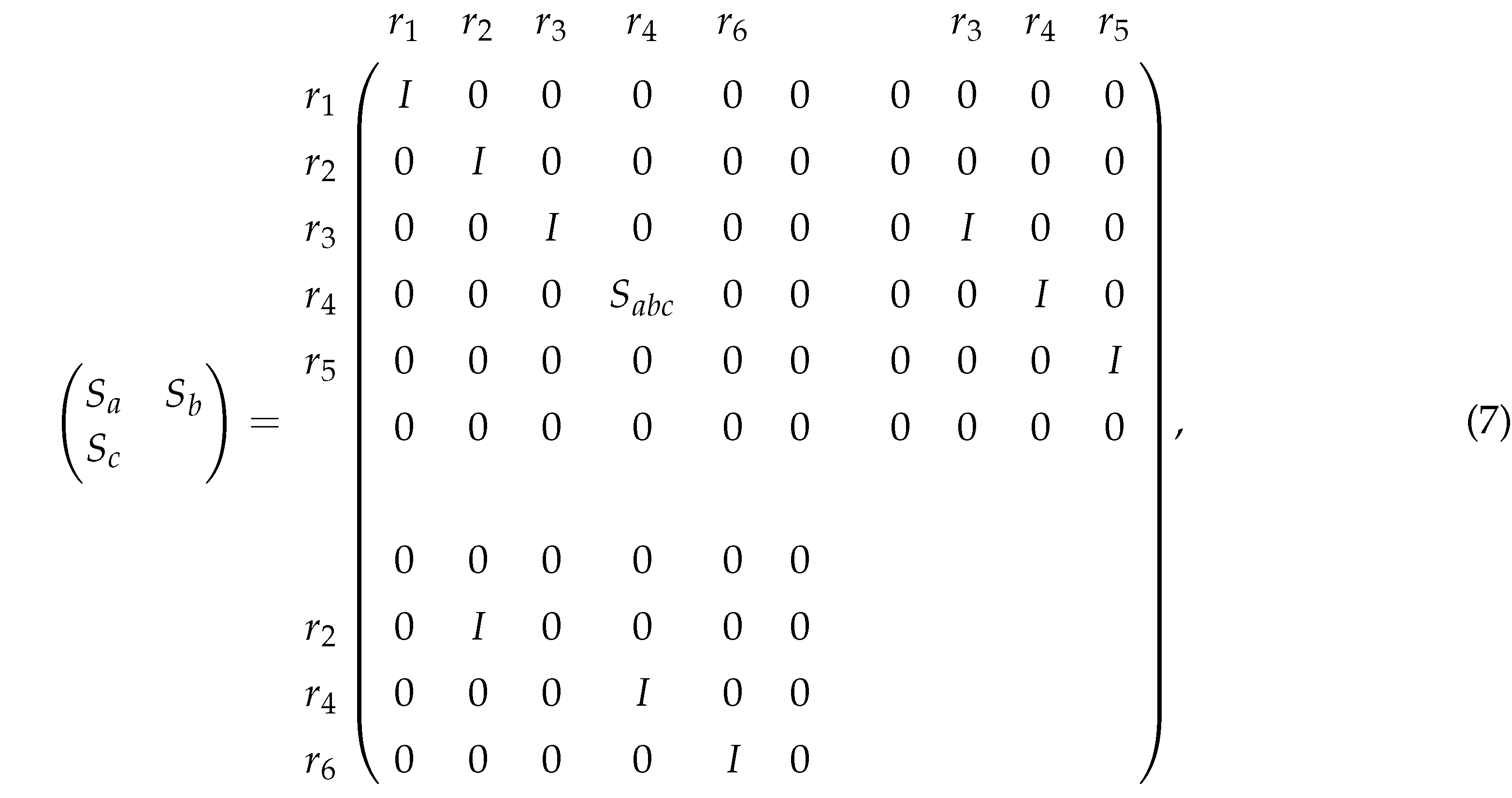
and

S_{a b c} = diag {σ_{1}, \dots, σ_{r_{4}}}

is square nonsingular diagonal with positive diagonal elements,

σ_{1}, \dots, σ_{r_{4}}

are defined to be the non-trivial restricted singular values of the matrix triplet

A, B, C

. Expressions for the integers

r_{1}, \dots, r_{6}

are the following:

\begin{matrix} r_{1} = r (\begin{matrix} A & B \\ C & 0 \end{matrix}) - r (B) - r (C), \end{matrix}

(8)

\begin{matrix} r_{2} = r (A, B) + r (C) - r (\begin{matrix} A & B \\ C & 0 \end{matrix}), \end{matrix}

(9)

\begin{matrix} r_{3} = r (B) + r (\begin{matrix} A \\ C \end{matrix}) - r (\begin{matrix} A & B \\ C & 0 \end{matrix}), \end{matrix}

(10)

\begin{matrix} r_{4} = r (A) + r (\begin{matrix} A & B \\ C & 0 \end{matrix}) - r (\begin{matrix} A \\ C \end{matrix}) - r (A, B), \end{matrix}

(11)

\begin{matrix} r_{5} = r (A, B) - r (A), r_{6} = r (\begin{matrix} A \\ C \end{matrix}) - r (A), \end{matrix}

(12)

where the symbol

r (A)

stands for the rank of the matrix A.

The following theorem presents the RSVD for three tensors under t-product.

Theorem 1

(T-RSVD). Let

A \in C^{m \times p \times n_{3}}, B \in C^{m \times q \times n_{3}},

and

C \in C^{t \times p \times n_{3}}

. Then

A, B,

and

C

can be factored as

\begin{matrix} A = P * S_{a} * Q, B = P * S_{b} * V, C = U * S_{c} * Q, \end{matrix}

(13)

where

U \in C^{t \times t \times n_{3}}

and

V \in C^{q \times q \times n_{3}}

are unitary,

P \in C^{m \times m \times n_{3}}, Q \in C^{p \times p \times n_{3}}

are invertible,

S_{a}

is a

m \times p \times n_{3}

f-diagonal tensor,

S_{b}

and

S_{c}

are

m \times q \times n_{3}

and

t \times p \times n_{3}

tensors whose frontal slices are, respectively, block lower-triangular and block upper-triangular matrices with the following forms

\begin{matrix} {(S_{b})}_{i} = \sum_{j = 1}^{n_{3}} ω^{(j - 1) (i - 1)} (\begin{matrix} 0 & 0 \\ 0 & I_{s_{j}} \\ 0 & 0 \end{matrix}), {(S_{c})}_{i} = \sum_{j = 1}^{n_{3}} ω^{(j - 1) (i - 1)} (\begin{matrix} 0 & 0 & 0 & 0 & 0 \\ 0 & I_{s_{j}^{'}} & 0 & 0 & 0 \\ 0 & 0 & 0 & I_{s_{j}^{''}} & 0 \end{matrix}), i = 1 \dots, n_{3} . \end{matrix}

Proof.

Let

\tilde{A} = bcirc (A) \in C^{(m n_{3}) \times (p n_{3})}, \tilde{B} = bcirc (B) \in C^{(m n_{3}) \times (q n_{3})},

and

\tilde{C} = bcirc (C) \in C^{(t n_{3}) \times (p n_{3})} .

It follows from (3) that

\begin{matrix} (F_{n_{3}} \otimes I_{m}) \tilde{A} (F_{n_{3}}^{*} \otimes I_{p}) = diag (\tilde{A_{1}}, \dots, \tilde{A_{n_{3}}}), \end{matrix}

\begin{matrix} (F_{n_{3}} \otimes I_{m}) \tilde{B} (F_{n_{3}}^{*} \otimes I_{q}) = diag (\tilde{B_{1}}, \dots, \tilde{B_{n_{3}}}), \end{matrix}

\begin{matrix} (F_{n_{3}} \otimes I_{t}) \tilde{C} (F_{n_{3}}^{*} \otimes I_{p}) = diag (\tilde{C_{1}}, \dots, \tilde{C_{n_{3}}}), \end{matrix}

where

F_{n_{3}}

n_{3} \times n_{3}

normalized DFT matrix,

\tilde{A_{i}}, \tilde{B_{i}},

and

\tilde{C_{i}}

are

m \times p, m \times q,

and

t \times p

matrices

i = 1, \dots, n_{3} .

Observe that

\tilde{A_{i}}

and

\tilde{B_{i}}

have the same number of columns, meanwhile

\tilde{A_{i}}

and

\tilde{C_{i}}

have the same number of rows. Applying RSVD (Lemma 1) to each matrix triplet

\tilde{A_{i}}, \tilde{B_{i}},

and

\tilde{C_{i}}

gives

\begin{matrix} (\begin{matrix} \tilde{A_{1}} \\ ⋱ \\ \tilde{A_{n_{3}}} \end{matrix}) = (\begin{matrix} P_{1} \\ ⋱ \\ P_{n_{3}} \end{matrix}) (\begin{matrix} Ω_{A_{1}} \\ ⋱ \\ Ω_{A_{n_{3}}} \end{matrix}) (\begin{matrix} Q_{1} \\ ⋱ \\ Q_{n_{3}} \end{matrix}), \end{matrix}

(14)

\begin{matrix} (\begin{matrix} \tilde{B_{1}} \\ ⋱ \\ \tilde{B_{n_{3}}} \end{matrix}) = (\begin{matrix} P_{1} \\ ⋱ \\ P_{n_{3}} \end{matrix}) (\begin{matrix} Ω_{B_{1}} \\ ⋱ \\ Ω_{B_{n_{3}}} \end{matrix}) (\begin{matrix} V_{1} \\ ⋱ \\ V_{n_{3}} \end{matrix}), \end{matrix}

(15)

and

\begin{matrix} (\begin{matrix} \tilde{C_{1}} \\ ⋱ \\ \tilde{C_{n_{3}}} \end{matrix}) = (\begin{matrix} U_{1} \\ ⋱ \\ U_{n_{3}} \end{matrix}) (\begin{matrix} Ω_{C_{1}} \\ ⋱ \\ Ω_{C_{n_{3}}} \end{matrix}) (\begin{matrix} Q_{1} \\ ⋱ \\ Q_{n_{3}} \end{matrix}), \end{matrix}

(16)

where the forms of

Ω_{A_{i}}, Ω_{B_{i}},

and

Ω_{C_{i}}

are given in (7),

U_{i}

and

V_{i}

are unitary, and

P_{i}

and

Q_{i}

are nonsingular. We multiply

(F_{n_{3}}^{*} \otimes I_{m}), (F_{n_{3}}^{*} \otimes I_{m}),

and

(F_{n_{3}}^{*} \otimes I_{t})

to the left of each of the block diagonal matrices in (14)–(16), respectively, and

(F_{n_{3}} \otimes I_{p}), (F_{n_{3}} \otimes I_{q}),

and

(F_{n_{3}} \otimes I_{p})

to the right of each of the block diagonal matrices in (14)–(16). Then, we obtain

\begin{matrix} bcirc (A) = & [(F_{n_{3}}^{*} \otimes I_{m}) (\begin{matrix} P_{1} \\ ⋱ \\ P_{n_{3}} \end{matrix}) (F_{n_{3}} \otimes I_{m})] \\ [(F_{n_{3}}^{*} \otimes I_{m}) (\begin{matrix} Ω_{A_{1}} \\ ⋱ \\ Ω_{A_{n_{3}}} \end{matrix}) (F_{n_{3}} \otimes I_{p})] \\ [(F_{n_{3}}^{*} \otimes I_{p}) (\begin{matrix} Q_{1} \\ ⋱ \\ Q_{n_{3}} \end{matrix}) (F_{n_{3}} \otimes I_{p})] \\ = & bcirc (P) bcirc (S_{a}) bcirc (Q), \end{matrix}

(17)

\begin{matrix} bcirc (B) = & [(F_{n_{3}}^{*} \otimes I_{m}) (\begin{matrix} P_{1} \\ ⋱ \\ P_{n_{3}} \end{matrix}) (F_{n_{3}} \otimes I_{m})] \\ [(F_{n_{3}}^{*} \otimes I_{m}) (\begin{matrix} Ω_{B_{1}} \\ ⋱ \\ Ω_{B_{n_{3}}} \end{matrix}) (F_{n_{3}} \otimes I_{q})] \\ [(F_{n_{3}}^{*} \otimes I_{q}) (\begin{matrix} V_{1} \\ ⋱ \\ V_{n_{3}} \end{matrix}) (F_{n_{3}} \otimes I_{q})] \\ = & bcirc (P) bcirc (S_{b}) bcirc (V), \end{matrix}

(18)

and

\begin{matrix} bcirc (C) = & [(F_{n_{3}}^{*} \otimes I_{t}) (\begin{matrix} U_{1} \\ ⋱ \\ U_{n_{3}} \end{matrix}) (F_{n_{3}} \otimes I_{t})] \\ [(F_{n_{3}}^{*} \otimes I_{t}) (\begin{matrix} Ω_{C_{1}} \\ ⋱ \\ Ω_{C_{n_{3}}} \end{matrix}) (F_{n_{3}} \otimes I_{p})] \\ [(F_{n_{3}}^{*} \otimes I_{p}) (\begin{matrix} Q_{1} \\ ⋱ \\ Q_{n_{3}} \end{matrix}) (F_{n_{3}} \otimes I_{p})] \\ = & bcirc (U) bcirc (S_{c}) bcirc (Q), \end{matrix}

(19)

which yields

A = P * S_{a} * Q,

(20)

B = P * S_{b} * V,

(21)

and

C = U * S_{c} * Q .

(22)

Note that

U

and

V

are unitary,

P

and

Q

are invertible. It follows from (4) that the frontal slices of

S_{a}, S_{b},

and

S_{c}

have the following forms

{(S_{a})}_{i} = \sum_{j = 1}^{n_{3}} ω^{(j - 1) (i - 1)} Ω_{A_{j}}, {(S_{b})}_{i} = \sum_{j = 1}^{n_{3}} ω^{(j - 1) (i - 1)} Ω_{B_{j}},

{(S_{c})}_{i} = \sum_{j = 1}^{n_{3}} ω^{(j - 1) (i - 1)} Ω_{C_{j}}, i = 1 \dots, n_{3} .

□

We provide the algorithm for T-RSVD.

Algorithm 1: Compute the T-RSVD of tensors $A, B,$ and $C$

Input:

A \in C^{m \times p \times n_{3}}, B \in C^{m \times q \times n_{3}}, C \in C^{t \times p \times n_{3}} .

Output:

S_{a} \in C^{m \times p \times n_{3}}, S_{b} \in C^{m \times q \times n_{3}}, S_{c} \in C^{t \times p \times n_{3}}, U \in C^{t \times t \times n_{3}}, V \in C^{q \times q \times n_{3}},

P \in C^{m \times m \times n_{3}}, Q \in C^{p \times p \times n_{3}} .

\tilde{A} = bcirc (A), \tilde{B} = bcirc (B), \tilde{C} = bcirc (C) .

(F_{n_{3}} \otimes I_{m}) \tilde{A} (F_{n_{3}}^{*} \otimes I_{p}) = diag (\tilde{A_{j}}), (F_{n_{3}} \otimes I_{m}) \tilde{B} (F_{n_{3}}^{*} \otimes I_{q}) = diag (\tilde{B_{j}}),

(F_{n_{3}} \otimes I_{t}) \tilde{C} (F_{n_{3}}^{*} \otimes I_{p}) = diag (\tilde{C_{j}}), j = 1, 2, \dots, n_{3} .

3. for

j = 1, \dots, n_{3}

% Give the RSVD of

\tilde{A_{j}}, \tilde{B_{j}},

and

\tilde{C_{j}}

by the method in [1],

\tilde{A_{j}} = P_{j} Ω_{A_{j}} Q_{j},

\tilde{B_{j}} = P_{j} Ω_{B_{j}} V_{j},

\tilde{C_{j}} = U_{j} Ω_{C_{j}} Q_{j},

end for

Ω_{A} = diag (Ω_{A_{j}}), Ω_{B} = diag (Ω_{B_{j}}), Ω_{C} = diag (Ω_{C_{j}}), U = diag (U_{j}), V = diag (V_{j}),

P = diag (P_{j}), Q = diag (Q_{j}) .

{\tilde{S}}_{a} = (F_{n_{3}}^{*} \otimes I_{m}) Ω_{A} (F_{n_{3}} \otimes I_{p}), {\tilde{S}}_{b} = (F_{n_{3}}^{*} \otimes I_{m}) Ω_{B} (F_{n_{3}} \otimes I_{q}), {\tilde{S}}_{c} = (F_{n_{3}}^{*} \otimes I_{t}) Ω_{C} (F_{n_{3}} \otimes I_{p}),

\tilde{U} = (F_{n_{3}}^{*} \otimes I_{t}) U (F_{n_{3}} \otimes I_{t}), \tilde{V} = (F_{n_{3}}^{*} \otimes I_{q}) V (F_{n_{3}} \otimes I_{q}),

\tilde{P} = (F_{n_{3}}^{*} \otimes I_{m}) P (F_{n_{3}} \otimes I_{m}), \tilde{Q} = (F_{n_{3}}^{*} \otimes I_{p}) Q (F_{n_{3}} \otimes I_{p}) .

S_{a} = {bcirc}^{- 1} ({\tilde{S}}_{a}), S_{b} = {bcirc}^{- 1} ({\tilde{S}}_{b}), S_{c} = {bcirc}^{- 1} ({\tilde{S}}_{c}),

U = {bcirc}^{- 1} (\tilde{U}), V = {bcirc}^{- 1} (\tilde{V}), P = {bcirc}^{- 1} (\tilde{P}), Q = {bcirc}^{- 1} (\tilde{Q}) .

The cost of Algorithm 1 is not less than

O ({(n_{1} \times n_{2} \times n_{3})}^{3})

Example 1.

Let

A \in C^{5 \times 4 \times 3}

B \in C^{5 \times 6 \times 3}

and

C \in C^{7 \times 4 \times 3}

be tensors with the following forms:

\begin{matrix} A_{1} = (\begin{matrix} \begin{matrix} 0.5303 + 0.5248 i & 0.4221 + 0.7424 i & 0.5356 + 0.7391 i & 0.6216 + 0.6644 i \\ 0.7312 + 1.0116 i & 0.1918 + 0.7801 i & 1.0096 + 0.6131 i & 0.6995 + 1.0930 i \\ 0.7828 + 0.9208 i & 0.5561 + 0.4061 i & 0.8372 + 0.1792 i & 0.8905 + 0.9073 i \\ 0.7793 + 0.9972 i & 1.2191 + 0.6961 i & 0.3713 + 0.5136 i & 1.1552 + 1.0565 i \\ 0.5657 + 0.2247 i & 0.4331 + 0.7622 i & 0.5833 + 0.8704 i & 0.6561 + 0.4125 i \end{matrix} \end{matrix}), \end{matrix}

\begin{matrix} A_{2} = (\begin{matrix} \begin{matrix} 0.7495 + 1.2373 i & 0.1073 + 0.3358 i & 1.0968 - 0.0209 i & 0.6810 + 1.1587 i \\ 0.4769 - 0.2104 i & 1.1669 + 0.9282 i & - 0.0650 + 1.2320 i & 0.8769 + 0.0870 i \\ 0.5336 + 0.7049 i & 0.0139 + 0.7114 i & 0.8243 + 0.6365 i & 0.4596 + 0.8100 i \\ 0.5427 + 1.2123 i & - 0.2579 + 0.5388 i & 1.0273 + 0.2411 i & 0.3576 + 1.1957 i \\ 0.5218 + 0.8433 i & 1.1630 + 0.5181 i & 0.0079 + 0.3463 i & 0.9135 + 0.8730 i \end{matrix} \end{matrix}), \end{matrix}

\begin{matrix} A_{3} = (\begin{matrix} \begin{matrix} 0.8390 + 0.3249 i & - 0.0225 + 0.4260 i & 1.3270 + 0.4157 i & 0.7047 + 0.4016 i \\ 0.6379 + 0.3782 i & 1.4253 + 0.5669 i & 0.0071 + 0.5724 i & 1.1182 + 0.4880 i \\ 0.8143 + 0.7469 i & 0.1163 + 0.2199 i & 1.1919 + 0.0088 i & 0.7398 + 0.7044 i \\ 0.7343 + 0.6969 i & 0.2639 + 0.6815 i & 0.9643 + 0.6020 i & 0.7312 + 0.7945 i \\ 0.2706 - 0.1724 i & 0.7472 + 0.8606 i & - 0.0959 + 1.1341 i & 0.5319 + 0.1001 i \end{matrix} \end{matrix}), \end{matrix}

\begin{matrix} B_{1} = (\begin{matrix} \begin{matrix} 0.9678 + 1.0857 i & 1.9658 + 2.4999 i & 1.8365 + 2.4539 i & 2.3199 + 2.7399 i & 1.8102 + 2.4752 i & 0.8597 + 1.3350 i & 1.2342 + 1.4315 i \\ 1.5437 + 1.4667 i & 2.7275 + 3.0925 i & 2.5159 + 2.8494 i & 2.7909 + 4.0341 i & 2.1110 + 3.0183 i & 0.4634 + 1.7009 i & 1.1811 + 2.3560 i \\ 1.4646 + 1.0428 i & 2.9047 + 2.0090 i & 2.7081 + 1.7155 i & 3.3544 + 3.0897 i & 2.6059 + 1.9291 i & 1.1449 + 1.1409 i & 1.7323 + 1.9562 i \\ 1.1014 + 1.3758 i & 2.8630 + 2.8554 i & 2.7241 + 2.5984 i & 4.0353 + 3.8373 i & 3.2509 + 2.7793 i & 2.3711 + 1.5791 i & 2.6126 + 2.2774 i \\ 1.0417 + 0.8922 i & 2.0977 + 2.2487 i & 1.9584 + 2.3345 i & 2.4568 + 2.0245 i & 1.9140 + 2.2563 i & 0.8852 + 1.1671 i & 1.2936 + 0.8882 i \end{matrix} \end{matrix}), \end{matrix}

\begin{matrix} B_{2} = (\begin{matrix} \begin{matrix} 1.6302 + 1.1994 i & 2.7995 + 2.1430 i & 2.5751 + 1.6989 i & 2.7673 + 3.7497 i & 2.0757 + 2.0271 i & 0.3098 + 1.2518 i & 1.0915 + 2.4986 i \\ 0.4485 + 0.7437 i & 1.7340 + 2.2485 i & 1.6849 + 2.5580 i & 2.9096 + 1.2503 i & 2.4047 + 2.3085 i & 2.2296 + 1.1078 i & 2.1604 + 0.1857 i \\ 1.1941 + 1.1835 i & 1.9959 + 2.6001 i & 1.8307 + 2.4705 i & 1.9049 + 3.1328 i & 1.4161 + 2.5553 i & 0.1049 + 1.4102 i & 0.6937 + 1.7458 i \\ 1.3604 + 1.3769 i & 2.0418 + 2.6560 i & 1.8506 + 2.2706 i & 1.6530 + 4.0758 i & 1.1719 + 2.5509 i & - 0.3966 + 1.5076 i & 0.3426 + 2.5781 i \\ 0.5517 + 1.0956 i & 1.9021 + 2.2274 i & 1.8386 + 1.9933 i & 3.0645 + 3.1096 i & 2.5188 + 2.1601 i & 2.2291 + 1.2407 i & 2.2119 + 1.8821 i \end{matrix} \end{matrix}), \end{matrix}

\begin{matrix} B_{3} = (\begin{matrix} \begin{matrix} 1.9015 + 0.6399 i & 3.1403 + 1.4586 i & 2.8768 + 1.4222 i & 2.9489 + 1.6319 i & 2.1830 + 1.4419 i & 0.0829 + 0.7815 i & 1.0316 + 0.8654 i \\ 0.6725 + 0.8131 i & 2.3250 + 1.8862 i & 2.2478 + 1.8607 i & 3.7500 + 2.0357 i & 3.0827 + 1.8697 i & 2.7315 + 1.0049 i & 2.7087 + 1.0514 i \\ 1.7713 + 0.7406 i & 3.0417 + 1.3392 i & 2.7979 + 1.0752 i & 3.0065 + 2.2965 i & 2.2550 + 1.2699 i & 0.3361 + 0.7787 i & 1.1856 + 1.5190 i \\ 1.5120 + 1.1491 i & 2.7359 + 2.5126 i & 2.5295 + 2.3793 i & 2.8771 + 3.0553 i & 2.1902 + 2.4674 i & 0.5972 + 1.3649 i & 1.2812 + 1.7124 i \\ 0.2089 + 0.7056 i & 0.9802 + 2.1076 i & 0.9596 + 2.3849 i & 1.7398 + 1.2161 i & 1.4483 + 2.1608 i & 1.4224 + 1.0417 i & 1.3392 + 0.2141 i \end{matrix} \end{matrix}), \end{matrix}

\begin{matrix} C_{1} = (\begin{matrix} \begin{matrix} 7.1881 + 6.9753 i & 5.1342 + 6.9579 i & 7.6688 + 6.1966 i & 8.1884 + 7.9916 i \\ 4.8046 + 4.6507 i & 2.4018 + 4.0024 i & 5.8412 + 3.3377 i & 5.0574 + 5.1448 i \\ 6.5231 + 6.3144 i & 4.6489 + 5.9511 i & 6.9664 + 5.1761 i & 7.4267 + 7.1342 i \\ 5.0711 + 4.5700 i & 5.6075 + 5.0339 i & 4.0314 + 4.6524 i & 6.5785 + 5.3729 i \\ 5.6683 + 6.0800 i & 3.7989 + 5.4458 i & 6.2208 + 4.6295 i & 6.3563 + 6.7875 i \\ 3.9585 + 3.9067 i & 3.1749 + 4.4012 i & 3.9818 + 4.0993 i & 4.6496 + 4.6212 i \end{matrix} \end{matrix}), \end{matrix}

\begin{matrix} C_{2} = (\begin{matrix} \begin{matrix} 4.8070 + 4.3309 i & 4.0376 + 4.7113 i & 4.7088 + 4.3351 i & 5.7199 + 5.0747 i \\ 4.7909 + 3.8380 i & 3.6841 + 4.9274 i & 4.9292 + 4.7796 i & 5.5635 + 4.7139 i \\ 5.0686 + 4.9549 i & 2.5796 + 4.3957 i & 6.1302 + 3.7199 i & 5.3538 + 5.5192 i \\ 6.0918 + 6.4247 i & 4.4663 + 5.7944 i & 6.4191 + 4.9416 i & 6.9861 + 7.1838 i \\ 4.6481 + 4.4668 i & 2.9568 + 3.9805 i & 5.2112 + 3.3757 i & 5.1483 + 4.9807 i \\ 5.6523 + 5.9783 i & 3.4304 + 4.8733 i & 6.4517 + 3.9518 i & 6.1939 + 6.5352 i \end{matrix} \end{matrix}), \end{matrix}

\begin{matrix} C_{3} = (\begin{matrix} \begin{matrix} 5.8659 + 5.3457 i & 4.4210 + 6.0571 i & 6.0977 + 5.6524 i & 6.7756 + 6.3334 i \\ 5.4631 + 5.1432 i & 2.8010 + 5.0694 i & 6.5931 + 4.4929 i & 5.7788 + 5.8750 i \\ 7.2234 + 7.1743 i & 6.2645 + 7.0710 i & 6.9389 + 6.2668 i & 8.6748 + 8.1950 i \\ 5.5242 + 5.4475 i & 6.0286 + 5.3725 i & 4.4471 + 4.7627 i & 7.1340 + 6.2235 i \\ 4.8612 + 5.0317 i & 2.0329 + 3.6799 i & 6.1858 + 2.8003 i & 4.9566 + 5.3788 i \\ 5.3460 + 5.1352 i & 4.7360 + 5.8883 i & 5.0663 + 5.5168 i & 6.4605 + 6.1042 i \end{matrix} \end{matrix}) . \end{matrix}

It follows from Theorem 1 and Algorithm 1 that

\begin{matrix} A = P * S_{a} * Q, B = P * S_{b} * V, C = U * S_{c} * Q, \end{matrix}

(23)

where

U \in C^{t \times t \times n_{3}}

and

V \in C^{q \times q \times n_{3}}

are unitary,

P \in C^{m \times m \times n_{3}}, Q \in C^{p \times p \times n_{3}}

are invertible, and

\begin{matrix} P_{1} = (\begin{matrix} \begin{matrix} 0.6408 - 0.5877 i & - 0.0936 - 0.0107 i & - 0.4060 + 0.5214 i & 2.2421 + 5.0044 i & 0.2949 + 0.0390 i \\ - 0.1613 + 0.2793 i & 0.4269 - 0.0810 i & 0.4228 - 1.2971 i & 2.6692 + 5.3346 i & 0.3346 + 0.0419 i \\ 0.4351 - 0.4090 i & - 0.6897 + 0.1941 i & - 0.7972 + 0.1545 i & 2.3592 + 5.8345 i & - 0.6301 - 0.0906 i \\ 0.4874 - 0.7717 i & - 0.9595 + 0.3726 i & - 0.2353 + 1.3777 i & 2.0832 + 8.1176 i & 0.1698 + 0.0205 i \\ 0.1609 - 0.1738 i & 0.8428 - 0.1838 i & 0.9707 - 0.3759 i & 1.4278 + 6.5459 i & - 0.4527 - 0.0595 i \end{matrix} \end{matrix}), \end{matrix}

\begin{matrix} P_{2} = (\begin{matrix} \begin{matrix} - 0.2512 + 0.3184 i & - 0.8487 + 0.5414 i & - 1.1722 - 1.0526 i & 3.0836 + 7.1109 i & - 0.1229 - 0.0429 i \\ - 0.3248 + 0.4861 i & 1.0281 - 0.4627 i & 1.7064 + 1.6331 i & 5.3474 + 7.9779 i & - 0.0898 - 0.0413 i \\ - 0.2539 + 0.3055 i & - 0.0275 - 0.3210 i & - 0.4593 - 0.2713 i & 3.7814 + 5.1409 i & - 0.0982 + 0.0136 i \\ - 0.3560 + 0.0728 i & - 0.4230 - 0.1031 i & - 0.7313 - 1.1984 i & 4.1175 + 6.0276 i & - 0.0816 - 0.0287 i \\ 0.3311 - 0.3674 i & - 0.4491 + 0.6748 i & 0.5431 + 0.8102 i & 2.2330 + 5.9796 i & - 0.0161 + 0.0261 i \end{matrix} \end{matrix}), \end{matrix}

\begin{matrix} P_{3} = (\begin{matrix} \begin{matrix} - 0.3059 + 0.3610 i & 0.5091 - 0.4685 i & - 0.5184 - 0.9038 i & 4.2031 + 6.9941 i & 0.1701 + 0.0145 i \\ 0.6811 - 0.5568 i & - 0.3334 + 0.5769 i & 0.9122 + 1.3152 i & 2.8736 + 7.2549 i & 0.1871 + 0.0129 i \\ - 0.1097 + 0.1755 i & - 0.3939 + 0.0771 i & - 0.8263 - 0.9132 i & 3.7283 + 8.3036 i & 0.1302 + 0.0584 i \\ - 0.5188 + 0.2754 i & 0.1895 - 0.4533 i & - 0.0753 - 0.1377 i & 2.3868 + 9.6501 i & 0.1436 + 0.0154 i \\ - 0.5290 + 0.5041 i & 0.9653 - 0.4482 i & 1.4892 + 1.1565 i & 3.9351 + 5.1095 i & - 0.0641 + 0.0167 i \end{matrix} \end{matrix}), \end{matrix}

\begin{matrix} Q_{1} = (\begin{matrix} \begin{matrix} - 0.0152 + 0.0008 i & 0.0052 - 0.0003 i & 0.0042 - 0.0002 i & 0.0085 - 0.0004 i \\ 0.3822 - 0.8686 i & - 0.5113 + 0.7359 i & 0.0025 + 0.6981 i & 0.1330 - 0.5357 i \\ - 1.3744 + 0.1132 i & 2.2744 - 2.3223 i & - 0.5762 + 3.5012 i & - 0.3227 - 0.8922 i \\ 16.3877 - 9.0211 i & 15.0754 - 5.6503 i & 14.7485 - 9.8723 i & 18.7357 - 10.3581 i \end{matrix} \end{matrix}), \end{matrix}

\begin{matrix} Q_{2} = (\begin{matrix} \begin{matrix} - 0.0159 + 0.0167 i & 0.0055 - 0.0058 i & 0.0044 - 0.0047 i & 0.0089 - 0.0093 i \\ - 0.1900 - 0.4386 i & 0.2039 + 0.4691 i & 0.0773 + 0.1913 i & - 0.0979 - 0.2206 i \\ - 0.0433 - 0.1733 i & 0.7916 + 0.1304 i & - 1.0174 + 0.1131 i & 0.2912 - 0.1051 i \\ 17.1512 - 7.2539 i & 15.0898 - 4.4501 i & 16.2790 - 8.6406 i & 19.4136 - 8.4856 i \end{matrix} \end{matrix}), \end{matrix}

\begin{matrix} Q_{3} = (\begin{matrix} \begin{matrix} - 0.0155 - 0.0167 i & 0.0054 + 0.0058 i & 0.0043 + 0.0047 i & 0.0087 + 0.0093 i \\ - 0.2820 - 0.3994 i & 0.2413 + 0.4149 i & 0.2093 + 0.1722 i & - 0.1650 - 0.1771 i \\ 0.4003 + 0.0073 i & 0.4382 + 0.0189 i & - 1.5852 + 0.0118 i & 0.5705 + 0.0154 i \\ 19.0878 - 3.7427 i & 17.2905 - 0.7168 i & 17.6647 - 5.5544 i & 22.0257 - 4.3068 i \end{matrix} \end{matrix}), \end{matrix}

\begin{matrix} U_{1} = (\begin{matrix} \begin{matrix} 0.1054 + 0.2152 i & 0.0949 - 0.0731 i & 0.0209 - 0.0258 i & 0.2220 + 0.0214 i & 0.0051 - 0.1728 i & - 0.0446 + 0.1700 i \\ - 0.1830 - 0.0106 i & 0.3933 - 0.2579 i & 0.0145 + 0.1753 i & - 0.0275 + 0.1724 i & - 0.1577 - 0.2441 i & 0.1679 + 0.0948 i \\ - 0.1066 - 0.1453 i & - 0.0150 + 0.0924 i & - 0.0448 + 0.0555 i & - 0.0960 + 0.0102 i & - 0.0641 - 0.1135 i & 0.2924 + 0.0744 i \\ 0.1422 + 0.0776 i & 0.1950 - 0.1345 i & 0.2179 - 0.0819 i & - 0.1872 + 0.0065 i & 0.2229 + 0.3532 i & 0.1096 + 0.1109 i \\ 0.3893 + 0.1686 i & 0.0423 + 0.0307 i & - 0.0311 - 0.0038 i & - 0.1386 - 0.0652 i & - 0.1125 + 0.0171 i & - 0.1152 + 0.1255 i \\ - 0.1001 + 0.0303 i & 0.3373 - 0.1433 i & - 0.1972 - 0.1863 i & 0.0041 + 0.0017 i & 0.0424 + 0.0948 i & 0.2399 + 0.0643 i \end{matrix} \end{matrix}), \end{matrix}

\begin{matrix} U_{2} = (\begin{matrix} \begin{matrix} - 0.0271 + 0.0574 i & - 0.4738 + 0.1835 i & 0.1470 - 0.1615 i & - 0.0016 + 0.0967 i & 0.0458 + 0.0943 i & 0.4059 + 0.0489 i \\ - 0.1138 + 0.0479 i & 0.2263 - 0.0749 i & 0.0146 + 0.1956 i & 0.3062 - 0.1033 i & 0.0124 + 0.1959 i & - 0.0104 + 0.1229 i \\ 0.0058 - 0.1376 i & - 0.1306 + 0.0788 i & 0.0147 + 0.0614 i & 0.1488 - 0.1841 i & - 0.0683 - 0.1907 i & 0.2169 + 0.0885 i \\ - 0.3325 - 0.0111 i & - 0.0530 - 0.0575 i & 0.0370 + 0.1065 i & 0.1376 - 0.1857 i & 0.1034 - 0.1806 i & - 0.0858 + 0.1292 i \\ - 0.0897 + 0.0322 i & - 0.2217 - 0.0040 i & - 0.2887 + 0.2487 i & - 0.2355 + 0.0075 i & - 0.1306 - 0.0206 i & 0.2770 + 0.0877 i \\ 0.0872 - 0.0300 i & - 0.0489 + 0.0535 i & - 0.3116 - 0.0649 i & - 0.1771 + 0.2345 i & - 0.0770 - 0.2311 i & - 0.1628 + 0.2071 i \end{matrix} \end{matrix}), \end{matrix}

\begin{matrix} U_{3} = (\begin{matrix} \begin{matrix} 0.2309 + 0.0505 i & - 0.1479 + 0.1096 i & - 0.1576 + 0.2048 i & 0.2842 - 0.0579 i & 0.0791 + 0.0871 i & - 0.1743 + 0.1854 i \\ 0.2495 - 0.1127 i & - 0.1168 + 0.1075 i & 0.2459 - 0.0555 i & 0.1508 + 0.0639 i & - 0.1420 - 0.2668 i & - 0.0037 + 0.1078 i \\ - 0.4449 - 0.2074 i & - 0.2231 + 0.0297 i & 0.1255 - 0.0258 i & - 0.2640 + 0.1617 i & 0.0398 + 0.2650 i & - 0.3123 + 0.2548 i \\ 0.2953 + 0.0149 i & 0.1418 + 0.0568 i & - 0.0295 + 0.1790 i & - 0.2309 + 0.0448 i & 0.2169 + 0.2944 i & 0.1615 + 0.1433 i \\ 0.0385 + 0.1177 i & 0.1669 - 0.0418 i & 0.2708 - 0.3069 i & - 0.2373 + 0.0416 i & - 0.2154 - 0.2440 i & - 0.0079 + 0.1162 i \\ - 0.0826 - 0.1074 i & - 0.0056 - 0.0327 i & - 0.0647 - 0.3652 i & 0.3285 - 0.2423 i & 0.1011 + 0.1815 i & 0.0755 + 0.0775 i \end{matrix} \end{matrix}), \end{matrix}

\begin{matrix} V_{1} = (\begin{matrix} \begin{matrix} - 0.3415 + 0.1010 i & 0.0300 - 0.2416 i & 0.1807 + 0.1893 i & 0.0558 - 0.1649 i & - 0.0886 + 0.1240 i & - 0.1395 - 0.1271 i & 0.0734 + 0.2405 i \\ 0.2890 + 0.0317 i & - 0.3653 - 0.0220 i & - 0.0635 - 0.1062 i & 0.1117 + 0.1213 i & 0.2928 + 0.0604 i & - 0.0117 + 0.0348 i & - 0.1816 - 0.1726 i \\ 0.0874 + 0.2393 i & 0.2122 - 0.0524 i & 0.0238 - 0.0688 i & 0.0848 - 0.0480 i & - 0.4611 + 0.0309 i & 0.3490 + 0.0988 i & - 0.1682 - 0.0256 i \\ 0.3112 - 0.2922 i & - 0.0508 - 0.0055 i & 0.2356 + 0.2536 i & - 0.3086 + 0.0646 i & - 0.2476 - 0.1863 i & 0.1613 - 0.0736 i & 0.3172 + 0.0636 i \\ 0.1966 - 0.1029 i & 0.0407 + 0.1393 i & - 0.0874 + 0.3287 i & 0.2014 - 0.4036 i & - 0.1963 + 0.2617 i & - 0.3328 + 0.1715 i & 0.0904 - 0.3965 i \\ - 0.1763 + 0.3055 i & - 0.0640 + 0.3116 i & 0.0264 + 0.2972 i & - 0.1110 - 0.1227 i & 0.1530 - 0.0536 i & 0.3092 - 0.5074 i & - 0.0026 - 0.3738 i \\ 0.0089 - 0.1151 i & 0.0295 - 0.2376 i & 0.0286 - 0.2216 i & 0.0459 - 0.2883 i & 0.0381 - 0.2235 i & 0.0328 - 0.1129 i & 0.0325 - 0.1580 i \end{matrix} \end{matrix}), \end{matrix}

\begin{matrix} V_{2} = (\begin{matrix} \begin{matrix} - 0.1297 - 0.1675 i & 0.1617 - 0.0854 i & - 0.0165 + 0.0411 i & - 0.1585 + 0.1909 i & 0.0221 + 0.0319 i & - 0.1052 - 0.0653 i & 0.2073 - 0.1539 i \\ - 0.1460 - 0.0398 i & 0.3177 + 0.0404 i & - 0.2142 - 0.0586 i & - 0.1842 - 0.1175 i & 0.1187 + 0.1507 i & - 0.1224 - 0.1249 i & 0.1848 + 0.1410 i \\ 0.2523 + 0.0383 i & 0.1733 - 0.0432 i & - 0.1905 - 0.0448 i & - 0.0875 + 0.1668 i & - 0.0881 - 0.0385 i & 0.2080 + 0.0938 i & - 0.0417 - 0.2169 i \\ - 0.0506 + 0.1462 i & 0.0356 - 0.1132 i & - 0.1192 - 0.0120 i & 0.0142 - 0.0373 i & 0.1457 + 0.0954 i & - 0.0786 + 0.0005 i & - 0.0253 + 0.0135 i \\ - 0.0858 - 0.0843 i & - 0.0128 - 0.0194 i & 0.0478 + 0.0345 i & - 0.1027 - 0.0854 i & 0.0893 + 0.0816 i & 0.1421 + 0.1412 i & - 0.0558 - 0.0372 i \\ - 0.0696 - 0.0422 i & - 0.0683 - 0.0288 i & - 0.0686 - 0.0144 i & 0.0534 - 0.0184 i & 0.0216 + 0.0195 i & 0.1322 + 0.0649 i & 0.1099 + 0.0117 i \\ 0.0581 - 0.0545 i & 0.1136 - 0.1148 i & 0.1071 - 0.1088 i & 0.1218 - 0.1328 i & 0.0985 - 0.1081 i & 0.0376 - 0.0536 i & 0.0579 - 0.0704 i \end{matrix} \end{matrix}), \end{matrix}

\begin{matrix} V_{3} = (\begin{matrix} \begin{matrix} - 0.1006 + 0.1861 i & 0.4325 + 0.0891 i & - 0.2664 - 0.1355 i & - 0.0683 - 0.0691 i & - 0.0932 - 0.0146 i & 0.0766 + 0.1185 i & - 0.0017 - 0.0174 i \\ - 0.0680 - 0.1072 i & 0.1545 + 0.0189 i & - 0.3050 + 0.0072 i & - 0.0057 + 0.0969 i & 0.2728 - 0.0343 i & - 0.1181 - 0.0068 i & - 0.0462 - 0.0838 i \\ 0.0460 - 0.1893 i & 0.0507 - 0.0294 i & - 0.2515 + 0.1265 i & 0.0121 - 0.0096 i & 0.2423 + 0.0099 i & - 0.0580 - 0.1324 i & - 0.0801 + 0.1028 i \\ 0.1875 - 0.0357 i & 0.0615 + 0.1229 i & - 0.0588 - 0.0883 i & - 0.3116 + 0.0288 i & 0.1080 - 0.0421 i & - 0.0381 + 0.0434 i & 0.2962 - 0.0591 i \\ - 0.0765 - 0.0494 i & 0.0254 - 0.0175 i & 0.1073 + 0.0083 i & - 0.1587 - 0.0325 i & 0.1164 + 0.0431 i & 0.1268 + 0.0862 i & - 0.1286 - 0.0023 i \\ - 0.0533 - 0.0247 i & - 0.1041 - 0.0263 i & - 0.1371 - 0.0283 i & 0.1006 + 0.0248 i & - 0.0428 + 0.0062 i & 0.0822 + 0.0482 i & 0.1601 + 0.0455 i \\ 0.1279 + 0.0821 i & 0.2705 + 0.1885 i & 0.2540 + 0.1794 i & 0.3278 + 0.2372 i & 0.2590 + 0.1932 i & 0.1360 + 0.1169 i & 0.1811 + 0.1386 i \end{matrix} \end{matrix}), \end{matrix}

\begin{matrix} {(S_{a})}_{1} = (\begin{matrix} \begin{matrix} 1 & 0 & 0 & 0 \\ 0 & 0.4583 & 0 & 0 \\ 0 & 0 & 0.1069 & 0 \\ 0 & 0 & 0 & 0.0161 \\ 0 & 0 & 0 & 0 \end{matrix} \end{matrix}), \end{matrix}

\begin{matrix} {(S_{a})}_{2} = (\begin{matrix} \begin{matrix} 0 & 0 & 0 & 0 \\ 0 & - 0.0940 - 0.0121 i & 0 & 0 \\ 0 & 0 & - 0.0106 + 0.0028 i & 0 \\ 0 & 0 & 0 & - 0.0070 + 0.0002 i \\ 0 & 0 & 0 & 0 \end{matrix} \end{matrix}), \end{matrix}

\begin{matrix} {(S_{a})}_{3} = (\begin{matrix} \begin{matrix} 0 & 0 & 0 & 0 \\ 0 & - 0.0940 + 0.0121 i & 0 & 0 \\ 0 & 0 & - 0.0106 - 0.0028 i & 0 \\ 0 & 0 & 0 & - 0.0070 - 0.0002 i \\ 0 & 0 & 0 & 0 \end{matrix} \end{matrix}), \end{matrix}

\begin{matrix} {(S_{b})}_{1} = (\begin{matrix} \begin{matrix} 0 & 0 & 0 & 0 & 0 & 0 & 0 \\ 0 & 0 & 0 & 0 & 1 & 0 & 0 \\ 0 & 0 & 0 & 0 & 0 & 1 & 0 \\ 0 & 0 & 0 & 0 & 0 & 0 & 1 \\ 0 & 0 & 0 & 0 & 0 & 0 & 0 \end{matrix} \end{matrix}), {(S_{b})}_{2} = (\begin{matrix} \begin{matrix} 0 & 0 & 0 & 0 & 0 & 0 & 0 \\ 0 & 0 & 0 & 0 & 0 & 0 & 0 \\ 0 & 0 & 0 & 0 & 0 & 0 & 0 \\ 0 & 0 & 0 & 0 & 0 & 0 & 0 \\ 0 & 0 & 0 & 0 & 0 & 0 & 0 \end{matrix} \end{matrix}), {(S_{b})}_{3} = (\begin{matrix} \begin{matrix} 0 & 0 & 0 & 0 & 0 & 0 & 0 \\ 0 & 0 & 0 & 0 & 0 & 0 & 0 \\ 0 & 0 & 0 & 0 & 0 & 0 & 0 \\ 0 & 0 & 0 & 0 & 0 & 0 & 0 \\ 0 & 0 & 0 & 0 & 0 & 0 & 0 \end{matrix} \end{matrix}), \end{matrix}

\begin{matrix} {(S_{c})}_{1} = (\begin{matrix} \begin{matrix} 0 & 0 & 0 & 0 \\ 0 & 0 & 0 & 0 \\ 1 & 0 & 0 & 0 \\ 0 & 1 & 0 & 0 \\ 0 & 0 & 1 & 0 \\ 0 & 0 & 0 & 1 \end{matrix} \end{matrix}), {(S_{c})}_{2} = (\begin{matrix} \begin{matrix} 0 & 0 & 0 & 0 \\ 0 & 0 & 0 & 0 \\ 0 & 0 & 0 & 0 \\ 0 & 0 & 0 & 0 \\ 0 & 0 & 0 & 0 \\ 0 & 0 & 0 & 0 \end{matrix} \end{matrix}), {(S_{c})}_{3} = (\begin{matrix} \begin{matrix} 0 & 0 & 0 & 0 \\ 0 & 0 & 0 & 0 \\ 0 & 0 & 0 & 0 \\ 0 & 0 & 0 & 0 \\ 0 & 0 & 0 & 0 \\ 0 & 0 & 0 & 0 \end{matrix} \end{matrix}) . \end{matrix}

As special cases of T-RSVD, we obtain T-PSVD and T-QSVD for two tensors.

Corollary 1

(T-PSVD [8]). Let

A \in C^{m \times n_{2} \times n_{3}}

and

B \in C^{h \times n_{2} \times n_{3}}

. Then

A

and

B

can be factored as

\begin{matrix} A = U * S_{a} * P, B = V * S_{b} * P^{- *}, \end{matrix}

where

U \in C^{m \times m \times n_{3}}

and

V \in C^{h \times h \times n_{3}}

are unitary, and

P \in C^{n_{2} \times n_{2} \times n_{3}}

is invertible,

S_{a}

is a

m \times n_{2} \times n_{3}

f-diagonal tensor,

S_{b}

is a

h \times n_{2} \times n_{3}

tensor whose frontal slices have the following form

\begin{matrix} {(S_{b})}_{i} = \sum_{j = 1}^{n_{3}} ω^{(j - 1) (i - 1)} (\begin{matrix} S_{r_{1 j}} & 0 & 0 & 0 \\ 0 & 0 & I_{r_{3 j}} & 0 \\ 0 & 0 & 0 & 0 \end{matrix}), i = 1, \dots, n_{3} . \end{matrix}

Corollary 2

(T-QSVD [8]). Let

A \in C^{m \times n_{2} \times n_{3}}

and

B \in C^{h \times n_{2} \times n_{3}}

. Then

A

and

B

can be factored as

\begin{matrix} A = U * S_{a} * P, B = V * S_{b} * P, \end{matrix}

where

U \in C^{m \times m \times n_{3}}

and

V \in C^{h \times h \times n_{3}}

are unitary,

P \in C^{n_{2} \times n_{2} \times n_{3}}

is invertible,

S_{a}

is a

m \times n_{2} \times n_{3}

f-diagonal tensor,

S_{b}

is a

h \times n_{2} \times n_{3}

tensor whose frontal slices have the following forms

\begin{matrix} {(S_{b})}_{i} = \sum_{j = 1}^{n_{3}} ω^{(j - 1) (i - 1)} (\begin{matrix} 0 & 0 & 0 \\ 0 & I_{r_{j}} & 0 \end{matrix}), i = 1 \dots, n_{3} . \end{matrix}

4. An application from color image watermarking processing

In this section, we use a third-order tensor

A \in C^{m \times n \times 3}

stand for color image, where the number “3” represents the three channels of RGB, and m and n denote hight and width of the image. Then we present the T-RSVD-based color image watermarking schemes. At present, the research on the algorithm of adding a gray or color watermark to a color image is very rich. Moreover, B. Harjito et al. proposed the method to add two gray watermarks to a gray image [7]. However, to our knowledge, there has been little work on adding three color watermarks to one color image. Based on T-RSVD, we implant three color watermarks into a color image at the same time, and only save two keys to ensure extraction process.

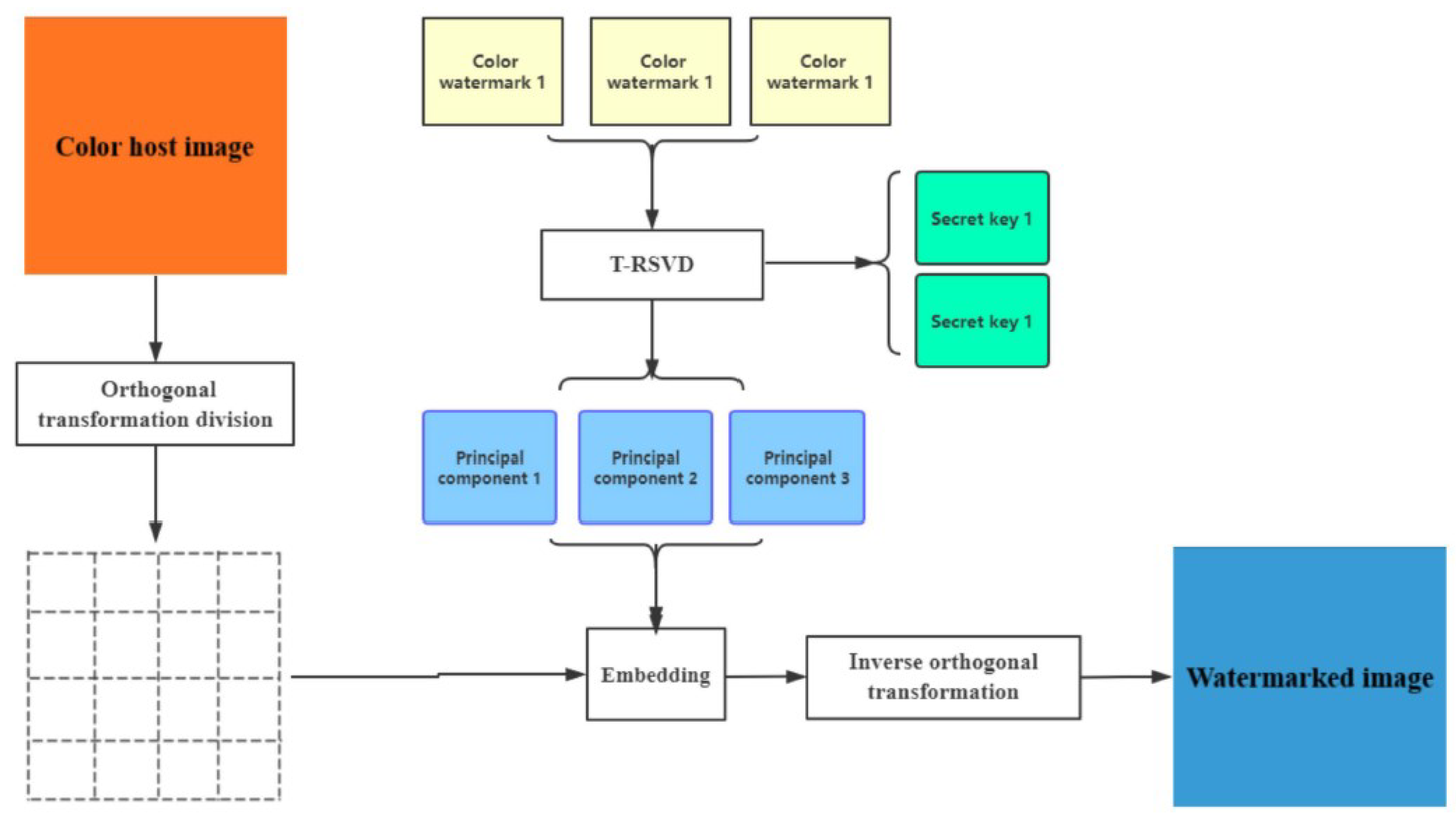
Let

F

be a color host image of size

M \times M \times 3

. Three color watermark images of the same size

N \times N \times 3

, i.e.,

A

B

and

C

, are simultaneously inserted into the color host image. The formal procedures of the T-RSVD-based color watermark embedding are given as follows.

A1.: T-RSVD-based decomposes three color watermark images $A$ , $B$ and $C$ ,

$A = P * S_{a} * Q,$

$B = P * S_{b} * V,$

$C = U * S_{c} * Q,$

where $P$ and $U$ are the secret keys and saved to extract the implanted watermarks.
A2.: Calculate the main components of each color watermark image,

$A_{w} \Leftarrow S_{a} * Q, B_{w} \Leftarrow S_{b} * V, C_{w} \Leftarrow S_{c} * Q .$
A3.: Orthogonal transformation divides the color host image $F$ into several non-overlapping color image blocks of size $N \times N \times 3$ , and $T_{i j} \in C^{N \times N \times 3}$ is the orthogonal transformed image on block position $(i, j)$ , $i, j = 1, \dots, m$ , where $m = \frac{M}{N}$ .
A4.: Implant the main components $A_{w}$ , $B_{w}$ and $C_{w}$ into the transformed color host image blocks $T_{11}$ , $T_{21}$ and $T_{12}$ :

$T_{11} \Leftarrow T_{11} + α A_{w},$

$T_{21} \Leftarrow T_{21} + α B_{w} .$

$T_{12} \Leftarrow T_{12} + α C_{w},$

where $α$ is a scale factor used to control watermarking strength [7]. When the value of $α$ is actually confirmed, the larger $α$ is, the stronger the robustness of watermark is, and the weaker the invisibility of the watermark is. The balance between robustness and invisibility needs to be considered. Save $T_{11}$ , $T_{21}$ and $T_{12}$ to guarantee the extraction.
A5.: Implement inverse orthogonal transformation for all image blocks $T_{i j}$ , and gain the watermarked color image $F_{w}$ .

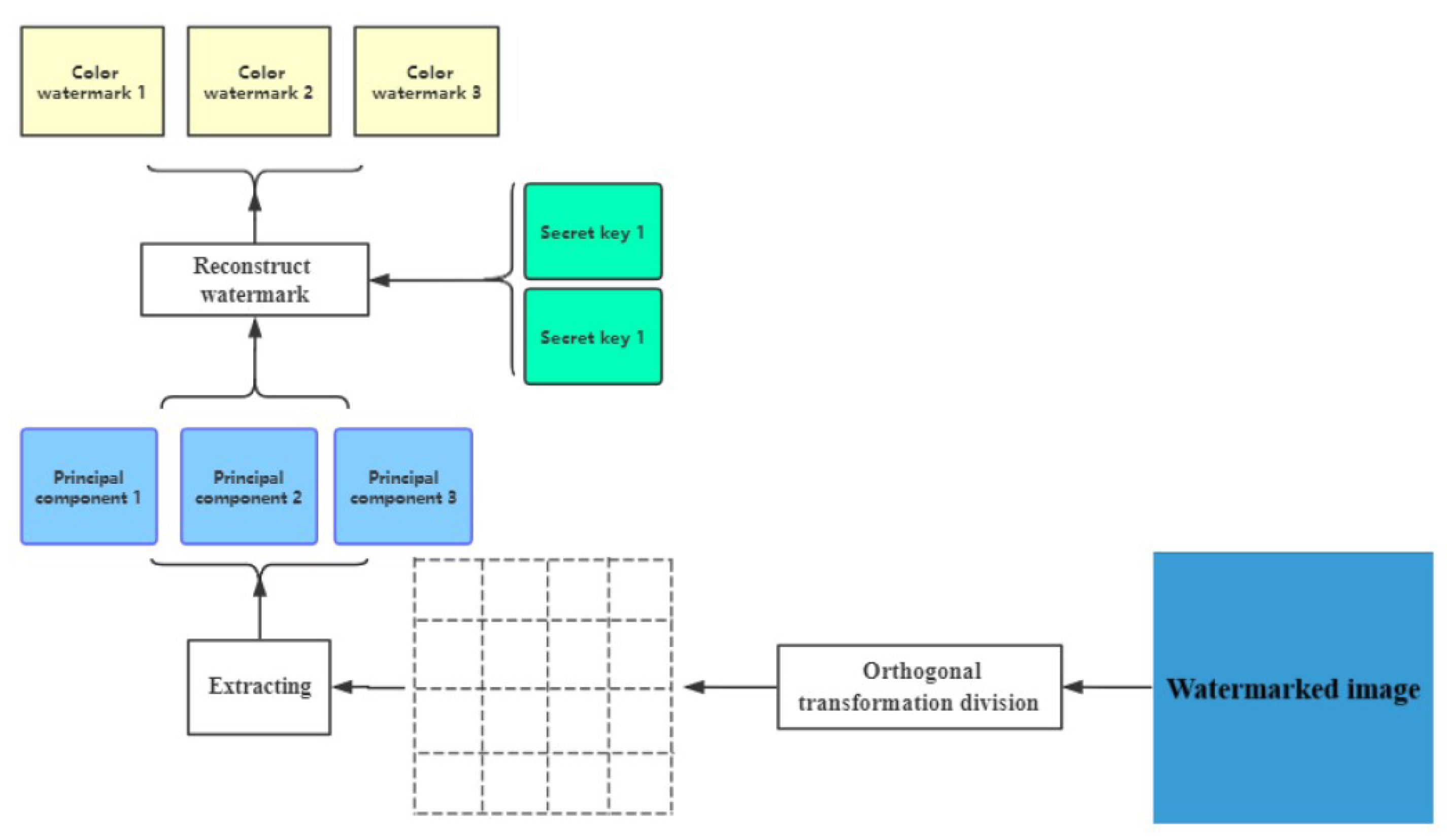
The formal procedure of the T-RSVD-based color watermark extraction process is given as follows:

B1.: Split the watermarked color image $F_{w}$ into several non-overlapping color image blocks ${\hat{T}}_{i j}$ with size $N \times N \times 3$ , $i, j = 1, \dots, m$ .
B2.: Extract the main components of each color watermark image as follows:

${\hat{A}}_{w} \Leftarrow \frac{1}{α} ({\hat{T}}_{11} - T_{11}),$

${\hat{B}}_{w} \Leftarrow \frac{1}{α} ({\hat{T}}_{21} - T_{21}),$

${\hat{C}}_{w} \Leftarrow \frac{1}{α} ({\hat{T}}_{12} - T_{12}) .$
B3.: Calculate the extracted watermarks $\hat{A}$ , $\hat{B}$ , and $\hat{C}$ :

$\hat{A} \Leftarrow P * {\hat{A}}_{w},$

$\hat{B} \Leftarrow P * {\hat{B}}_{w},$

$\hat{C} \Leftarrow U * {\hat{C}}_{w} .$

The imperceptibility of the proposed schemes can be measured by Peak-Signalto-Noise-Ratio (PSNR) [7], when the value of PSNR is greater than 30, the signal distortion is less. Now, we present the basic framework for implanting three color watermarks concurrently into a color image, as well as a frame diagram for the extraction of the color watermarked image in Figure 1 and Figure 2.

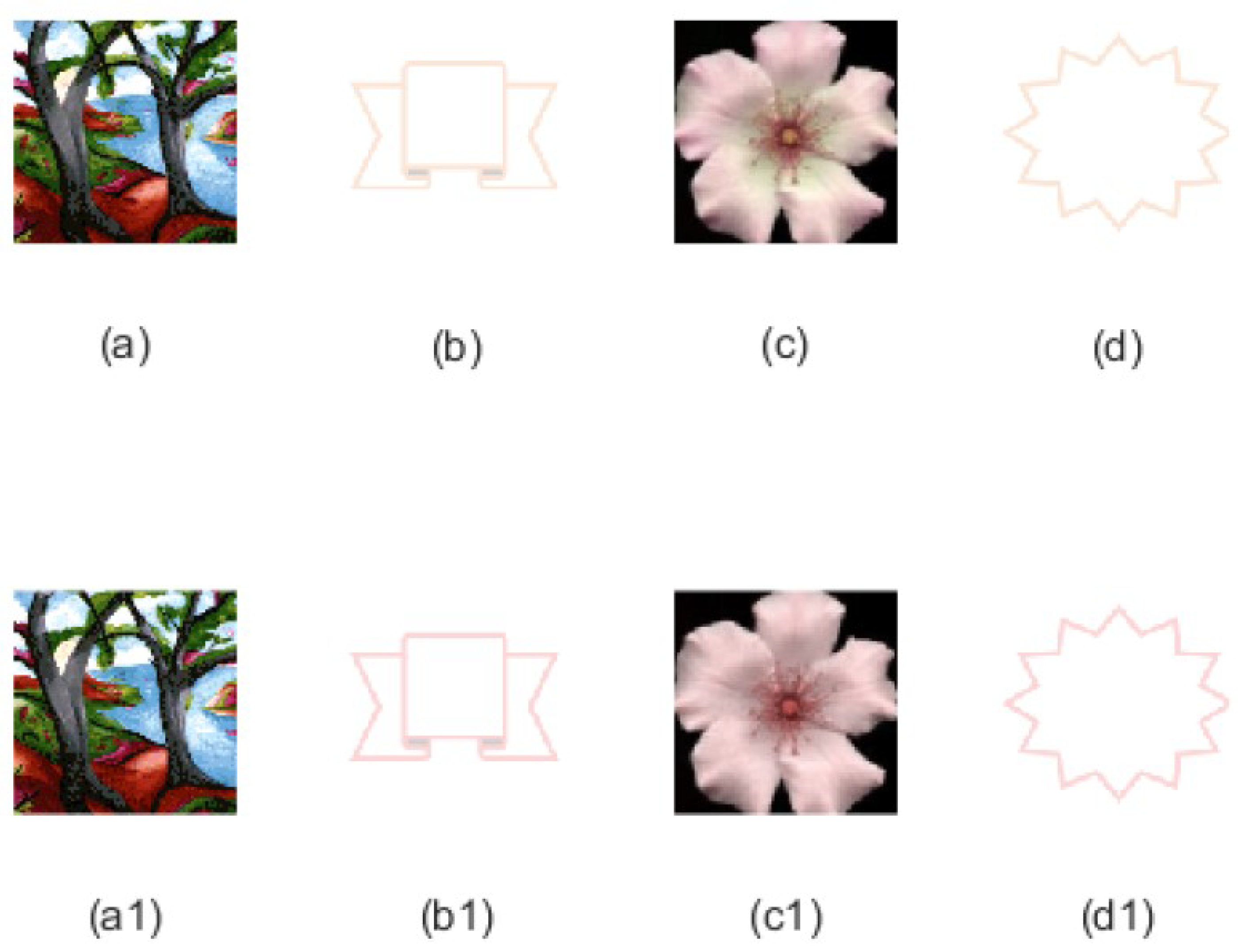
In this experimentation, we use the color images trees of

512 \times 512

pixels as the host images, and three color images as the watermarks to be implanted, which have the same size

128 \times 128

. Choosing scaling factor

α = 0.05

for T-RSVD-based method, we use the above frameworks to deal with the actual color image watermarking problem by the discrete wavelet transform (DWT) [16]. The experimental result of the T-RSVD-based color image watermarking shows in Figure 3.

PSNR values indicate that the T-RSVD-based color image watermarking have the dependable imperceptibility and security. Furthermore, as can be seen from Figure 3, the information before and after processing is very consistent. These results clearly show that the proposed methods fully satisfy the requirements for imperceptibility and security.

The color watermark processing framework based on T-RSVD has the following advantages. First, three color watermarks can be handled concomitantly. Secondly, only two keys need to be stored, and three color watermarks can be extracted. Furthermore, through the numerical experiment, it can be seen that the proposed methods have the responsible imperceptibility and security.

5. Conclusions

We have derived the restricted singular value decomposition (T-RSVD) for three tensors under t-product. We have demonstrated the algorithms, as well as an application from color watermark processing.

Author Contributions

All authors have equal contributions in conceptualization, formal analysis, investigation, methodology, software, validation, writing an original draft, writing a review, and editing. All authors have read and agreed to the published version of the manuscript.

Funding

This research is supported by the National Natural Science Foundation of China [grant number 12371023, 12271338]. The first author is also supported by the China Scholarship Council [grant number 202106890041].

Institutional Review Board Statement

Not applicable.

Informed Consent Statement

Not applicable.

Data Availability Statement

Not applicable.

Acknowledgments

The authors would like to thank the editor and reviewers for their valuable suggestions, comments, and the Natural Science Foundation of China under grant No. 12371023, 12271338. The first author would also like to appreciate the China Scholarship Council for funding his research at the National University of Singapore, Singapore.

Conflicts of Interest

The authors declare no conflict of interest.

References

Chu, D.; De Lathauwer, L.; De Moor, B. On the computation of the restricted singular value decomposition via the cosine-sine decomposition. SIAM Journal on Matrix Analysis and Applications 2000, 22(2), 580–601.
Comon, P.; Luciani, X.; De Almeida, A.L. Tensor decompositions, alternating least squares and other tales. Journal of Chemometrics: A Journal of the Chemometrics Society 2009, 23(7–8), 393–405.
De Lathauwer, L.; De Moor, B.; Vandewalle, J. A multilinear singular value decomposition. SIAM journal on Matrix Analysis and Applications 2000, 21(4), 1253–1278.
De Moor, B.L.; Golub, G.H. The restricted singular value decomposition: properties and applications. SIAM Journal on Matrix Analysis and Applications 1991, 12(3), 401–425.
Doostan, A.; Iaccarino, G.; Etemadi, N. A least-squares approximation of high-dimensional uncertain systems. Annual Research Briefs, Center for Turbulence Research, Stanford University 2007, 121–132.
Hao, N.; Kilmer, M.E.; Braman, K.; Hoover, R.C. Facial recognition using tensor-tensor decompositions. SIAM Journal on Imaging Sciences 2013, 6(1), 437–463.
Harjito, B.; Prasetyo, H. False-positive-free GSVD-based image watermarking for copyright protection. 2016 International Symposium on Electronics and Smart Devices (ISESD) 2016, 143–147.
He, Z.H.; Ng, M.K.; Zeng, C. Generalized singular value decompositions for tensors and their applications. Numerical Mathematics: Theory, Methods and Applications 2021, 14(3), 692–713.
Jin, H.; Bai, M.; Benítez, J.; Liu, X. The generalized inverses of tensors and an application to linear models. Computers and Mathematics with Applications 2017, 74(3), 385–397.
Kilmer, M.E.; Braman, K.; Hao, N.; Hoover, R.C. Third-order tensors as operators on matrices: A theoretical and computational framework with applications in imaging. SIAM Journal on Matrix Analysis and Applications 2013, 34(1), 148–172.
Kilmer, M.E.; Martin, C.D. Factorization strategies for third-order tensors. Linear Algebra and its Applications 2011, 435(3), 641–658.
Kolda, T.G.; Bader, B.W. Tensor decompositions and applications. SIAM review 2009, 51(3), 455–500.
Martin, C.D.; Shafer, R.; LaRue, B. An order-p tensor factorization with applications in imaging. SIAM Journal on Scientific Computing 2013, 35(1), A474–A490.
Miao, Y.; Qi, L.; Wei, Y. T-Jordan canonical form and T-Drazin inverse based on the T-product. Communications on Applied Mathematics and Computation 2021, 3, 201–220.
Miao, Y.; Qi, L.; Wei, Y. Generalized tensor function via the tensor singular value decomposition based on the T-product. Linear Algebra and its Applications 2020, 590, 258–303.
Lai, C.C.; Tsai, C.C. Digital image watermarking using discrete wavelet transform and singular value decomposition. IEEE Transactions on instrumentation and measurement 2010, 59(11), 3060–3063.
Omberg, L.; Golub, G.H.; Alter, O. A tensor higher-order singular value decomposition for integrative analysis of DNA microarray data from different studies. Proceedings of the National Academy of Sciences 2007, 104(47), 18371–18376.
Savas, B.; Eldén, L. Handwritten digit classification using higher order singular value decomposition. Pattern recognition 2007, 40(3), 993–1003.
Shashua, A.; Hazan, T. Non-negative tensor factorization with applications to statistics and computer vision. Proceedings of the 22nd international conference on Machine learning 2005, 792–799.
Song, G.; Ng, M.K.; Zhang, X. Robust tensor completion using transformed tensor singular value decomposition. Numerical Linear Algebra with Applications 2020, 27(3), e2299.
Zhang, J.; Saibaba, A.K.; Kilmer, M.E.; Aeron, S. A randomized tensor singular value decomposition based on the t-product. Numerical Linear Algebra with Applications 2018, 25(5), e2179.
Zeng, C.; Ng, M.K. Decompositions of third-order tensors: HOSVD, T-SVD, and Beyond. Numerical Linear Algebra with Applications 2020, 27(3), e2290.

Figure 1. Schematic diagram for watermark embedding.

Figure 2. Schematic diagram for watermark extraction.

Figure 3. Result of the T-RSVD-based color image watermarking with

α = 5

. (a) Host color image, (b) color watermark image 1, (c) color watermark image 2, (d) color watermark image 3, (a1) watermarked color image (PSNR=38.8733), (b1) extracted watermark 1 (PSNR=39.8408), (c1) extracted watermark image 2 (PSNR=32.7493), (c1) extracted watermark image 3 (PSNR=40.5018).

Figure 3. Result of the T-RSVD-based color image watermarking with

α = 5

Disclaimer/Publisher’s Note: The statements, opinions and data contained in all publications are solely those of the individual author(s) and contributor(s) and not of MDPI and/or the editor(s). MDPI and/or the editor(s) disclaim responsibility for any injury to people or property resulting from any ideas, methods, instructions or products referred to in the content.

© 2024 by the authors. Licensee MDPI, Basel, Switzerland. This article is an open access article distributed under the terms and conditions of the Creative Commons Attribution (CC BY) license (http://creativecommons.org/licenses/by/4.0/).

Copyright: This open access article is published under a Creative Commons CC BY 4.0 license, which permit the free download, distribution, and reuse, provided that the author and preprint are cited in any reuse.

MDPI Initiatives

Important Links

Choose an area of interest and we will send you notifications of new preprints at your preferred frequency.

Disclaimer

Restricted Singular Value Decomposition for a Tensor Triplet under T-product and Its Applications

Abstract

1. Introduction

2. Preliminaries

3. Restricted singular value decomposition for three tensors

4. An application from color image watermarking processing

5. Conclusions

Author Contributions

Funding

Institutional Review Board Statement

Informed Consent Statement

Data Availability Statement

Acknowledgments

Conflicts of Interest

References

MDPI Initiatives

Important Links

Subscribe