1. Introduction
The Gumbel distribution was and remains one of the most used statistical distributions in the frequency analysis of extreme events in hydrology. This aspect is mainly due to the simple parameter estimation expressions, as well as the simple and accessible expression of the quantile function (inverse function). In hydrology, the applicability of the Gumbel distribution is diverse, being mainly used for frequency analysis of maximum flows [
1,
2,
3,
4,
5,
6,
7,
8,
9,
10,
11,
12,
13,
14,
15,
16,
17,
18,
19,
20,
21,
22,
23,
24,
25,
26,
27,
28,
29,
30,
31,
32,
33,
34,
35,
36,
37,
38,
39,
40,
41,
42], maximum precipitation and the construction of IDF curves [
43,
44,
45,
46,
47,
48,
49,
50,
51,
52,
53,
54,
55,
56,
57,
58], minimum flows [
59,
60,
61,
62,
63,
64], etc.
The main and only advantage of the Gumbel distribution is the simplicity and accessibility of expressions and relationships. Regarding the disadvantages, we can state as the main disadvantage the limited flexibility of this distribution in modeling various skewness, which generally leads to the limitation of the application of this distribution. It is a distribution whose statistical indicators have constant values, namely: skewness
and kurtozis
for the method of ordinary moments (MOM) [
1,
2,
3,
4], L-skewnes
and L-kurtozis
for the method of linear moments (L-moments) [
1,
2,
3,
4,
65,
66,
67,
68], LH-skewness
and LH-kurtozis
for the method of high-order linear moments 1 (LH1-moments), respectively
and
for the method of high-order linear moments 2 (LH2-moments). Another major disadvantage is that for certain values of the coefficient of variation (
), is that the values generated in the field of high exceeding probabilities are negative. Thus for a coefficient of variation
the distribution generates negative values in the range of 87%-99.9%, for
negative values appear in the range 75%-99.9%, respectively for
negative values are found in the range 66%-99.9%.
Regarding the use of the Gumbel distribution with different parameter estimation methods, it was applied using the method of ordinary moments (MOM) [
1,
2,
3,
4,
5], the method of linear moments (L-moments) [
2,
64,
65,
66,
67,
68], the method of linear moments high order (LH-moments) [
69,
70,
71,
72,
73], weighted moments method (PWM) [
2,
74,
75], maximum likelihood method (MLE) [
2,
74,
75], least squares method (LSM) [
2,
74,
76,
77], weighted least squares method (WLSM) [
77], entropy method (ENT) [
76,
78], mixed moments method [
2,
74,
76].
Thus, the main objective of this manuscript is to analyze the limited applicability of this Gumbel distribution in determining the maximum flows on different particular cases of rivers, with different morphological, statistical and hydrological characteristics. The differences and the behavior of the curves of the inverse distribution function, estimated with the 9 previously mentioned methods, are highlighted. Regarding the Bayesian approach, this is not treated in this manuscript because, although important contributions have been made, it remains a method with limitations, being strongly influenced by subjective aspects in the choice of the a priori distribution, requiring complex analyzes and strong hypotheses for its choice [
79,
80,
81,
82].
Considering that ‘’in flood frequency analysis (FFA) may result in significant jumps in the estimates of design (flood) quantiles along with the lengthening series of maximum flows’’ [
83], the biases of the quantiles of the distribution (sampling analysis) due to the variability of the analyzed data lengths for two of the most used parameter estimation methods are presented: MOM and L-moments. These also represent the main methods of parameter estimation in the regionalization analyzes of extreme events because they are characterized by statistical indicators (arithmetic mean, mean square deviation, skewness and kurtosis) that can be determined regionally.
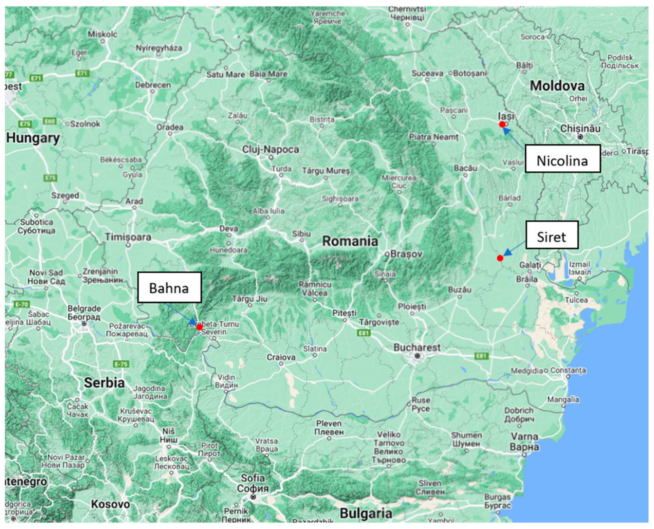
Regarding the FFA, 3 rivers related to the territory of Romania are analyzed using the series of maximum annual flows (AMS), with morphometric characteristics (watershed areas, average slopes, average altitudes, sinuosity, etc.), statistical and hydrological characteristics (long-gimi data available, coefficient of variation, skewness and kurtosis) different.
The results of the case studies are presented compared to those obtained with two other much more flexible distributions, such as the GEV distribution and the four-parameter Wakeby/Burr distribution, with parameters estimated using the L-moments method. The choice of the L-moments method as a reference is due to the main advantages, presented and highlighted in many scientific materials [
65,
68,
69,
70,
84,
85,
86,
87,
88,
89,
90], namely: robust in estimating statistical indicators and in estimating parameters and quantiles of distributions at the variability of data lengths, as well as the presence of outlier values. Also, the method presents rigorous criteria for choosing the best model, namely compliance with the conditions that the higher-order statistical indicators (L-skewness and L-kurtosis) specific to the chosen distribution come as close as possible to the corresponding ones of the analyzed data [
2,
68,
71,
72,
87,
88,
89,
90,
91,
92]. The comparison with the values generated by the Burr distribution was based on the consideration that this, being characterized by 4 parameters, manages the exact calibration of all four linear moments, the results obtained being characterized by a high degree of confidence. In previous materials [
91] it was demonstrated that by choosing the appropriate distribution of two parameters, by observing the specific criteria of the L-moments method, the errors in the estimation of quantiles can be greatly reduced. If it is desired to use a two-parameter distribution, it is recommended to use the L-moments method, and the preselection of the distributions and the selection of the model distribution should be done according to the criteria specific to the method, namely according to the values and variation curves (diagrams of variation) of the L-skewness and L-kurtosis indicators. In the last period, numerous relations and diagrams of variations were developed and presented for a significant number of two- and three-parameter distributions [
71,
72,
73,
87,
88,
89,
90,
91,
92,
93,
94].
Regarding the determination of the maximum annual precipitation, the performances of the Gumbel distribution are analyzed on two case studies with different statistical, mathematical and hydrological peculiarities.
Considering that in the frequency analysis we want to forecast the values corresponding to rare and very rare events (annual exceedance probability, p<1%), characteristic of long return periods (average return period, T>100 years), the performance of the Gumbel distribution is analyzed on two distinct levels of the maximum annual probabilities of non-exceedance, namely on the interval between p1%~p100%, in the case of maximum precipitation (hp), where data are generally available and generally the value of the quantile with an average return period of 200 years is of interest, respectively for the interval p0.01%~p1%, in the case of maximum flows (Qp), where most of the time there is no data available, representing the interval in which the extrapolation analysis of the available data is desired. These values from the FFA are of particular importance as they represent the flows necessary for the design of dam-type hydrotechnical constructions. Determining them accurately leads to the avoidance of additional costs which in some cases are significant (leading to the over-dimensioning of protection works), respectively the avoidance of loss of human life and important damages due to the under-dimensioning of the design flows that can generate a failure.
Among the most important new contributions made in the manuscript, regarding the Gumbel distribution and the methods of using it in the analysis of extreme events, I mention: 1) Presentation of the relationships for estimating the parameters and frequency factors of the Gumbel distribution using the 1st and 2nd order LH-moments method; 2) Presentation of the systematic biases of the Gumbel distribution (for both parameters and quantiles) depending on the statistical variability of extreme events (statistical indicators, available string lengths) for the most common parameter estimation methods; 3) A comparative analysis regarding the behavior of the Gumbel distribution for a significant number of parameter estimation methods; 4) Establishing clear and rigorous recommendations regarding the applicability and usefulness of the Gumbel distribution.
It is for the first time that a comparative analysis is performed regarding the applicability of the Gumbel distribution, using so many parameter estimation methods. This information and the obtained results will help researchers to use this statistical distribution appropriately and rigorously.
2. Methods
This section presents in detail the statistical and mathematical elements necessary to apply the Gumbel distribution using the 9 methods of estimating the analyzed parameters. The variation graphs of the inverse function related to the variability of the available data lengths and the data variability (the theoretical choice of the usual Cv in FFA) are also presented, highlighting the systematic biases of the distribution for the annual maximum values (with MOM and L-moments) for the annual exceedance probabilities of interest: 1%, 0.1% and 0.01% [
1,
2,
71,
72,
73].
This analysis, of the evidence of the systematic biases of the distribution, follows the stage of choosing the best model. In this second stage, it is considered that the analyzed values (observed data) are drawn from a Gumbel distribution.
2.1. Estimating the parameters of the Gumbel distribution.
The Gumbel distribution is a particular case of the Generalized Extreme Value (GEV) distribution when the shape parameter
[
1,
2,
3,
4]. It is also known as the type I extreme value distribution, the LogWeibull distribution, the Fisher-Tippett type I distribution or the Gompertz distribution [
95].
The probability density function, the complementary cumulative function and the quantile function of the Gumbel distribution have the following expressions [
1,
2,
3,
4,
64,
66,
67,
74]:
where,
is the scale parameter, and
is the position parameter;
.
Functia cuantila mai poate fi exprimata, pentru MOM, L- and LH-moments, utilizand factorul de frecventa () astfel:
where
is the arithmetic mean (expected value),
represents the variation, and
is Euler's constant;
and
represent the first two linear moments;
and
represent the first two high order linear moments.
2.1.1. Method of Ordinary Moments (MOM).
The conditions and expressions of the parameters of the Gumbel distribution using MOM are as follows [
1,
2,
67]:
The two expressions of the distribution parameters result from equations (7) and (8):
The frequency factor of the distribution using the MOM method is defined [
2,
87]:
2.1.2. The method of linear moments (L-moments)
To determine the expressions of the parameters using the L-moments method, it is necessary to impose the following two conditions [
2,
67,
74,
87]:
The expressions of the two parameters are the following:
The frequency factor of the distribution using the L-moments method has the following explicit form:
2.1.3. The method of high-order linear moments (LH-moments)
The equations of the conditions necessary to estimate the parameters using the method of linear moments of order 1 (LH1-moments) are the following:
The position and scale parameters have the following expressions:
The frequency factor of the distribution using the LH1-moments, is:
In the case of the method of linear moments of order 2, the two conditions are:
It follows from equations (22) and (23) that:
The frequency factor of the distribution using the LH2-moments, is:
2.1.4. The probability weighted moment method (PWM)
The general equation for obtaining the weighted moments has the following mathematical expression [
2,
74,
75]:
where
represents the length of the analyzed data string;
is the string of recorded values in ascending order;
is the chosen empirical probability;
. For
we get the expected value.
Like the least squares method (LSM), this also has an important subjective component by choosing the empirical probability.
The parameter equations are:
2.1.5. The method of maximum likelihood estimation(MLE)
The relations for estimating parameters with MLE are the following [
2,
74,
76,
77]:
2.1.6. The least squares method (LSM)
To determine the parameters using the LSM method, it is necessary to solve the following system of nonlinear equations [
76]:
2.1.7. The weighted least squares method (WLSM)
The nonlinear equations of the system needed to estimate the parameters with WLSM are the following [
76]:
2.1.8. The entropy weight method (ENT)
The scale parameter is obtained by finding the solution of the following nonlinear equation [
76]:
With the scale parameter thus known, the position parameter is determined using the equation (31).
2.1.9. The method of mixed moments (MIX)
The equations for determining the parameters using the MIX method have the following expressions [
76]:
Regarding the estimation of the parameters of the four-parameter Burr and five-parameter Wakeby distributions using the L-moments method, they are presented in previous materials [
91,
93].
2.2. Systematic biases due to the variability of data lengths
This section presents, for the Gumbel distribution, a comparative analysis of the behavior of the quantile function (in the field of low exceedance probabilities, events with a long return period), depending on the number of values () and depending on the coefficient of variation (), for different empirical probabilities () chosen in the sampling. The biases of the distribution parameters are highlighted, as well as the biases of the values generated for four small annual non-exceedance probabilities (p=0.01%, 0.1%, 1% and 5%), compared to the theoretical values (n>1000 values) characteristic of the Gumbel distribution.
The analysis is done by sampling, using the inverse function (with parameters estimated on the theoretical values, n>1000) and Hazen empirical probability. The choice of the best empirical probability for sampling was made so that the differences between the generated values and the theoretical ones are minimal. This must be established, depending on the parameter estimation method and the analyzed distribution [
96]. The influence of the choice of the empirical probability is thus presented, aspects that also influence the estimation of the parameters using the LSM or PWM methods. A number of 13 empirical probabilities were analyzed [
2,
96], namely Blom, Weibull, Beard, Hazen, Cunnane, Gringorten, Adamowski, Chegodayev, Filliben, Hirsch, IEC56, McClung & Mears, Landwehr/APL.
2.2.1. Method of ordinary moments
Being a two-parameter distribution, the MOM analysis is based on the theoretical values of the coefficient of variation (
). In general, in frequency analysis in hydrology, it takes values between 0.1 and 5. Regarding the sampling (both for MOM and for L-moments) this is done for a number of values of
, lengths generally available in real data applications. In
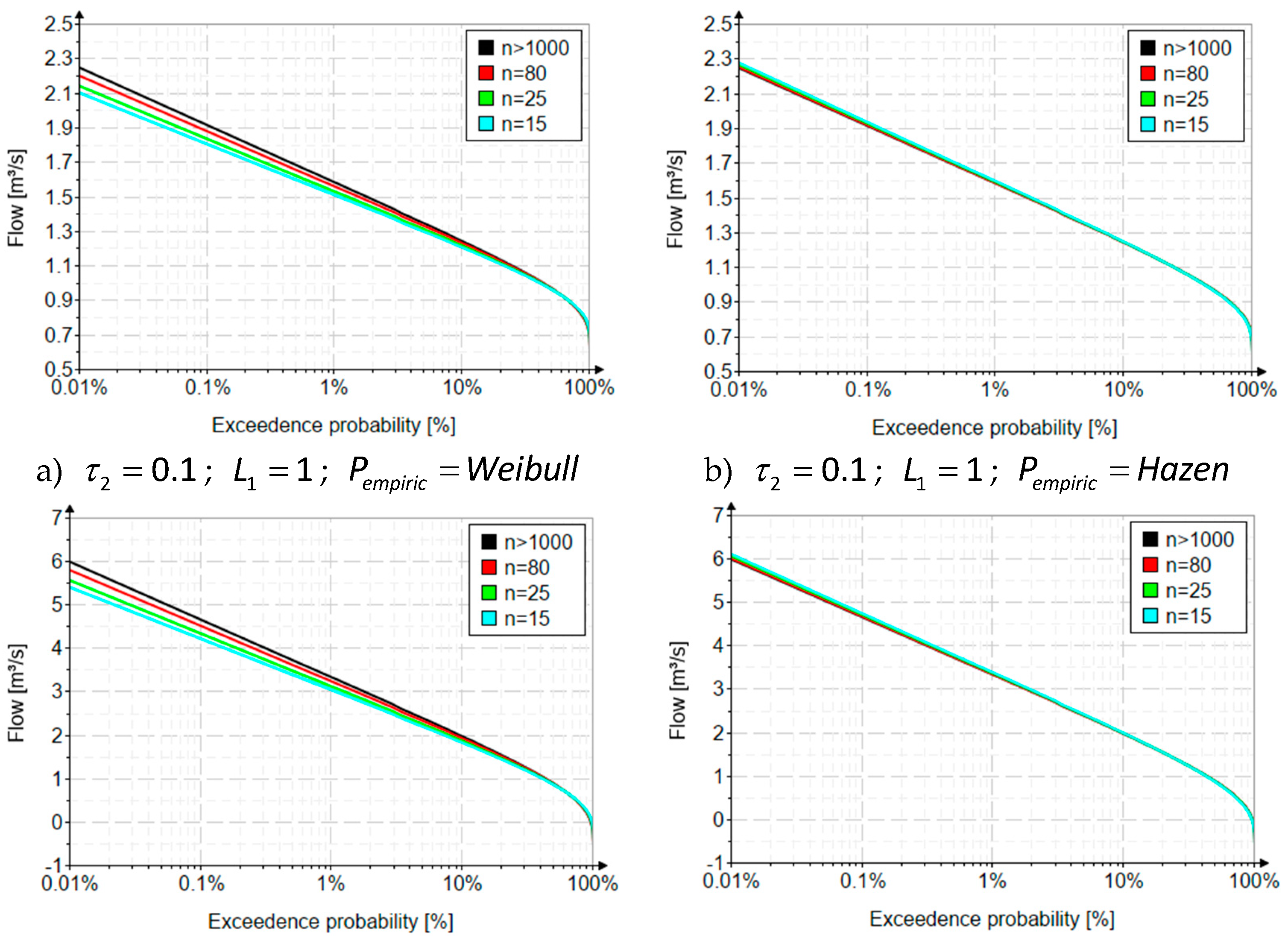
Figure 1 are presented the graphs of the behavior of the inverse function, for different values of the coefficient of variation and according to the empirical probabilities that generated the largest biases (Weibull), respectively the smallest (Hazen).
The theoretical bias values in estimating the parameters of the Gumbel distribution, for all the analyzed values (data lengths and coefficient of variation values) are presented, as a percentage, in
Table 1 and
Table 2.
An interesting aspect was highlighted by Gaume [
79], namely the transmission of the parameter biases in the quantile biases, this being influenced by the parameter estimation functions specific to the MOM and L-moments method.
Thus, the
Table 3 show these systematic biases in estimating the parameters of the Gumbel distribution.
2.2.2. The method of linear moments
In the case of L-moments, the systematic biases are influenced by the coefficient of L-variation
, which is the counterpart of the MOM specific coefficient of variation, but estimated using the first two linear moments. The coefficient of L-variation always takes values between 0 and 1 [Hosking, two parameters]. In this situation, 4 values (0.1, 0.4, 0.6 and 0.8) were chosen to include a diversified variability, from small to large.
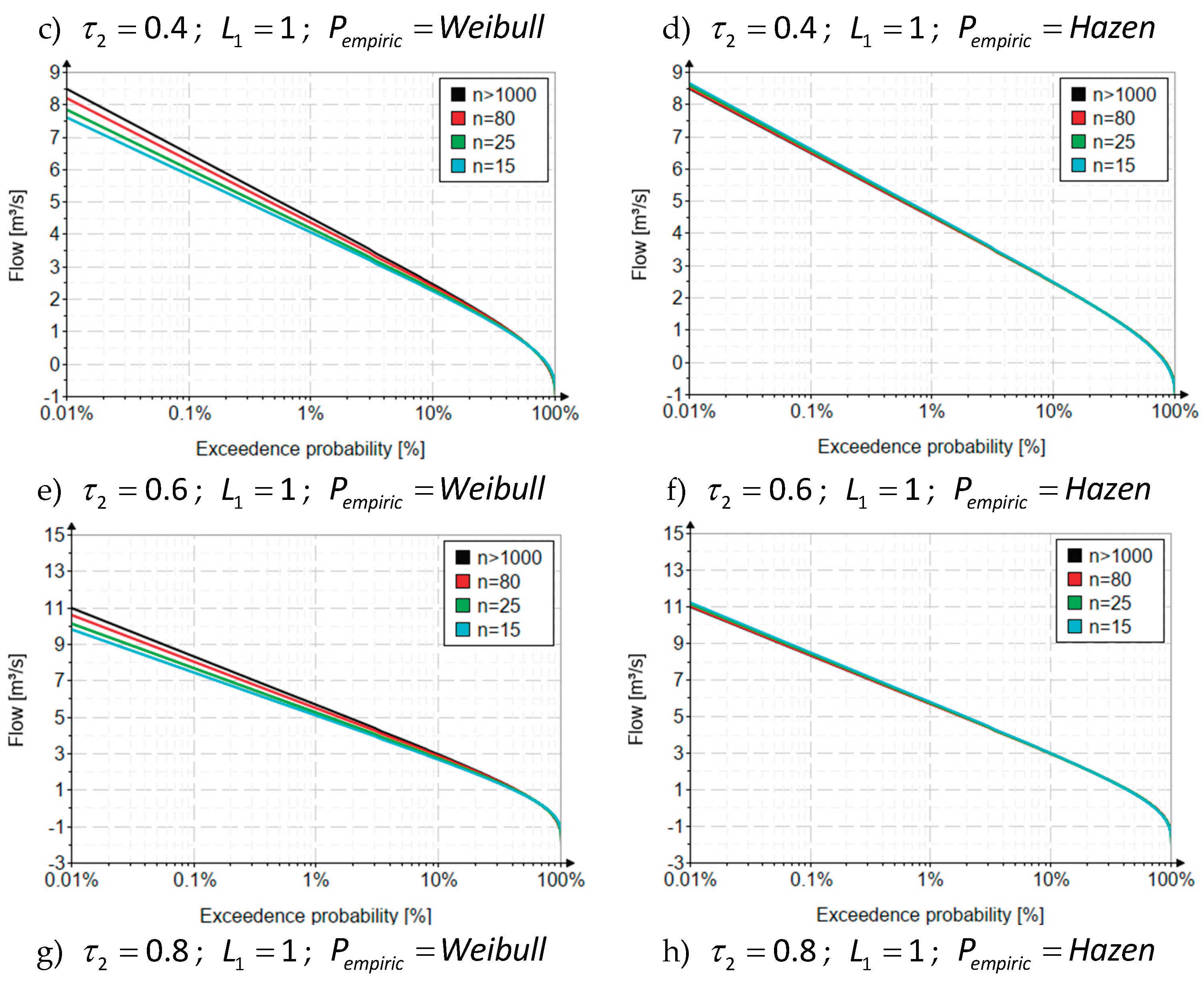
Figure 2 shows the results of the inverse functions obtained for the analyzed cases.
As in the case of the method of ordinary moments, the theoretical biases will be highlighted both in the estimation of the parameters and in the estimation of the quantile values related to the event with the average return period T=10000.
Table 4 and
Table 5 show the biases related to the two parameters of the distribution.
Table 6 present the systematic biases obtained with L-moments for the value of the quantile related to the annual exceedance probabilities of interest.
2.3. Choosing the best model
In general, choosing the best model involves two components, namely one subjective and one objective. For the vast majority of parameter estimation methods (MOM, MLE, PWM, LSM, WLSM, ENT, MIX, ) the subjective component is the predominant one because there are no rigorous criteria for choosing the best model, it being chosen based on the results of the application of indicators and performance tests, the results of which are applicable and can only be interpreted in the area of the annual probabilities of exceeding the observed values. Outside of this field (in general, data is wanted to be forecast there) they can no longer constitute a selection criterion, because they are based only on the difference between generated and observed (recorded, real) values.
In the case of the L-moments method, there are clear criteria for selecting the best model, namely the calibration of the indicator values of L-skewness (
) and L-kurtozis (
) of the observed data [
2,
65,
66,
67,
69,
71,
72,
73,
87,
88,
89,
90,
91,
92,
93,
94]. Unfortunately, the Gumbel distribution is not defined, like the two-parameter Log-normal or Gamma distribution, by a variation curve of these indicators, but has constant values regardless of the observed data analyzed [
91]. On the general graphs of variation of the indicators obtained with the L-moments method, this is defined by a point [
2,
65,
91].
Thus, in the case of FFA, the selection of the best model is based on the selection criteria of the L-moments method, while in the case studies regarding the maximum determination of precipitation, the selection is based on both the L-moments criteria and performance indicators, because the values of the quantiles related to the interested probabilities are approximated by the empirical ones of the recorded data, in general there are recorded data in this field.
4. Results and Discussions
The results and the discussions regarding the obtained results are mainly focused on two important directions, namely: 1) verification of the applicability of the Gumbel distribution in the field of maximum flow frequency analysis (FFA), where the analysis focuses on the quantile values in the field of low exceedance probabilities (p <1%), because in FFA these are the values that want to be forecasted. Both in Romanian and international legislation (ICOLD) in the design of hydrotechnical constructions, it is necessary to directly determine the values of the quantiles of the following annual exceeding probabilities: 0.01%, 0.1%, 0.5%, 1%, 2%, 5%, 10%, depending on the importance class of the construction [STAS 4068/2-87; Annual probabilities of maximum flows and volumes under normal and special operating conditions. The Romanian Standardization Institute: Bucharest, Romania, 1987.]; and 2) verifying the applicability of the Gumbel distribution in the direct determination of the maximum precipitation values for return periods of up to 500 years (p=0.2%), values generally required for the construction of IDF curves.
4.1. Flood Frequency Analysis
In all the case studies, the values generated by the Gumbel distribution are analyzed compared to the Burr reference distribution and the L-moments reference method, for the reasons stated in the previous Sections: the Burr distribution has a large number of parameters, managing to properly calibrate all the linear moments; the L-moments method is superior to the other estimation methods. Additionally, for the rigor of the analysis, another distribution with a high number of parameters is used, namely the Wakeby distribution.
4.1.1. Verification of normality
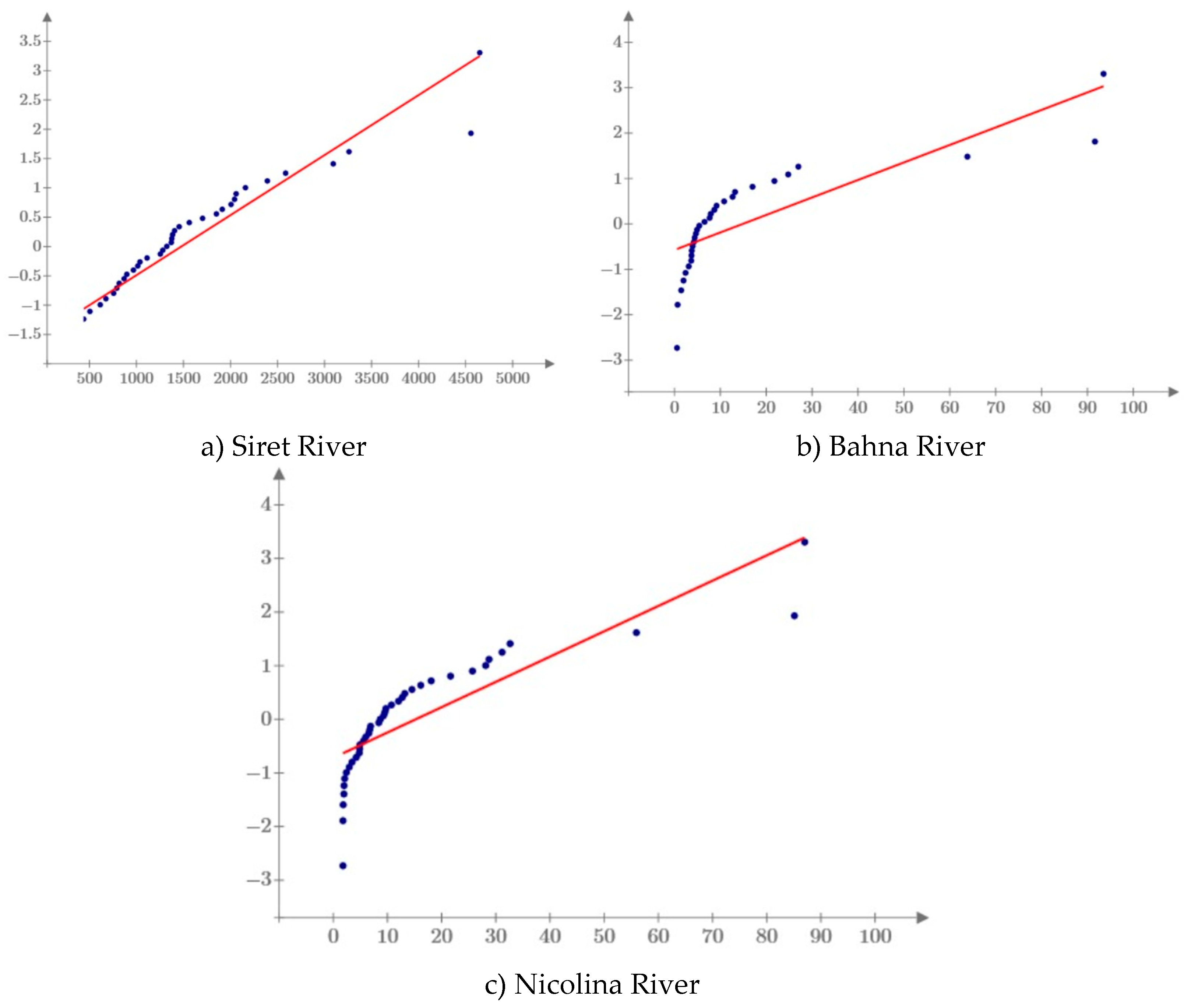
The verification of the normality of the data was done graphically (see
Figure 9), being able to easily notice that the observed data do not come from a normal distribution.
In all three cases it can be observed that the recorded values have a heavy-tailed tendency.
4.1.2. The verification of stationarity and outliers
Stationarity was checked using the "t" test. Its results as well as the critical values are presented in Table11. No non-stationarity of the analyzed data is observed. Outliers were checked using the Grubbs test, no outliers were identified in the analyzed data series.
4.1.3. Statistical analysis on the field of recorded data
The graphic verification of the correlation (Q-Q plot) of the observed data with those generated by the analyzed distributions, with the estimated parameters using the L-moments method, are presented in
Figure 10,
Figure 11 and
Figure 12.
It can be observed that, in all three case studies, the Burr, GEV and Wakeby distributions have the best results, the values generated by them being the closest to those of the recorded data. The additional use of some tests (Kolmogorov-Smirnov, Anderson Darling, etc.) and performance indicators (RAE, RME, RMSE, etc.) would highlight the same situation observed graphically.
4.1.4. Statistical analysis on the field of low annual exceedance probabilities.
Considering the values of the quantiles related to the annual exceedance probabilities that are to be determined, this analysis is the most important. It also represents the field in which there is a diverse and different behavior of statistical distributions, imposed by the type of distribution (number of parameters and the family it belongs to), the parameter estimation method and the available lengths of the observed data.
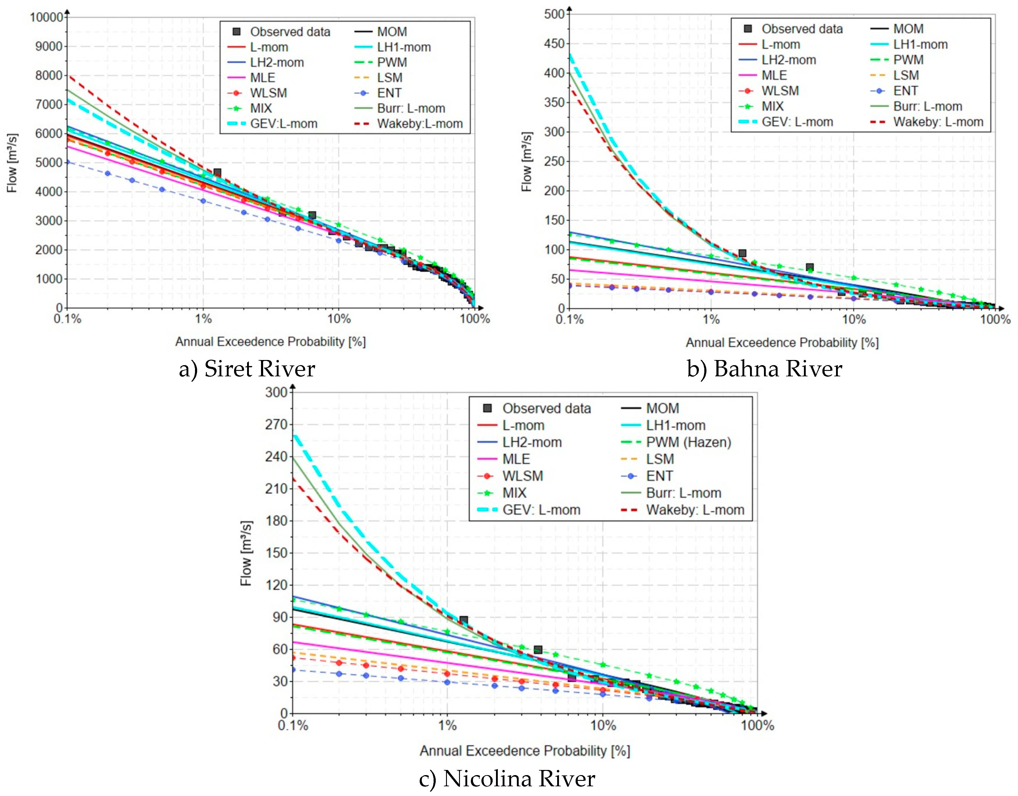
In the case of the three case studies, the variation graphs of the inverse function (quantile function), related to each distribution and estimation methods of the analyzed parameters, are presented in
Figure 13.
It can be seen that the values generated by the Gumbel distribution, regardless of the parameter estimation method used, are much lower than the GEV, Burr and Wakeby distributions, which have a larger number of parameters, thus managing to calibrate the higher-order linear moments.
Analyzing the values generated for the annual probability of exceeding 0.1%, it can be seen that the quantile values of the Gumbel distribution vary in the range of 5000-6500 mc/s for the Siret River, between 38-130 mc/s for the Bahna River, respectively between 40-120 mc/s and in the case of the Nicolina River. In all analyzed cases, the lower values were generated by the entropy method (ENT), while the higher values were generated by estimating the parameters with the 2nd order linear moments method. For the same annual probability of non-exceedance (0.1%), the values generated by the distribution GEV, having parameters estimated with the L-moments method, the values are 7157 mc/s for the Siret River, 429 mc/s for the Bahna River, respectively a value of 263 mc/s for the Nicolina River. The Burr (four-parameter) and Wakeby (five-parameter) distributions generated relatively close values, an aspect due to the possibility of these distributions to calibrate all the linear moments specific to the L-moments method. In the case of the Siret River, the generated values are between 7498 mc/s (Burr) and 8026 mc/s (Wakeby). In the case of the Bahna River, the values are between 379 mc/s (Wakeby) and 400 mc/s (Burr). For the data series related to the Nicolina River, the Burr distribution generated a value of 239 mc/s, and the Wakeby distribution a value of 220 mc/s.
It can be observed that the use of the Gumbel distribution, without respecting the calibration criteria imposed by the L-moments method, generates values characterized by very large errors for the values of the quantiles related to some rare events that want to be forecasted, especially if we take into account that in generally, in FFA, the direct determination of some events with a return period of up to 10,000 years is required, which leads to even greater forecast errors. Thus,
Table 12 shows the estimation errors of the quantile of the Gumbel distribution, having as reference the values generated by the Burr distribution (considered in these cases the "parent" distribution). For these case studies, the theoretical biases (relative errors from the behavior of the Gumbel distribution depending on the length of the available data series) are not highlighted because they are insignificantly smaller if we compare them to the errors from the selection of the best model. Very large errors can be observed which, in the case of inadequate analyzes and in the absence of a rigor of these analyses, can lead to the defective dimensioning of some hydrotechnical works which can lead to undesirable consequences, both economic but most importantly can indirectly lead to losses of human lives. This reasoning is also valid in the case of three-parameter distributions (Pearson III, GEV, Pareto, etc.) when they are not used and applied properly.
4.2. Annual Maximum Daily Rainfall (24h)
In the case of the analysis of the maximum annual precipitation, the values of the interested quantiles (hp) are those related to a maximum annual exceedance probability of 0.2% (T=500 years), 0.5% (T=200 years), 1% (T=100 years) and 2% (T= 50 years).
In general, for this interval of probabilities, the data series are long enough so that the errors in estimating the values with the Gumbel distribution are small. But there are also cases when the lines are not long enough, requiring a more laborious analysis in choosing the best model.
Thus, in this section, the criteria for choosing the best distribution consist in compliance with the conditions imposed by the L-moments method (also chosen in these cases as reference), but also in the use of some performance indicators that are based on highlighting the relative errors between recorded and forecasted values. For the two analyzed case studies, the RME (Relative Mean Error) and RAE (Relative Absolute Error) performance indicators are used.
4.2.1. Verification of normality
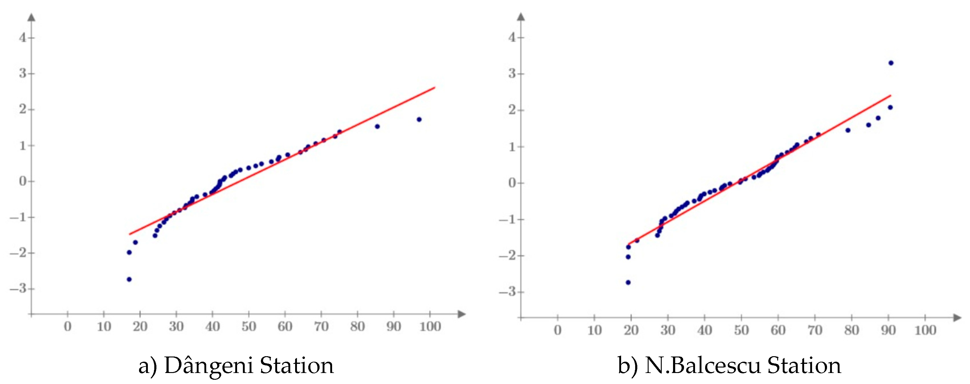
The normality of the data is verified graphically and presented in
Figure 14. It can be observed, that the data do not come from a normal distribution.
In both cases the observed values have a heavy-tailed tendency.
4.2.2. The verification of stationarity and outliers
Regarding the stationarity check, the results of the "t" test are presented in
Table 13, the values being lower than the critical ones, thus highlighting the stationarity of the analyzed data. An analysis was also carried out regarding the existence of outlier values (Grubb’s test), no such values being identified.
4.2.3. Analysis of forecasted values
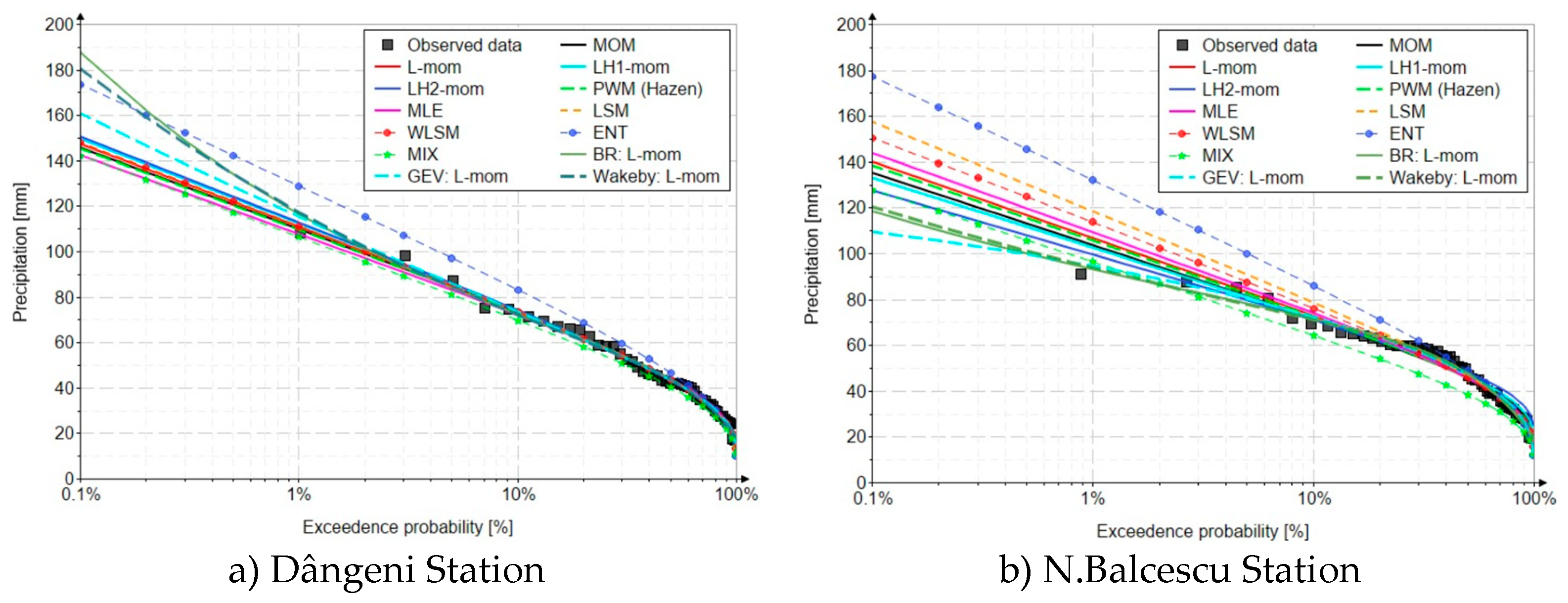
Figure 15 presents the results and behavior of the inverse functions of the analyzed distributions.
Analyzing the obtained results, it can be easily observed that the values generated by the four distributions differ significantly, for both case studies. The particular aspects of the obtained results are detailed in the next section.
4.2.3.1. Dângeni station results
In the case of the Dângeni Station, the values generated with the Gumbel distribution (reference probability, p=0.2%) are around the value of 136 mm, expect the value related to the estimate with the ENT method where the predicted value is 160 mm, but it can be easily observed that it practically does not pass through the points of the recorded values.
The values generated by the distributions with a high number of parameters vary between 147 mm (GEV distribution) and 162 mm (Burr and Wakeby distributions).
The results of the performance indicators are presented in the
Table 14. Analyzing the values, the GEV distribution has the best result. But considering that this is a relevant indicator only in the area of the probabilities of the recorded values, and the empirical probability related to the highest value (n=49) is 1.02%, the selection of the best model must be made respecting the criteria imposed by the reference method L - moments. Thus, following the analysis of the L-skewness and L-kurtosis statistical indicators, the Burr and Wakeby distributions are the ones that properly calibrate the similar values of the observed data, namely 0.2 and 0.153 respectively.
The relative errors between the values generated by the Gumbel distribution and those of the best model are presented in
Table 15. Its vary between -18.9% and -1.3% depending on the predicted probability.
4.2.3.2. N.Balcescu station
Like the Dângeni Station, the values of interest are those of the rarest event, namely the one with an annual probability of exceeding 0.2%. The Gumbel distribution generated values between 128 mm (LH-moments and MIX method) and 164 mm (ENT method). Even in this case, it can be observed that the values generated with the ENT method do not properly approximate the recorded values. For all parameter estimation methods, the values generated by the Gumbel distribution are superior to those generated by the GEV, Burr and Wakeby distributions. In the case of the GEV distribution, the corresponding p=0.2% value is 105 mm, while in the values generated by the Burr and Wakeby distributions, it is around 120 mm. Graphically, it can be seen that the curves of the three distributions pass through the points related to the observed data.
The performances of the distributions are presented in the
Table 16. Based on the results, the best model is the Burr distribution. This choice is also in accordance with the corresponding calibration of the higher order statistical indicators (L-skewness and L-kurtosis) specific to the L-moments method, namely 0.069 and 0.074, respectively. Very close values of RAE and RME are also generated by the Wakeby distribution, an aspect otherwise expected as both distributions fulfill specific calibration criteria of the L-moments method, an aspect partially due to the fact that the empirical probability related to the maximum value of the observed data (n=56) is 0.893 %, a value closer to the desired 0.2%, the data extrapolation interval being smaller.
Table 17 shows the errors between the values generated by the Gumbel distribution and those generated by the best model, namely the Burr distribution. It can be seen that the errors in the estimation of the best model are between 10.5% and 15.3%, increasing with the decrease of the annual probability of exceeding.
5. Conclusions
The Gumbel distribution was, is and will probably remain one of the most used statistical distributions in the analysis of extreme events in hydrology.
In the literature, this is used using different parameter estimation methods, among which the most common are the method of ordinary moments and the method of linear moments. Its applicability on a large scale is generally due to the simplicity of the equations needed to estimate the parameters, as well as the simplicity of the expression of the inverse function, being generally applied using the characteristic frequency factor.
Following the case studies presented in this manuscript, which contains 3 frequency analyzes in determining the maximum flows and two frequency analyzes of the maximum annual precipitation, with the parameters estimated with 9 methods, as well as following the observations based on the available scientific materials, it can be concludes that the real utility of the distribution is limited, its application can only be made if the conditions imposed by the parameter estimation methods are met.
Taking into account that among all the parameter estimation methods, the L-moments method proved to be the most robust and reliable method, being also the only method in the regionalization analyzes of extreme events in hydrology, it is recommended to use the Gumbel distribution with this method and only after a preliminary analysis regarding the most accurate calibration of the statistical indicators, L-skewness and L-kurtosis, as characteristics of the distribution with those of the analyzed data series. Compared to other two-parameter distributions (Gamma, Weibull, Log-normal, etc.), the Gumbel distribution has the great disadvantage that the values of these indicators do not fit on a variation curve of interdependence, but have constant values, namely: L-skewness and L-kurtosis .
Figure 1.
The variation curves of the inverse function at different series lengths and values of the coefficient of variation – method of ordinary moments.
Figure 1.
The variation curves of the inverse function at different series lengths and values of the coefficient of variation – method of ordinary moments.
Figure 2.
The variation curves of the inverse function at different series lengths and values of the coefficient of variation – method of linear moments.
Figure 2.
The variation curves of the inverse function at different series lengths and values of the coefficient of variation – method of linear moments.
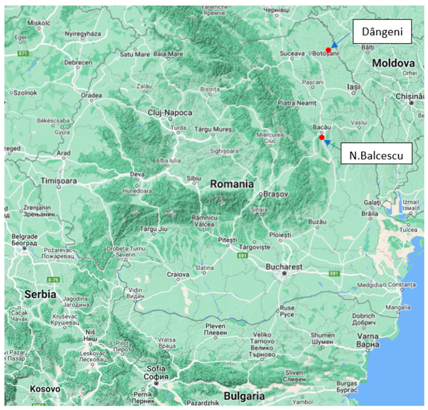
Figure 3.
The location of the studied rivers and hydrometric stations.
Figure 3.
The location of the studied rivers and hydrometric stations.
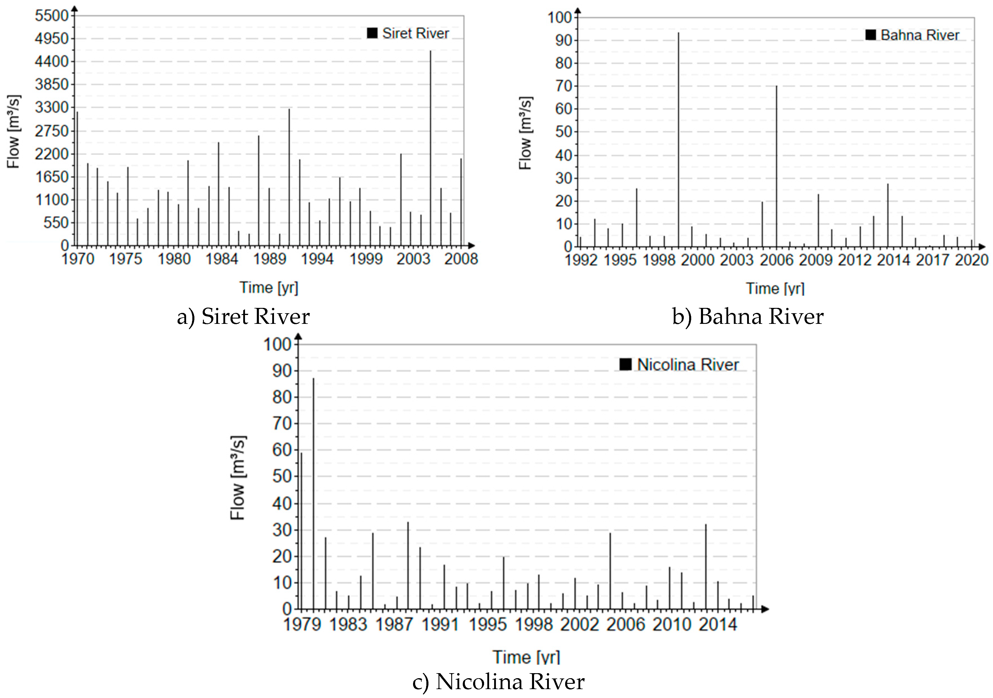
Figure 4.
The chronological series for the analyzed rivers.
Figure 4.
The chronological series for the analyzed rivers.
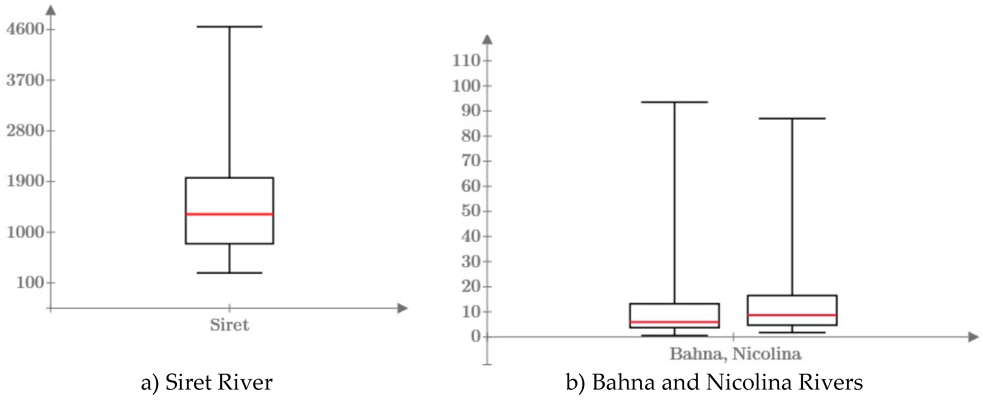
Figure 5.
The Box-plot representation of the analyzed series.
Figure 5.
The Box-plot representation of the analyzed series.
Figure 6.
The location of the studied Station.
Figure 6.
The location of the studied Station.
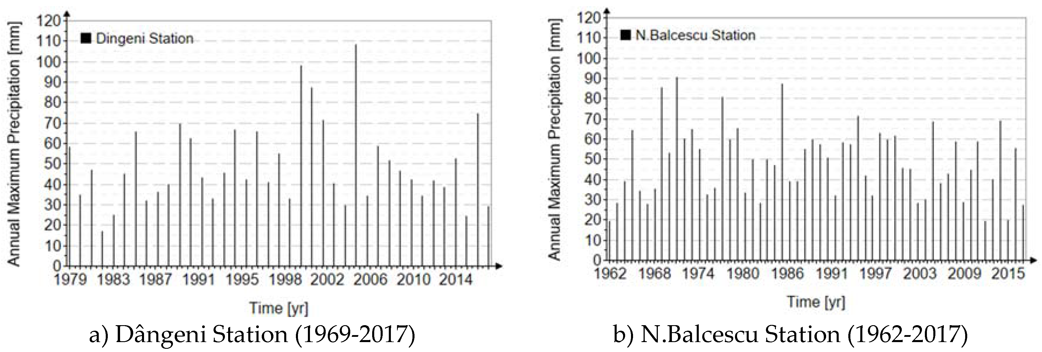
Figure 7.
The chronological series for the analyzed Stations.
Figure 7.
The chronological series for the analyzed Stations.
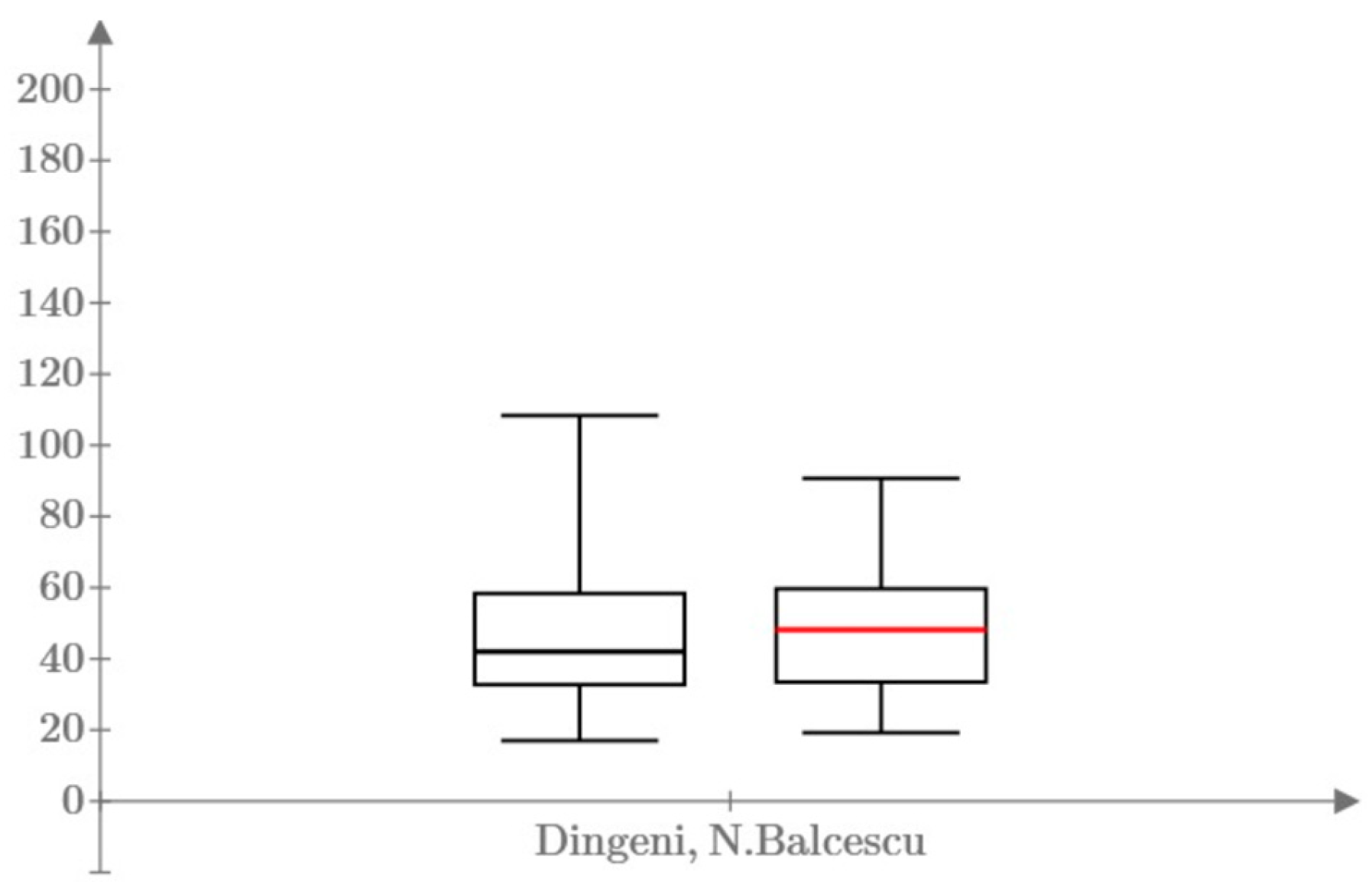
Figure 8.
The Box-plot representation for Dângeni and N. Balcescu series.
Figure 8.
The Box-plot representation for Dângeni and N. Balcescu series.
Figure 9.
Normal Q-Q Plot: Siret, Bahna and Nicolina Rivers.
Figure 9.
Normal Q-Q Plot: Siret, Bahna and Nicolina Rivers.
Figure 10.
Graphic correlation of data: Siret River.
Figure 10.
Graphic correlation of data: Siret River.
Figure 11.
Graphic correlation of data: Nicolina River.
Figure 11.
Graphic correlation of data: Nicolina River.
Figure 12.
Graphic correlation of data: Bahna River.
Figure 12.
Graphic correlation of data: Bahna River.
Figure 13.
Graphic representation of quantile functions for the Siret, Bahna and Nicolina Rivers.
Figure 13.
Graphic representation of quantile functions for the Siret, Bahna and Nicolina Rivers.
Figure 14.
Graphical verification of data normality: Dângeni and N.Balcescu Stations.
Figure 14.
Graphical verification of data normality: Dângeni and N.Balcescu Stations.
Figure 15.
The quantile functions results for the Dângeni and N.Balcescu Stations.
Figure 15.
The quantile functions results for the Dângeni and N.Balcescu Stations.
Table 1.
The theoretical biases for the scale parameter: MOM.
Table 1.
The theoretical biases for the scale parameter: MOM.
| The scale parameter β
|
| The coefficient of variation |
Number of values |
|
|
|
| Empirical probability |
| Weibull |
Hazen |
Weibull |
Hazen |
Weibull |
Hazen |
| Theoretical bias [%] |
|
6.33 |
1.07 |
13.15 |
2.57 |
17.63 |
3.69 |
|
6.33 |
1.07 |
13.15 |
2.57 |
17.63 |
3.69 |
|
6.33 |
1.07 |
13.15 |
2.57 |
17.63 |
3.69 |
|
6.33 |
1.07 |
13.15 |
2.57 |
17.63 |
3.69 |
|
6.33 |
1.07 |
13.15 |
2.57 |
17.63 |
3.69 |
Table 2.
The theoretical biases for the position parameter: MOM.
Table 2.
The theoretical biases for the position parameter: MOM.
| The position parameter γ
|
| The coefficient of variation |
Number of values |
|
|
|
| Empirical probability |
| Weibull |
Hazen |
Weibull |
Hazen |
Weibull |
Hazen |
| Theoretical bias [%] |
|
-0.13 |
-0.02 |
-0.24 |
-0.03 |
-0.31 |
-0.02 |
|
-1.04 |
-0.16 |
-1.89 |
-0.23 |
-2.4 |
-0.19 |
|
-2.3 |
-0.36 |
-4.19 |
-0.5 |
-5.3 |
-0.41 |
|
-25.31 |
-3.93 |
-46.09 |
-5.51 |
-58.39 |
-4.53 |
|
6.32 |
0.98 |
11.51 |
1.37 |
14.58 |
1.13 |
Table 3.
The theoretical biases for rare events (p = 0.01 %, 0.1 %, 1 % and 5%): MOM.
Table 3.
The theoretical biases for rare events (p = 0.01 %, 0.1 %, 1 % and 5%): MOM.
| Q0.01%
|
| The coefficient of variation |
Number of values |
|
|
|
| Empirical probability |
| Weibull |
Hazen |
Weibull |
Hazen |
Weibull |
Hazen |
| Theoretical bias [%] |
|
2.63 |
0.42 |
5.5 |
1.07 |
7.4 |
1.55 |
|
5.26 |
0.89 |
11 |
2.16 |
14.75 |
3.14 |
|
5.72 |
0.97 |
11.9 |
2.35 |
16 |
3.4 |
|
6.11 |
1 |
12.74 |
2.51 |
17.1 |
3.63 |
|
6.33 |
1.07 |
13.2 |
2.60 |
17.7 |
3.77 |
| Q0.1%
|
|
2.2 |
0.37 |
4.59 |
0.91 |
6.16 |
1.32 |
|
4.97 |
0.84 |
10.37 |
2.05 |
13.94 |
2.98 |
|
5.53 |
0.94 |
11.54 |
2.28 |
15.51 |
3.31 |
|
6.04 |
1.03 |
12.6 |
2.49 |
16.93 |
3.62 |
|
6.33 |
1.08 |
13.21 |
2.61 |
17.75 |
3.79 |
| Q1%
|
|
1.63 |
0.28 |
3.41 |
0.68 |
4.59 |
0.99 |
|
4.46 |
0.76 |
9.34 |
1.86 |
12.56 |
2.71 |
|
5.18 |
0.88 |
10.84 |
2.16 |
14.58 |
3.15 |
|
5.9 |
1.0 |
12.33 |
2.46 |
16.59 |
3.58 |
|
6.33 |
1.08 |
13.24 |
2.64 |
17.81 |
3.84 |
| Q5%
|
|
1.13 |
0.19 |
2.37 |
0.48 |
3.2 |
0.7 |
|
3.79 |
0.65 |
7.97 |
1.61 |
10.73 |
2.36 |
|
4.67 |
0.80 |
9.82 |
1.98 |
13.23 |
2.91 |
|
5.66 |
0.97 |
11.89 |
2.4 |
16.03 |
3.52 |
|
6.33 |
1.08 |
13.3 |
2.68 |
17.92 |
3.93 |
Table 4.
The theoretical biases for the scale parameter: L-moments.
Table 4.
The theoretical biases for the scale parameter: L-moments.
| The scale parameter β
|
| The coefficient of L-variation |
Number of values |
|
|
|
| Empirical probability |
| Weibull |
Hazen |
Weibull |
Hazen |
Weibull |
Hazen |
| Theoretical bias [%] |
|
3.6 |
-0.52 |
8.04 |
-1.57 |
11.03 |
-2.51 |
|
3.6 |
-0.52 |
8.04 |
-1.57 |
11.03 |
-2.51 |
|
3.6 |
-0.52 |
8.04 |
-1.57 |
11.03 |
-2.51 |
|
3.6 |
-0.52 |
8.04 |
-1.57 |
11.03 |
-2.51 |
Table 5.
The theoretical biases for the position parameter: L-moments.
Table 5.
The theoretical biases for the position parameter: L-moments.
| The position parameter γ
|
| The coefficient of L-variation |
Number of values |
|
|
|
| Empirical probability |
| Weibull |
Hazen |
Weibull |
Hazen |
Weibull |
Hazen |
| Theoretical bias [%] |
|
-0.01 |
0.11 |
0 |
0.32 |
0.01 |
0.52 |
|
-0.04 |
0.58 |
-0.01 |
1.76 |
0.06 |
2.84 |
|
-0.08 |
1.16 |
-0.01 |
3.52 |
0.12 |
5.69 |
|
-0.16 |
2.31 |
-0.02 |
7.03 |
0.25 |
11.37 |
Table 6.
The theoretical biases for rare events (p = 0.01 %, 0.1 %, 1 % and 5%): L-moments.
Table 6.
The theoretical biases for rare events (p = 0.01 %, 0.1 %, 1 % and 5%): L-moments.
| Q0.01%
|
| The coefficient of L-variation |
Number of values |
|
|
|
| Empirical probability |
| Weibull |
Hazen |
Weibull |
Hazen |
Weibull |
Hazen |
| Systematic bias [%] |
|
2.09 |
-0.27 |
4.72 |
-0.8 |
6.5 |
-1.29 |
|
3.19 |
-0.4 |
7.14 |
-1.19 |
9.81 |
-1.91 |
|
3.39 |
-0.42 |
7.57 |
-1.26 |
10.39 |
-2.02 |
|
3.49 |
-0.44 |
7.8 |
-1.3 |
10.7 |
-2.08 |
| Q0.1%
|
|
1.87 |
-0.22 |
4.19 |
-0.66 |
5.75 |
-1.06 |
|
3.08 |
-0.36 |
6.89 |
-1.09 |
9.46 |
-1.74 |
|
3.32 |
-0.39 |
7.42 |
-1.17 |
10.19 |
-1.87 |
|
3.45 |
-0.41 |
7.72 |
-1.22 |
10.6 |
-1.95 |
| Q1%
|
|
1.51 |
-0.16 |
3.38 |
-0.47 |
4.64 |
-0.75 |
|
2.87 |
-0.3 |
6.43 |
-0.9 |
8.83 |
-1.43 |
|
3.19 |
-0.33 |
7.14 |
-1.0 |
9.18 |
-1.59 |
|
3.38 |
-0.35 |
7.56 |
-1.06 |
10.39 |
-1.68 |
| Q5%
|
|
1.14 |
-0.09 |
2.56 |
-0.28 |
3.52 |
-0.45 |
|
2.58 |
-0.21 |
5.79 |
-0.63 |
7.96 |
-1.01 |
|
3.0 |
-0.25 |
6.73 |
-0.74 |
9.25 |
-1.17 |
|
3.27 |
-0.27 |
7.33 |
-0.8 |
10.07 |
-.127 |
Table 7.
Information regarding the statistical indicators of the series: MOM and L-moments.
Table 7.
Information regarding the statistical indicators of the series: MOM and L-moments.
| River |
Number of
Records ‘’n’’ |
Statistical indicators |
| [yr] |
|
|
|
|
|
|
|
|
|
|
|
|
| [m3/s] |
[m3/s] |
[-] |
[-] |
[-] |
[m3/s] |
[m3/s] |
[m3/s] |
[m3/s] |
[-] |
[-] |
[-] |
| Bahna |
30
(1992-2020) |
13.3 |
20.2 |
1.519 |
3.108 |
10.04 |
13.3 |
8.07 |
4.91 |
3.52 |
0.608 |
0.608 |
0.436 |
| Nicolina |
39
(1979-2017) |
14.1 |
16.8 |
1.193 |
2.796 |
9.44 |
14.1 |
7.55 |
3.60 |
2.22 |
0.536 |
0.477 |
0.294 |
| Siret |
39
(1970-2008) |
1443 |
915 |
0.634 |
1.413 |
5.87 |
1443 |
490 |
112 |
90.6 |
0.339 |
0.228 |
0.185 |
Table 8.
Information regarding the statistical indicators of the series: LH-moments.
Table 8.
Information regarding the statistical indicators of the series: LH-moments.
| Station |
Statistical indicators |
|
|
|
|
|
|
|
| [mm] |
[mm] |
[mm] |
[mm] |
[-] |
[-] |
[-] |
| LH-moments – level 1 |
| Bahna |
21.3 |
9.73 |
5.62 |
3.68 |
0.456 |
0.577 |
0.378 |
| Nicolina |
21.6 |
8.36 |
3.88 |
2.34 |
0.386 |
0.464 |
0.28 |
| Siret |
1932 |
451 |
135 |
89.9 |
0.233 |
0.299 |
0.199 |
| LH-moments – level 2 |
| Bahna |
27.8 |
11.2 |
6.11 |
3.85 |
0.401 |
0.548 |
0.345 |
| Nicolina |
27.2 |
9.0 |
4.11 |
2.44 |
0.331 |
0.456 |
0.27 |
| Siret |
2233 |
442 |
148 |
90.7 |
0.198 |
0.334 |
0.205 |
Table 9.
The statistical indicators values of the series: MOM and L-moments.
Table 9.
The statistical indicators values of the series: MOM and L-moments.
| Station |
Number of
Records ‘’n’’ |
Statistical indicators |
| [yr] |
|
|
|
|
|
|
|
|
|
|
|
|
| [mm] |
[mm] |
[-] |
[-] |
[-] |
[mm] |
[mm] |
[mm] |
[mm] |
[-] |
[-] |
[-] |
| Dângeni |
49
(1969-2017) |
47.1 |
19.9 |
0.424 |
1.033 |
1.103 |
47.1 |
10.9 |
2.19 |
1.67 |
0.233 |
0.200 |
0.153 |
| N.Balcescu |
56
(1962-2017) |
48.5 |
17.54 |
0.361 |
0.380 |
-0.36 |
48.5 |
10.0 |
0.69 |
0.74 |
0.206 |
0.069 |
0.074 |
Table 10.
The statistical indicators values of the series: LH-moments.
Table 10.
The statistical indicators values of the series: LH-moments.
| Station |
Statistical indicators |
|
|
|
|
|
|
|
| [mm] |
[mm] |
[mm] |
[mm] |
[-] |
[-] |
[-] |
| LH-moments – level 1 |
| Dângeni |
58.1 |
9.87 |
2.58 |
1.38 |
0.17 |
0.261 |
0.14 |
| N.Balcescu |
58.5 |
8.02 |
0.95 |
0.84 |
0.137 |
0.119 |
0.104 |
| LH-moments – level 2 |
| Dângeni |
64.6 |
9.4 |
2.63 |
1.28 |
0.146 |
0.279 |
0.136 |
| N.Balcescu |
63.9 |
7.0 |
1.16 |
1.0 |
0.109 |
0.166 |
0.143 |
Table 11.
The results of the stationarity check.
Table 11.
The results of the stationarity check.
| Series |
t-test |
| Results |
Critical value(10%) |
| Bahna |
1.405 |
2.048 |
| Nicolina |
0.252 |
2.026 |
| Siret |
1.708 |
2.026 |
Table 12.
Relative errors of the Gumbel distribution compared to the Burr distribution.
Table 12.
Relative errors of the Gumbel distribution compared to the Burr distribution.
| River |
Relative errors [%] |
| Q0.01%
|
Q0.1%
|
Q1%
|
Q2%
|
Q5%
|
| Siret |
-47.6 |
-26.8 |
-10.6 |
-6.6 |
-2.0 |
| Bahna |
-1217 |
-359.5 |
-77.1 |
-37.0 |
-0.2 |
| Nicolina |
-498.6 |
-187.4 |
-51.8 |
-28.8 |
-6.2 |
Table 13.
The results of the stationarity check: Dângeni and N.Balcescu Stations.
Table 13.
The results of the stationarity check: Dângeni and N.Balcescu Stations.
| Series |
t-test |
| Results |
Critical value(10%) |
| Dângeni Station |
1.995 |
2.012 |
| N.Balcescu Station |
0869 |
2.005 |
Table 14.
Distributions performance values: Dângeni Station.
Table 14.
Distributions performance values: Dângeni Station.
| Distribution |
Parameter estimation method |
Statistical measures |
| RME |
RAE |
| Gumbel |
MOM |
0.0061 |
0.0311 |
| L-mom |
0.0065 |
0.0323 |
| LH1-mom |
0.0081 |
0.0366 |
| LH2-mom |
0.0092 |
0.0417 |
| PWM |
0.0061 |
0.031 |
| MLE |
0.006 |
0.0321 |
| LSM |
0.0072 |
0.0337 |
| WLSM |
0.0069 |
0.0331 |
| ENT |
0.0167 |
0.0935 |
| MIX |
0.0145 |
0.0823 |
| GEV |
L-mom |
0.0056 |
0.0294 |
| Burr |
L-mom |
0.0069 |
0.0373 |
| Wakeby |
L-mom |
0.0075 |
0.0399 |
Table 15.
Relative errors of the Gumbel distribution compared to the Burr distribution: Dângeni Station.
Table 15.
Relative errors of the Gumbel distribution compared to the Burr distribution: Dângeni Station.
| Station |
Relative errors (%) |
| h0.2%
|
h0.5%
|
h1%
|
h2%
|
| Dângeni |
-18.9 |
-10 |
-5 |
-1.3 |
Table 16.
Distributions performance values: N. Balcescu Station.
Table 16.
Distributions performance values: N. Balcescu Station.
| Distribution |
Parameter estimation method |
Statistical measures |
| RME |
RAE |
| Gumbel |
MOM |
0.0102 |
0.0575 |
| L-mom |
0.0089 |
0.0512 |
| LH1-mom |
0.0131 |
0.0716 |
| LH2-mom |
0.0196 |
0.104 |
| PWM |
0.0093 |
0.0528 |
| MLE |
0.0088 |
0.051 |
| LSM |
0.0133 |
0.0585 |
| WLSM |
0.0096 |
0.0533 |
| ENT |
0.0186 |
0.0947 |
| MIX |
0.0227 |
0.1608 |
| GEV |
L-mom |
0.0091 |
0.0477 |
| Burr |
L-mom |
0.0060 |
0.0340 |
| Wakeby |
L-mom |
0.0061 |
0.0346 |
Table 17.
Relative errors of the Gumbel distribution compared to the Burr distribution: N. Balcescu Station.
Table 17.
Relative errors of the Gumbel distribution compared to the Burr distribution: N. Balcescu Station.
| Station |
Relative errors (%) of the Gumbel distribution compared to the Burr distribution |
| h0.2%
|
h0.5%
|
h1%
|
h2%
|
| N.Balcescu |
15.3 |
14.3 |
7.9 |
10.5 |


