1. Introduction
This study employs a novel approach to gauge the levels of pollutants found in inhaled air using autonomic human responses as discerned by a suite of biometric sensors. The environmental and social context has a significant impact on human well-being. The issue of air pollution is of particular concern, as reported by the World Health Organization’s findings that both outdoor and indoor pollution contribute to more than 7 million premature deaths each year. [
1]. Air pollution can come from various sources, including natural events such as wild fires and volcanic eruptions, as well as human activities such as vehicle emissions, industrial processes, and the operation of coal-fueled power plants.
The air quality standards established by the U.S. Environmental Protection Agency under the Clean Air Act include six pollutants. These include particulate matter (PM), carbon monoxide (CO), ground-level ozone, nitrogen dioxide (NO
2), sulfur dioxide (SO
2), and lead [
2]. Some of the other pollutants include carbon dioxide (CO
2), and volatile organic compounds. Particulate matter refers to minuscule solid or liquid particles that are present in the air and are categorized on the basis of their aerodynamic diameter. They include PM
1.0, PM
2.5 and PM
10 with an aerodynamic diameter less than 1
m, 2.5
m and 10
m respectively. With the small size of PM
2.5, these particulates can penetrate deeply into the lungs and bloodstream, creating adverse health effects related to the respiratory system [
3], increased mortality [
4], heart disease [
5], inflammatory responses, and adverse birth-related effects [
6]. The pollutants we have considered are exemplars of the wider human exposome [
7,
8,
9], which refers to the comprehensive accumulation of all environmental exposures that an individual encounters throughout their lifetime, including chemicals and biological agents. The exposome encompasses exposures to both gases and particulates, and appropriate care should be taken to include the often ignored ultrafine particulates [
10].
Guidelines on the recommended levels of exposure to pollutants provided by the World Health Organization (WHO) [
11] and the Environmental Protection Agency (EPA) [
12] contain only two designations: short-term exposures (average over 24 hours) and long-term exposures (1-year average). Brief daily encounters, such as passing a construction site, walking on a busy road, or even working in poorly ventilated indoor spaces, can expose individuals to levels higher than the recommended guidelines. The size of airborne PM has a major influence on how far it can penetrate the lungs, which in turn affects human health. The WHO acknowledges that PM with diameters below 2.5
m (PM
2.5) have a significant disease burden on human health [
11,
13], while larger particles, although less likely to reach the alveoli, can still cause health problems by irritating the eyes, nose, and throat [1]. Therefore, research efforts focused on prolonged exposure to poor air quality, including airborne particles of varying sizes, are of particular importance when considering long-term health.
The area of respiratory health receives significant attention due to the high incidence of poor air quality caused by factors such as smoke, vehicle emissions, and dust. Prolonged exposure to these sources, all of which produce PM of varying sizes, can affect long-term health, including physiological, psychological and neurological functioning. For example,
Inflammation: Exposure to air pollution can cause inflammation in the brain, which can cause cognitive impairment [
14,
15].
Oxidative stress: Exposure to air pollution can increase oxidative stress, leading to cell damage and cognitive impairment [
14,
16].
Reduced oxygen supply: Air pollution can reduce the amount of oxygen available to the body, which can lead to fatigue, decreased endurance, and impaired cognitive function [
17,
18,
19,
20].
Increased respiratory effort: Air pollution can increase the effort required to breathe, leading to reduced exercise capacity and decreased performance [
18,
21,
22].
Neurotransmitter disruption: Exposure to environmental pollutants such as lead, mercury, and polychlorinated biphenyls (PCBs) can alter neurotransmitter function and cause cognitive problems [
23,
24].
Epigenetic modifications: Exposure to environmental pollutants can lead to changes in DNA methylation and other epigenetic changes, which can contribute to cognitive problems [
25,
26,
27,
28].
Breakdown of the blood-brain barrier: Exposure to air pollution can disrupt the blood-brain barrier, allowing pollutants to enter the brain and cause neurological damage [
16].
Neurotoxicity: Exposure to certain environmental pollutants, such as lead, mercury, and polychlorinated biphenyls (PCB), can be neurotoxic and affect the nervous system [
24,
29].
CO
2 exposure has been associated with cognitive problems [
30,
31,
32] and physiological changes in lung and cardiovascular function [
33]. Long-term exposure to NO
2, which is a gaseous pollutant, has been associated with cardiovascular disease, lung cancer, as well as respiratory problems, modifying the severity of asthma [
34,
35,
36,
37]. Inhalation of regulated nitric oxide under controlled conditions and medications that produce nitric oxide has a wide range of therapeutic uses, such as cardiopulmonary conditions [
38,
39]. On the other hand, NO, when inhaled in excess amounts, can react with oxygen to form NO
2 in the lungs, creating lung problems [
39,
40]. A higher concentration of NO is considered toxic, although limited studies have been performed on the direct effects of NO inhalation.
In this study, we combine data sets obtained from two different experimental paradigms and give an overview of our previous work done where biometric data from participants were used to estimate and understand the effects of inhaled ambient PM
2.5 [
41], CO
2 [
42] and NO
2 [
43] on the human body using machine learning models and now include PM
1 and nitric oxide (NO) in the study as well. In this study, we examine the autonomous responses in small temporal (∼2 seconds) and spatial scale (∼2 metres) of the five mentioned pollutants within microenvironments.
Machine learning models have been shown to estimate ambient PM with high degrees of precision, especially PM
2.5 [
44,
45,
46]. The results of this study show that a small number of biometric variables were enough to estimate PM
1, PM
2.5 and CO
2 with very high precision, while for NO
2 and NO, the precision is low for the entire dataset, accurate results are shown for smaller values, requiring the need for a wealth of data collection and further confirmation.
2. Materials and Methods
The core methodology in the study of these pollutants from two different experimental paradigms is essentially the same, where several biometric data of participants are collected simultaneously using a biometric suite when a participant is cycling, while other sensors simultaneously measure the ambient pollutants.
2.1. Experimental paradigms
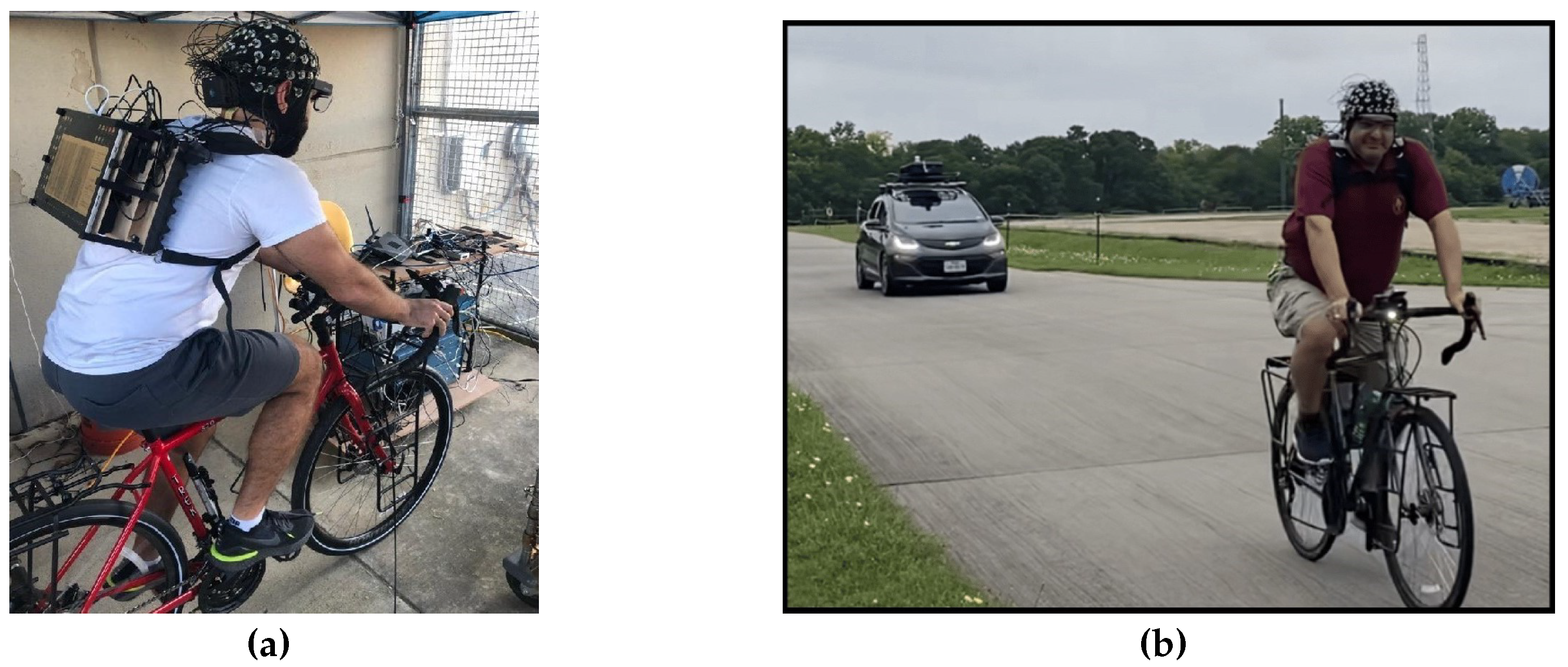
Figure 1 shows the experimental setup scenario for simultaneous measurement of biometric variables and environmental variables.
Two of the experimental paradigms in this study also share some similarities and differences.
Table 1 shows some of the similarities between the two experimental paradigms.
The differences between the two experimental paradigms is given in
Table 2.
2.2. Data collection
The process of data collection in both experimental paradigms involves simultaneous measurement of biometric data (or biometric variables or predictor variables) using the same biometric suite and the environmental data (or target variable or pollutant). Several biometric variables were measured, among which the ones that have been considered for the study are given in
Table 3:
The EEG data were collected using a Cognionics EEG headset consisting of 64 electrodes following the 10-10 nomenclature system [
47] (
https://www.cgxsystems.com/mobile-128, accessed on 16 January 2024) with a sampling rate of 500 Hz. Among the rest of the physiological responses (or non-EEG variables) the ECG, GSR,
, respiration rate, skin temperature, and heart rate were measured using the Cognionics AIM Generation 2 device (
https://www.cgxsystems.com/auxiliary-input-module-gen2, accessed on January 16, 2024) with a sampling rate of 500 Hz. The Tobii Pro Glasses 2 (
https://www.tobii.com/products/discontinued/tobii-pro-glasses-2, accessed 16 January 2024) gives several pupillometric measurements at a sampling rate of 100 Hz but the ones that have been considered are the pupil diameter of the left eye, pupil diameter of the right eye, and distance between the pupils.
The data obtained from each of the 64 electrodes ( or channels) of the EEG headset is received as a time series of voltage. These voltages are with respect to a virtual reference that is averaged from all the channels. The voltage time series can be transformed from the time domain to the frequency domain. One of the ways to do so is the Welch method [
48] which was implemented using scipy [
49]. The transformation thus gives a power spectrum density (
) in the Y axis and a frequency in the X axis. The frequency can be divided into five frequency bands named delta, theta, alpha, beta, and gamma, each representing a different brain state. With the data obtained from each of the 64 electrodes, transforming each into a frequency domain and dividing each frequency into five frequency bands provides a total of 320 biometric variables from the EEG headset.
From the three measured pupillometric variables, other variables such as the average pupil diameter of the two pupils, the difference between pupil diameters of the left and right eyes, and the absolute value of the difference between the pupil diameters, giving extra features to be considered.
Before data collection for the study began, in each of the experiments, baseline biometric measurements were made for two minutes with the participants’ eyes closed and the eyes open. The biometric suite was placed in such a way as to have little effect on physiological responses.
At times, the precision of the data captured by biometric sensors can be compromised due to their movement, resulting in the possibility of no values being recorded. Furthermore, the devices also have different sampling rates. Therefore, the data were cleaned and down-sampled to 1 second for CO
2, 5 second for NO
2, 5 second for NO, and 1 second for
. The total number of biometric variables used and the number of data records collected for each pollutant are given in
Table 4.
Data collection of CO2, NO2 and NO was carried out on three separate days: On 26 May, 9 June, and 10 June 2021, accurate data for CO2 reading were received only on 9 June 2021 and 10 June 2021 with 2 trials on each day. Accurate data for NO2 and NO were received on all 3 days with 2 trials on each day. Data collection for PM1 and PM2.5 took place on October 21 2021, January 14 2022, January 27 2022, and February 9 2022 with different participants on each day.
Data obtained for NO2 and NO from the measuring device were filtered to include only records that passed multiple quality criteria. These quality criteria included (a) the cell flow rate of the sample gas to be (1400 to 1600) cc/min, (b) the ozone flow rate to be (60 to 80) cc/min, (c) the cell photodiode voltage (PDV) to be at least 0.6 Volt, and (d) the PDV ozone generator to be at least 0.1 Volt.
2.3. Data analysis and developing machine learning model
After the construction of the four datasets consisting of biometric variables as the input features, and the output target variables we sought to estimate being the inhaled pollutant concentrations. Each target variable was estimated separately using Random Forests [
50] for multidimensional nonlinear regression using the ensemble Random Forest Regressor package from scikit-learn [
51]. All models were trained using 80% of the data, and the remaining 20% was used as an independent test set. The determination coefficient (r
2) and the root mean square error (RMSE) are calculated between the true values of the pollutant and the estimated values of the pollutant to quantify the goodness of fit. Scatter plots, quantile-quantile plots, and time series plots of the actual and estimated pollutant values have also been plotted for a qualitative analysis of goodness of fit.
Each of the scatter diagrams has the true values of the pollutant on the X axis and predicted values on the Y axis. In each of the scatter diagrams, the data points in the testing test are denoted by an orange "x" sign, whereas the data points in the training set are denoted by filled blue circles. A 1:1 black line has been overlaid in the scatter diagram to indicate how far the prediction is from the true values with data points with an exact prediction lying on the 1:1 line. A quantile-quantile plot for each of the four machine learning models has been drawn and overlaid with percentiles to indicate where in the distribution the data points deviate from the actual values with data points that have an exact prediction lying on the red 1:1 line.
To identify the effectiveness of biometric variables in predicting the target variable, the SHAP values (SHapley Additive exPlanations) [
52,
53] of the SHAP library were used to rank the predictor variables in descending order. The SHAP values for variables below the ninth order were found to be small and thus less effective in making the prediction. Since the data are mostly nonlinear, the top 9 of those variables in the predictor ranking were then used, and a 10 by 10 mutual information matrix including the pollutant to be estimated was calculated using a package from sckit-learn [
51] to identify the nonlinear relationship between the variables. These mutual information values are greater than zero, with higher values indicating a stronger relationship, and zero values indicating that the two variables are independent of each other.
3. Results
Among the several biometric variables that have been measured in this study, some of the readings are not easily measurable and the devices are expensive as well, for example, EEG, Tobii Pro glasses 2. Other variables such as skin temperature, , heart rate, respiration rate, GSR, and ECG can be measured relatively easily and are also inexpensive. Therefore, the study is classified into two parts; first, we consider all biometric features that have been measured, and second, we consider biometric variables that can be easily measured and accessible.
3.1. Using all features
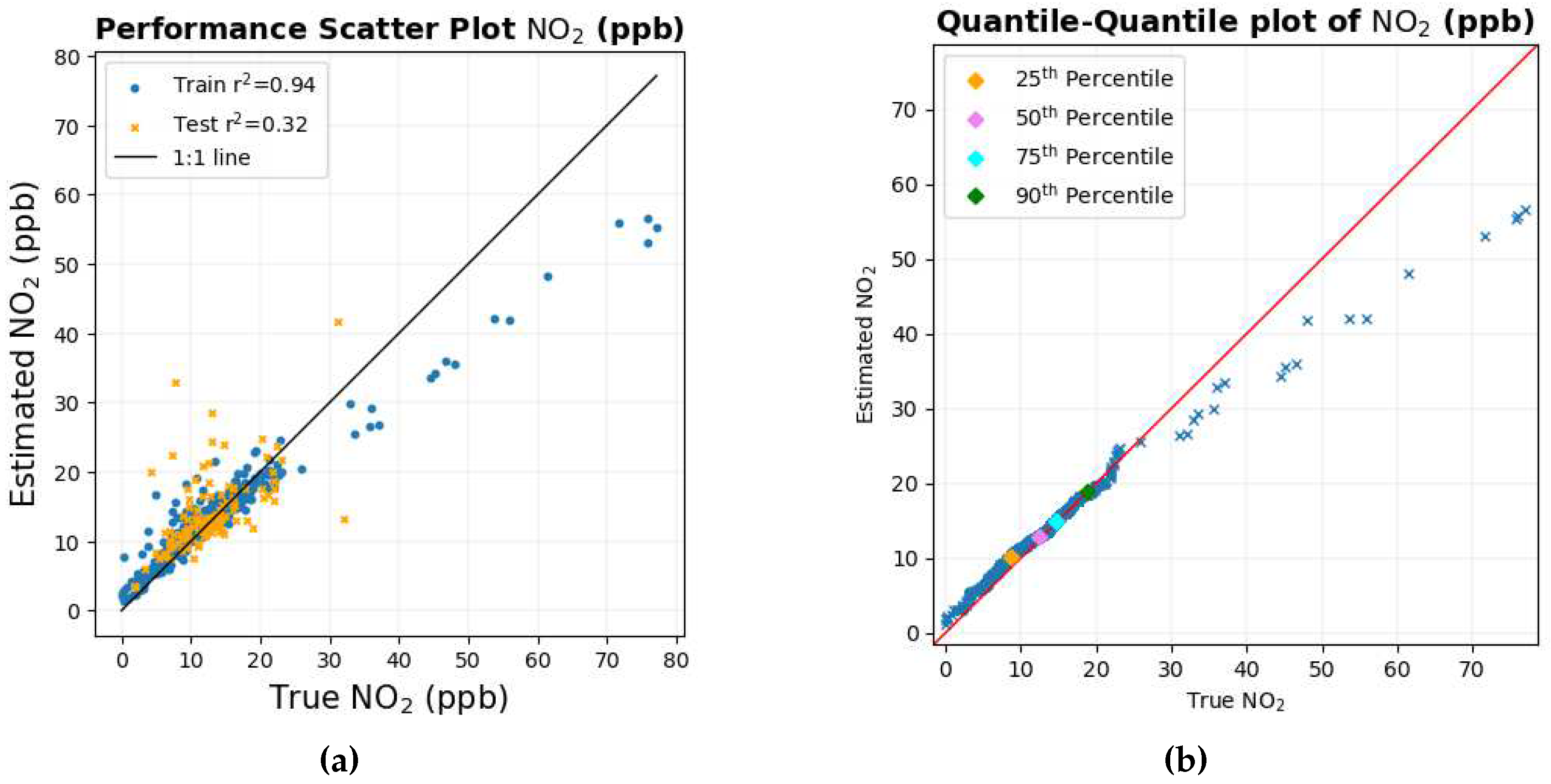
Table 5 shows the coefficient of determination (r
2) and RMSE between the true values of the pollutant and the estimated values of the pollutant in the training set and the testing set for each pollutant using the Ensemble Random Forest Regressor package from scikit-learn considering all biometric variables. As the dataset in this case consists of large number of features, hyperparameters of the random forest model have not been optimized as it was time consuming; thus default parameters have been used.
Table 5 shows that the train r
2 for all pollutants is nearly 1 and the train RMSE is also low, which is expected since this part of the data set is used by the machine learning model for learning. The independent test r
2 for PM
1, CO
2 and PM
2.5 is also almost 1, and the RMSE is also small, indicating that the performance and generalization of the machine learning model in estimating PM
1, CO
2 and PM
2.5 is very good. For pollutants such as NO
2 and NO, for which we had far fewer data records, the performance was not as good, with low test r
2 values. One possible explanation for the result is that there are not enough training examples, as shown by the scatter diagram in
Figure 5a and
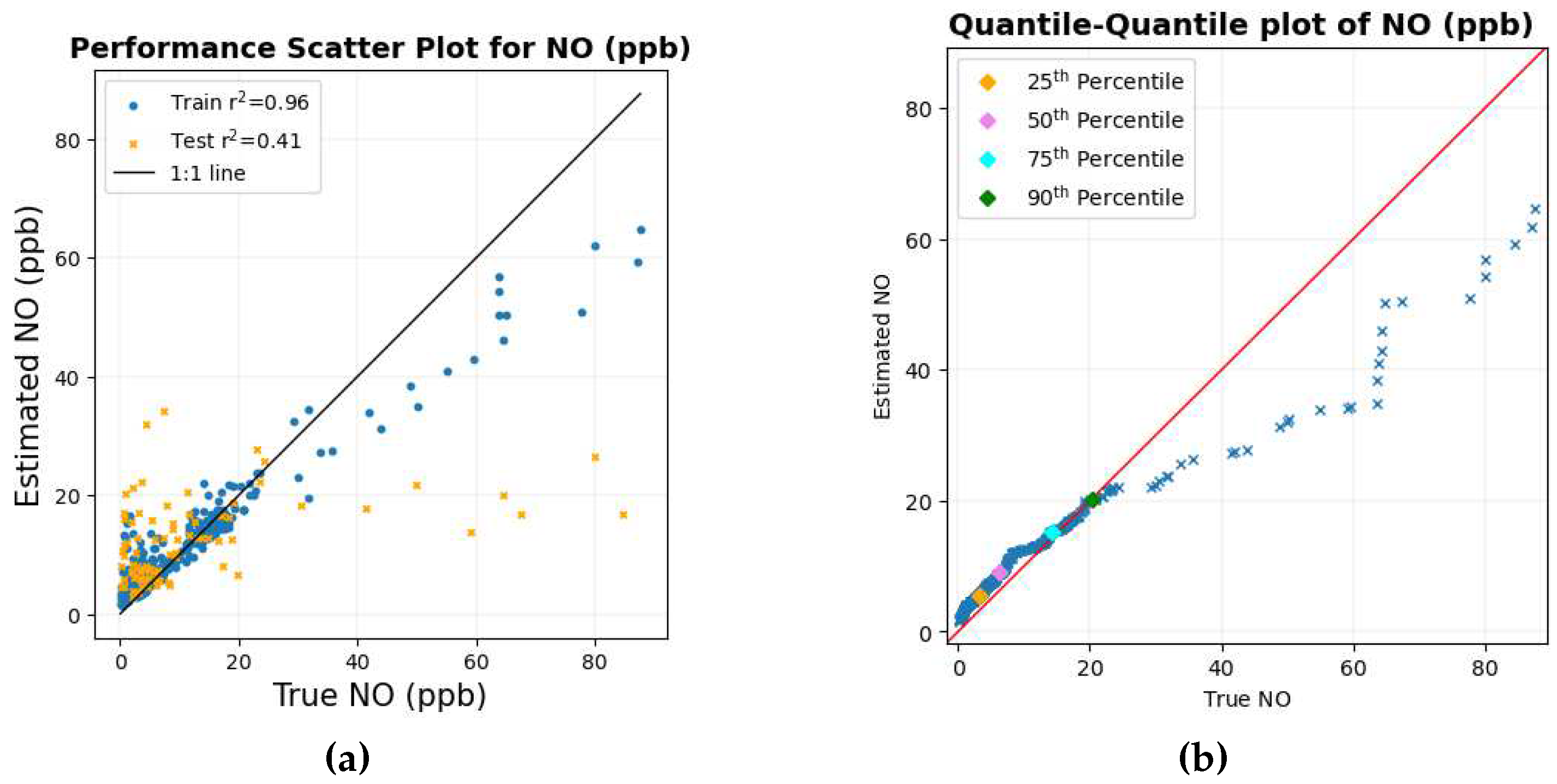
Figure 7a. The r
2 values and the RMSE values for all these pollutants can change according to the way the data is shuffled. For PM
1, PM
2.5 and CO
2 these values remain close to each other because there is an abundance of data points over a range of values. However, for NO
2 and NO, these values change to some extent depending on how the data are shuffled, especially considering the large number of predictor variables for a relatively small data set. When the algorithm was run five times, the average r
2 in the training set and the NO
2 test set was 0.91 and 0.14, respectively, and the average RMSE was 3.21 ppb and 7.86 ppb in the training set and test set, respectively. Similarly, for NO, when the algorithm was run five times, the average r
2 value in the training and testing set was 0.93 and 0.19, respectively, and the average RMSE was 5.07 and 14.75 ppb, respectively.
3.1.1. Carbon dioxide
For the study of CO
2 a total of 329 biometric input variables were taken into account, including the 320 variables from the EEG data, and the remaining variables include: ECG, respiration rate, SpO
2, heart rate, GSR, skin temperature, pupil distance, average pupil diameter and absolute value of the difference between pupil diameter.
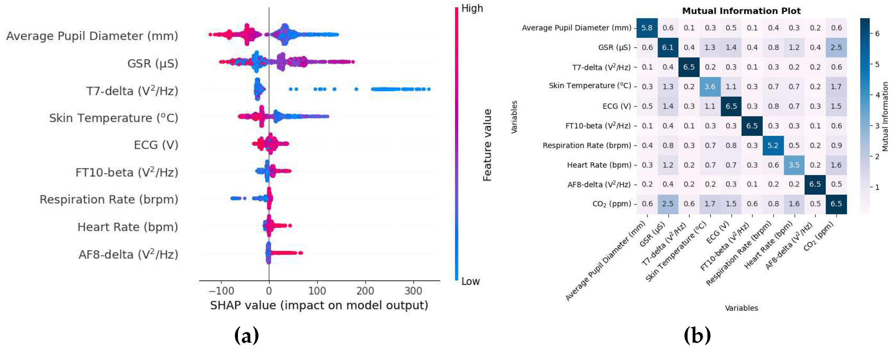
Figure 2a shows a SHAP value beeswarm plot of the top 9 features in descending order to indicate the biometric variables that were the most influential in estimating CO
2.
Figure 2b shows a mutual information matrix consisting of the 9 variables with the 9 highest SHAP values and CO
2.
These SHAP values for CO2 on the X axis are expressed in units of ppm. As indicated by SHAP values, the average diameter of the pupil, the GSR and skin temperature are among the top physiological responses that were the most effective in predicting CO2. The order of these variables can change depending on how the data are shuffled, especially when the SHAP values are close to each other, for example, features in order numbers 5,6 and 7. The plot also indicates that higher values of the average pupil diameter tend to decrease the prediction, while lower values tend to increase the prediction as large portions of SHAP values for the average pupil diameter are negative and positive, respectively.
In addition to the fact that the diameter of the pupil changes depending on the light entering it, the diameter of the pupil has been associated with cognitive ability [
54]; as mentioned before CO
2 intake is linked to cognitive issues [
30,
31,
32] as well. The GSR sensor measures the response to sweat, and sweating can be caused by physical tasks such as cycling. CO
2 inhalation can cause sweating when the concentration is 6 to 10% [
55]. Other biometric variables include respiration rate, heart rate, skin temperature, and considering that exposure to CO
2 can cause physiological changes in lung and cardiovascular function [
33], it is expected that these variables will be affected by CO
2 intake.
Similarly, the EEG variables included T7, FT10, and AF8 electrodes with frequency band delta, beta, and delta bands, respectively. According to the system of nomenclature 10-10 [
47], electrodes with odd numbers are on the left side and those with even numbers are on the right side. T7 electrode is above the temporal lobe, which is associated with speech and short-term memory [
56]. The FT10 electrode is located between the frontal and temporal lobes. The SHAP value of the AF8 electrode is very small, and therefore all variables below the order have a smaller SHAP value and provide a small contribution in CO
2 prediction.
The mutual information matrix shows that inhaling CO2 has a high nonlinear relationship with GSR, skin temperature, ECG, respiration rate, and heart rate indicating the several changes brought about by CO2 intake. Similarly, these biometrics are also mutually related with each other as GSR as high mutual information with average pupil diameter, skin temperature, ECG, heart rate; skin temperature with ECG, ECG with respiration rate; respiration rate with heart rate.
The scatter diagram and the quantile-quantile plot for CO
2 are shown in
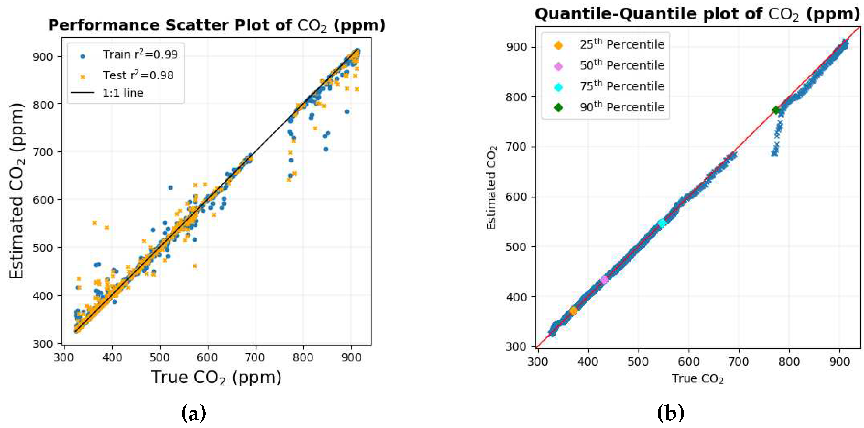
Figure 3. The scatter diagram in
Figure 3a shows that most of the data points in the training set but, more importantly, in the testing set lie very close to the black 1:1 line, indicating that the predictions are close to each other for most of the data set. The quantile-quantile plot in
Figure 3b also shows that for most of the distribution, the data points lie close to the red 1:1 line. The quantiles in the distribution deviate for values between 700 and 800 ppm, and one of the possible reasons could be the scarcity of data points in this range of value, which is also depicted in the scatter diagram.
3.1.2. Nitrogen dioxide
The 329 variables that have been considered for the study of NO
2 include the 320 EEG variables, ECG, respiration rate, SpO
2, heart rate, GSR, skin temperature, average pupil diameter, pupil distance and difference in pupil diameter. In the case of NO
2, the estimate was not as good, as indicated by the value of r
2 and RMSE between the true and estimated values of NO
2 in
Table 5. However,
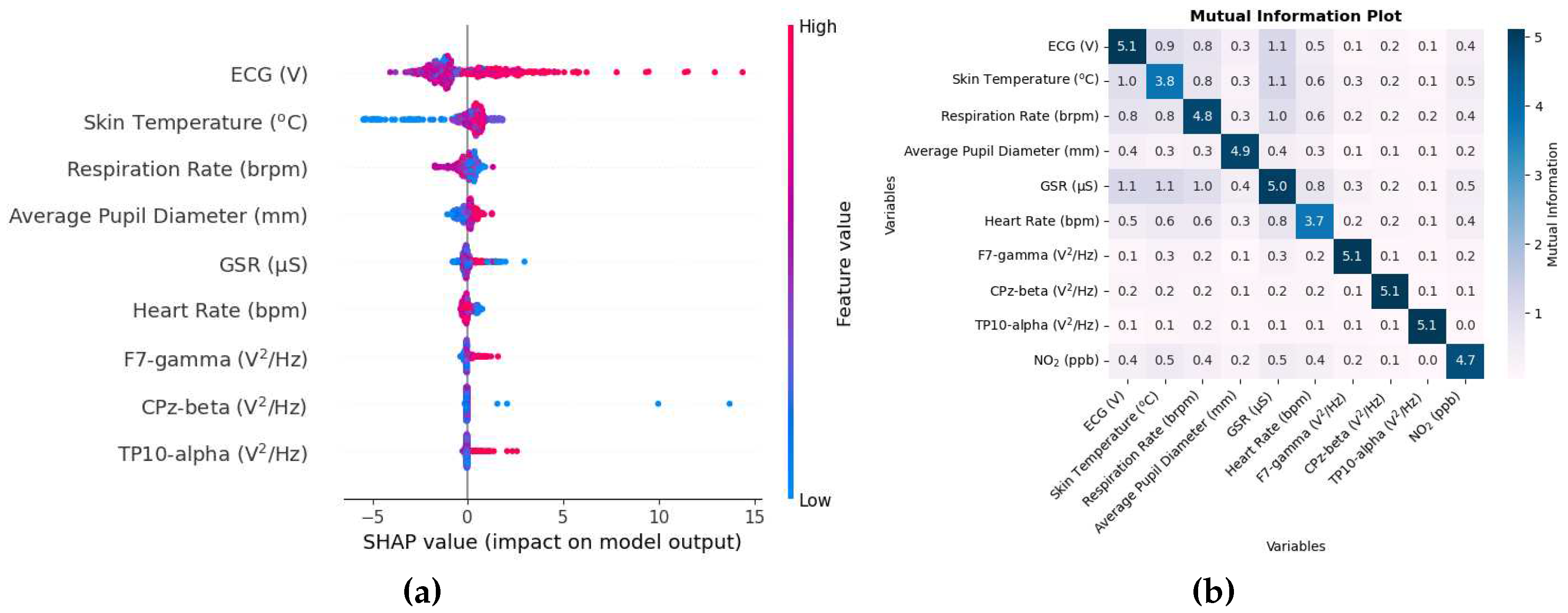
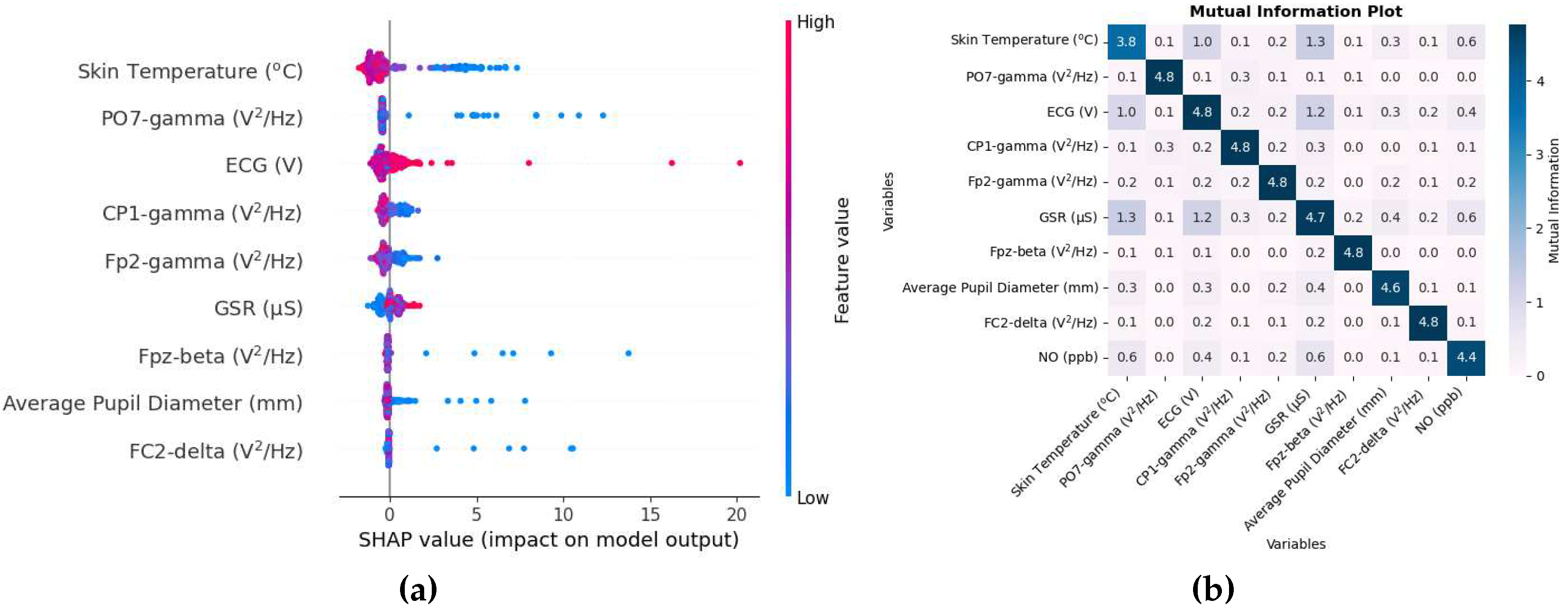
Figure 4a shows the SHAP value beeswarm plot of the top 9 biometric features that were most influential in estimating NO
2.
Figure 4b shows the mutual information matrix of the top 9 features chosen by SHAP values and NO
2.
The SHAP values in this case on the x-axis are in units of ppb. The SHAP value of the ECG and skin temperature is relatively higher than other variables, so these variables do not tend to change order. However, the ordering of the rest of the variables can change depending on how the data are shuffled, as the SHAP values are close to each other, especially at the lower end of the order. The plot also shows that lower values of skin temperature tend to decrease the prediction, while higher values tend to increase the prediction. As long- and short-term exposure to NO
2 has been associated with cardiovascular disease [
57], it is likely that the ECG is one of the main variables. As inhalation of a higher concentration of NO
2 causes inflammation of the airways, changes in respiration rate, skin temperature, and sweating are also likely to affect the GSR sensor.
Other variables include EEG ones. F7 electrode is one of the main EEG variables. The SHAP value of the F7-gamma variable and the following two variables are small compared to the rest of the other variables, indicating their small effectiveness in estimating NO2.
The mutual information matrix in
Figure 4b shows that NO
2 has high mutual information with ECG, skin temperature, heart rate and GSR, again to be expected, as the SHAP values for these variables were high. The matrix also shows that the ECG has higher mutual information with skin temperature, respiration rate, heart rate, GSR; skin temperature with respiration rate, heart rate, GSR; respiration rate with heart rate, GSR; heart rate with GSR. This is similar to what is seen in the mutual information matrix in
Figure 2b indicating that the variables are mutually related to each other.
The scatter plot and the Quantile-Quantile plot for NO
2 are shown in
Figure 5a and
Figure 5b, respectively. The scatter diagram in
Figure 5a shows that the lower values of the data points lie close to the black 1:1 line where there is an abundance of data. The Quantile-Quantile graph in
Figure 5b shows that around 90% of the data is less than 20 ppb where the Quantile-Quantile graph is close to the red 1:1 line. As the values of NO
2 increase, the number of data points is scarce; this could possibly have caused the number of data points to deviate from the 1:1 black and red line for higher NO
2 values, as there is a very small number of data points from which the machine learning model can learn.
3.1.3. For NO
In the NO study, the same 329 variables used in NO
2 were considered. Similarly to the case of NO
2, the estimation of NO using biometrics does not appear to be very accurate, as indicated by r
2 and the RMSE values between the true and estimated values of NO in
Table 5, a possible explanation can be given by the scatter plot and the Quantile-Quantile plot in
Figure 7.
The unit of SHAP value on the x-axis here is ppb. The SHAP value beeswarm plot in
Figure 6a shows that physiological responses such as skin temperature, mean pupil diameter, and ECG are among the main biometric variables in estimating NO. The plot also shows that higher values of skin temperature tend to lower the prediction, while lower values tend to increase the prediction. Since inhalation of NO when reacted with oxygen can create NO
2, skin temperature and ECG were possibly affected, which were also common variables in NO
2. There appear to be a large number of EEG variables as well. The PO7 electrode is located between the parietal and occipital lobes on the left side of the brain. The gamma band that seems common is dominant in tasks that involve concentration [
58]. Other biometric variables such as Fp2-gamma, Fpz-beta, and below them have small SHAP values and thus provide less contribution in NO estimation.
The mutual information matrix in
Figure 6b shows that among the predictor variable, NO has high mutual information with skin temperature and ECG; skin temperature and ECG have high mutual information with each other.
Figure 7 shows the scatter plot and the quantile-quantile plot of the true values of NO compared to the estimated values of NO.
The overall structure of the scatter diagram and the quantile-quantile graph for NO looks similar to that of NO
2, with smaller values of NO lying close to the corresponding 1:1 line where there is an abundance of data points. The Quantile-Quantile plot in
Figure 7b shows that more than 90% of the data are below around 20 ppb. As the values of NO get larger, these data points tend to deviate from the 1:1 line; one of the possible reasons can be attributed to the scarcity of data points in the region.
3.1.4. PM1
Since in the static bike ride experimental setup where the measurement of PM
1 and PM
2.5 was performed, the T7 electrode of the EEG headset did not give any readings, the number of biometric variables was reduced to 322. These biometric variables include the 315 variables of the EEG headset, respiration rate, SpO
2, heart rate, skin temperature, average pupil diameter, pupil distance, and difference in pupil diameter. As shown in
Table 5, PM
1 performance was the highest with r
2 value of 0.99 and the lowest RMSE of 0.06
g/m
3 in the test set.
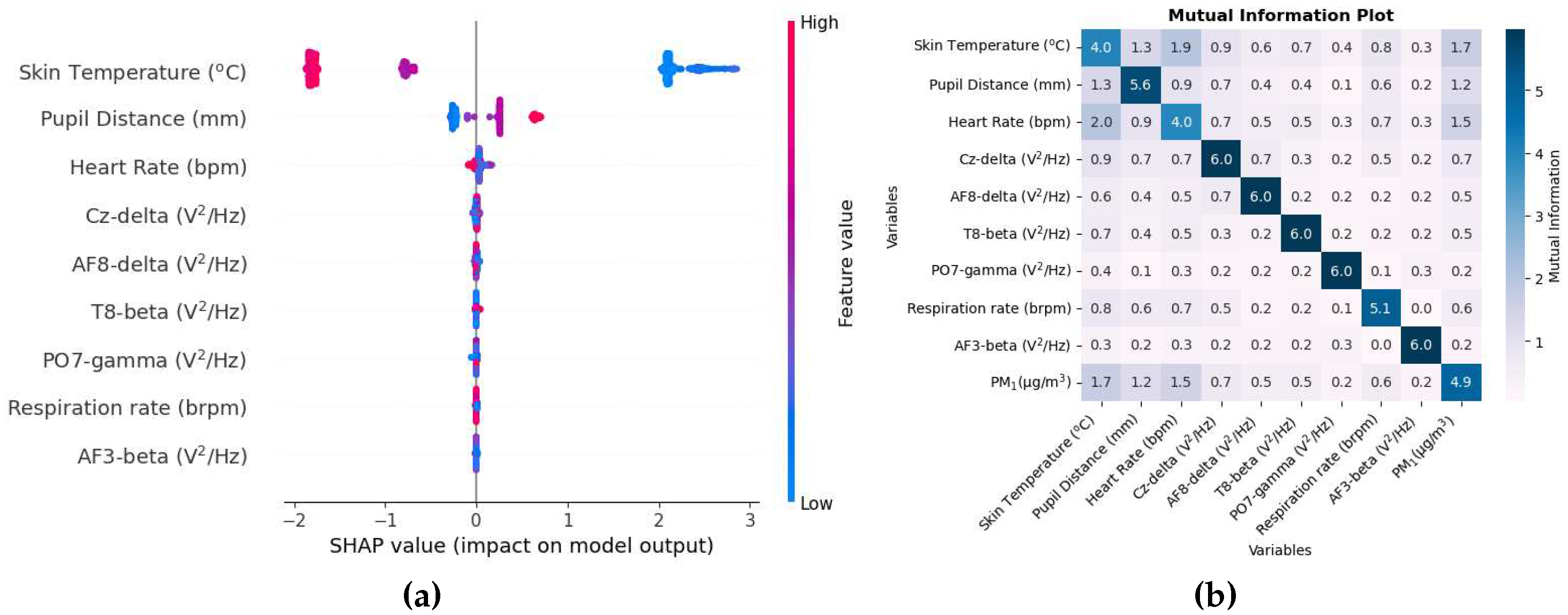
The SHAP value beeswarm plot in
Figure 8a shows that skin temperature, pupil distance, and heart rate are among the main features that were the most influential in estimating PM
1. The skin temperature and the distance of the pupil were also important variables in the estimation of PM
1 when a single participant was used for the study [
46]. The distance of the pupils, which indicates vergence of the eyes, has been associated with attention load [
59]. A series of EEG variables are amongst the top variables where the SHAP value of the Cz-delta variable is small and all the variables below it are even smaller, which is very close to zero. Thus, removing these features in the study will have little effect in estimating PM
1.
The mutual information matrix in
Figure 8b shows that PM
1 has high mutual information with physiological responses such as pupil distance, heart rate, respiration rate, and also shows that the physiological responses are indeed mutually related with each other.
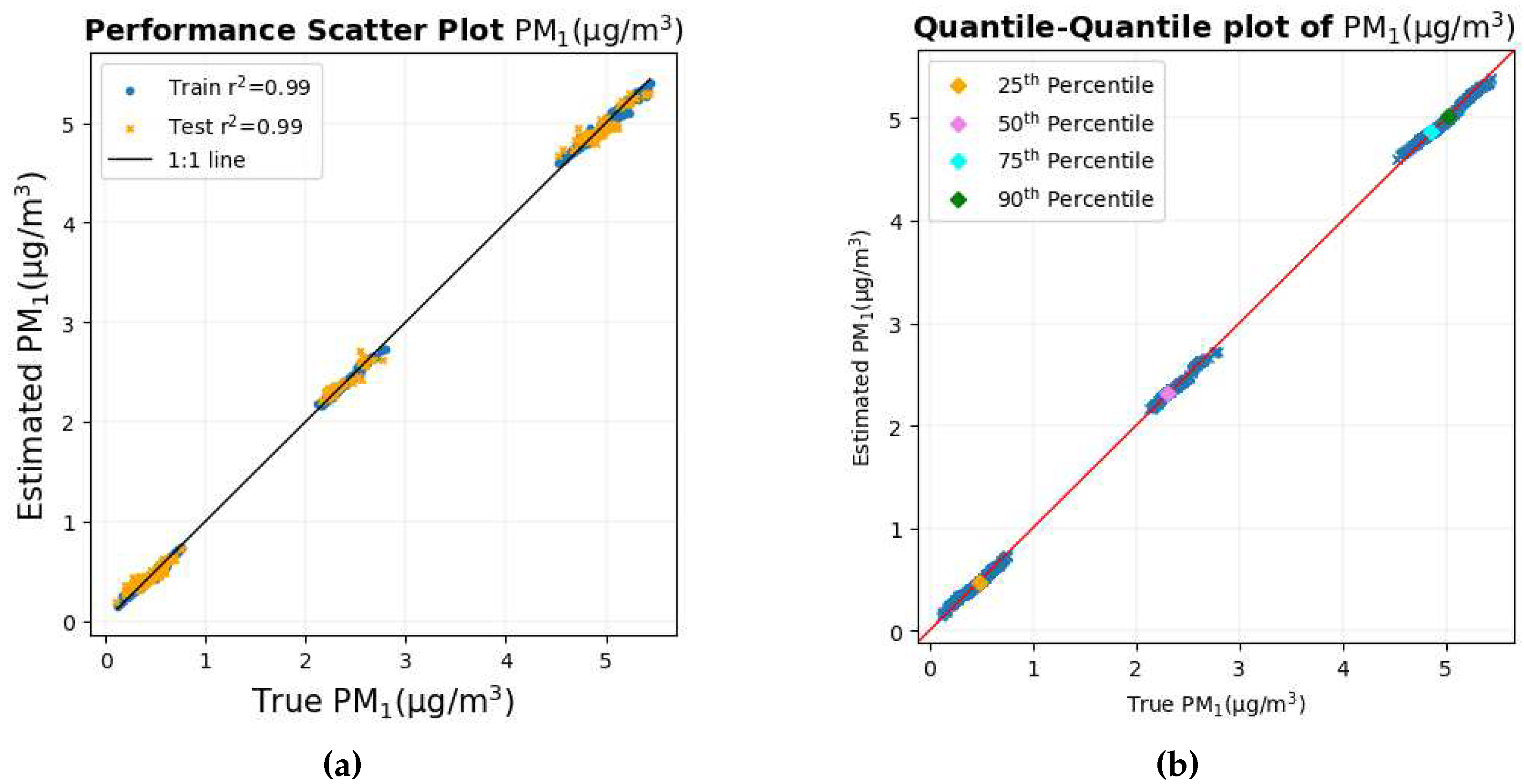
The scatter diagram and quantile-quantile graph with true PM
1 values on the X axis and estimated PM
1 values on the Y axis are shown in
Figure 9a and
Figure 9b, respectively.
Both the scatter plot and the quantile-quantile plot show that the data points are very close to the 1:1 line of the corresponding graph, indicating that the prediction is the most accurate and precise among all the pollutants.
3.1.5. PM2.5
The biometric variables that have been considered in the study of PM
2.5 are the same as those of PM
1. As shown in
Table 5, the estimation of PM
2.5 was highly accurate, as indicated by r
2 value between the true and estimated values of PM
2.5 in both the training and the test set, which is almost 1. The RMSE is also the lowest among all pollutants.
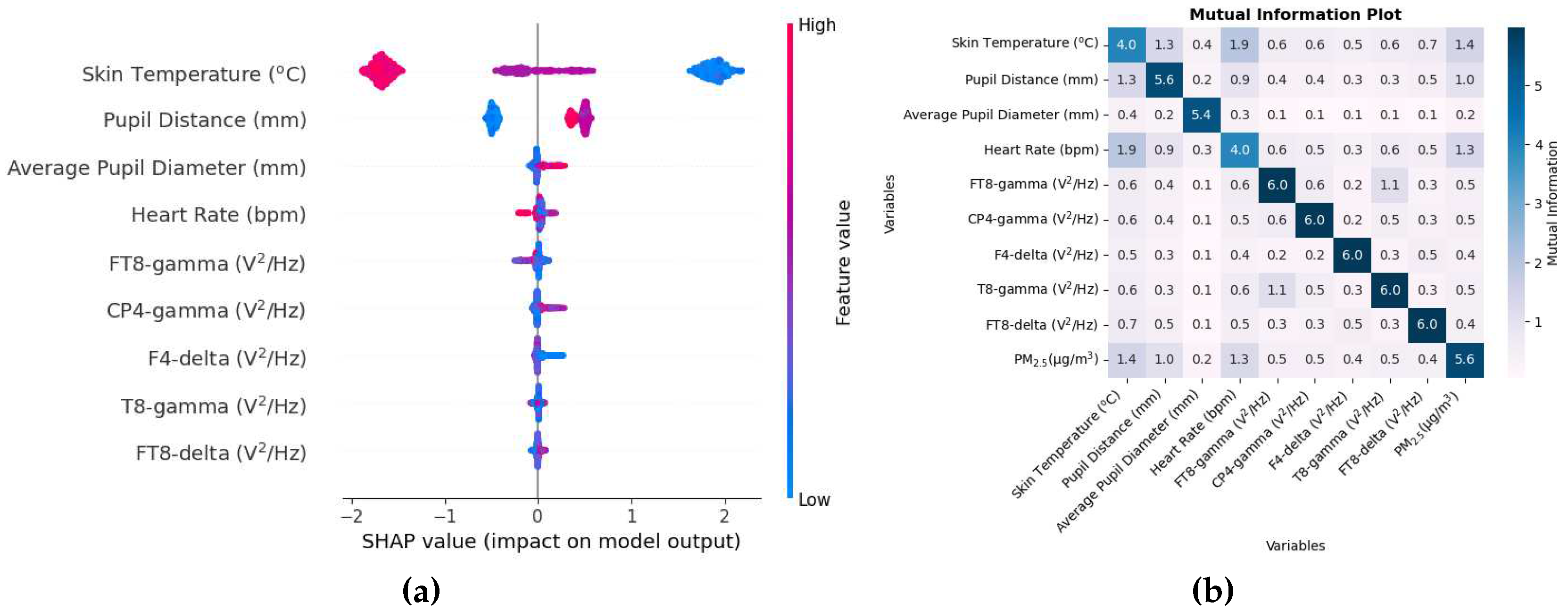
The SHAP value beeswarm plot in
Figure 10a shows that the physiological responses that were the most effective in estimating PM
2.5 include skin temperature, pupil distance, average pupil diameter, and heart rate, three of which are common to that of PM
1. The SHAP values in the x-axis here is
g/m
3. The inflammatory response created by the higher concentration of PM
2.5 can possibly cause changes in skin temperature and heart rate. Furthermore, PM
2.5 also causes adverse health effects on the respiratory system [
3] and heart problems [
5] could be the reason why heart rate is one of the most important variables. The size of the pupils has been associated with cognitive ability [
54].
Several EEG variables are on the list of the top 9 variables. The FT8 electrode is located on the right side of the brain between the frontal and temporal lobe. The CP4-gamma variable has a small SHAP value with variables below the order of even smaller SHAP values, indicating that the elimination of these variables will have little effect on the prediction of PM2.5.
The mutual information matrix in
Figure 10b shows that there is some sort of non-linear relationship between PM
2.5 and skin temperature, pupil distance, and heart rate, again to be expected, as the SHAP values for these variables were also high. Just as in the case of other pollutants where physiological changes were related to each other, so is the case here as well with skin temperature, pupil distance, and heart rate mutually related to each other.
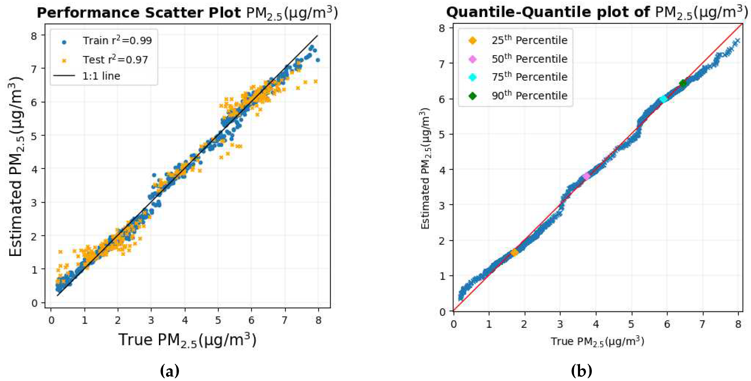
Figure 11a and
Figure 11b show the scatter plot and the quantile-quantile plot of the true values of PM
2.5 versus the estimated values of PM
2.5.
The scatter plot and the Quantile-Quantile plot in
Figure 11a and
Figure 11b, respectively, show that most of the data points lie in the 1:1 line of the corresponding graph. This shows that for most of the data set, the estimate is close to the true PM
2.5 values.
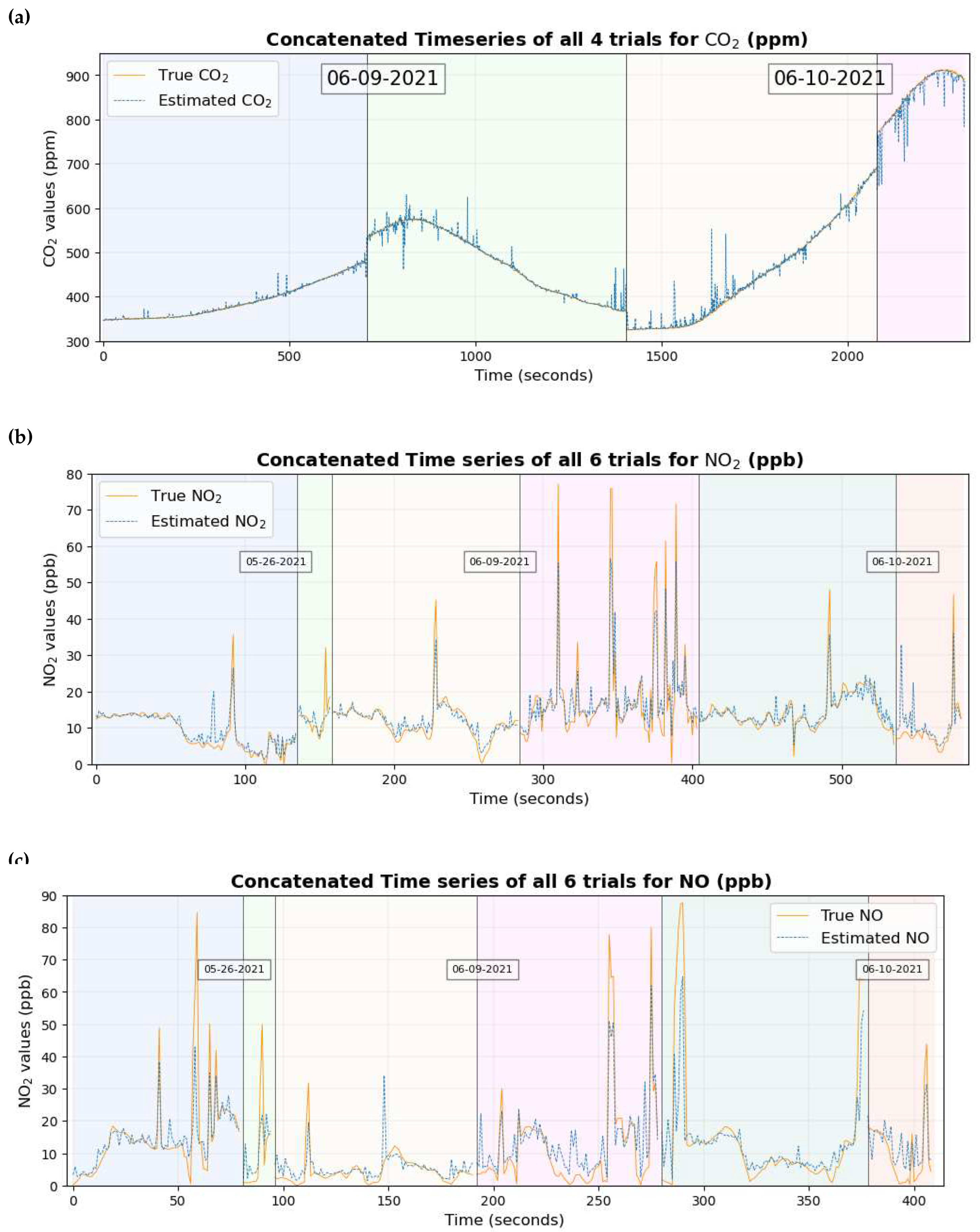
A time series graph of the 3 gaseous pollutants is shown in
Figure 12. Each of the time series plots includes true values in a continuous orange line and estimated values overlaid in dotted blue lines. The background has also been shaded with different colors depending on different trials and the trials have been separated by vertical black lines.
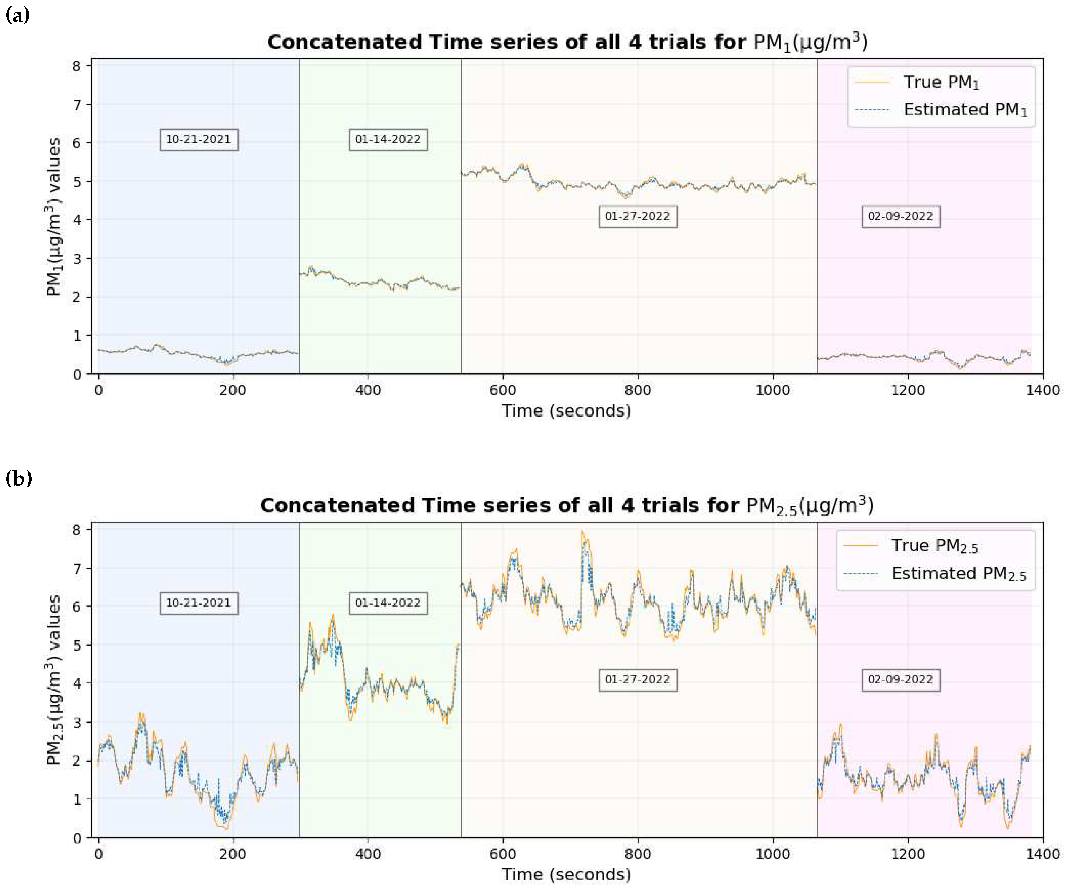
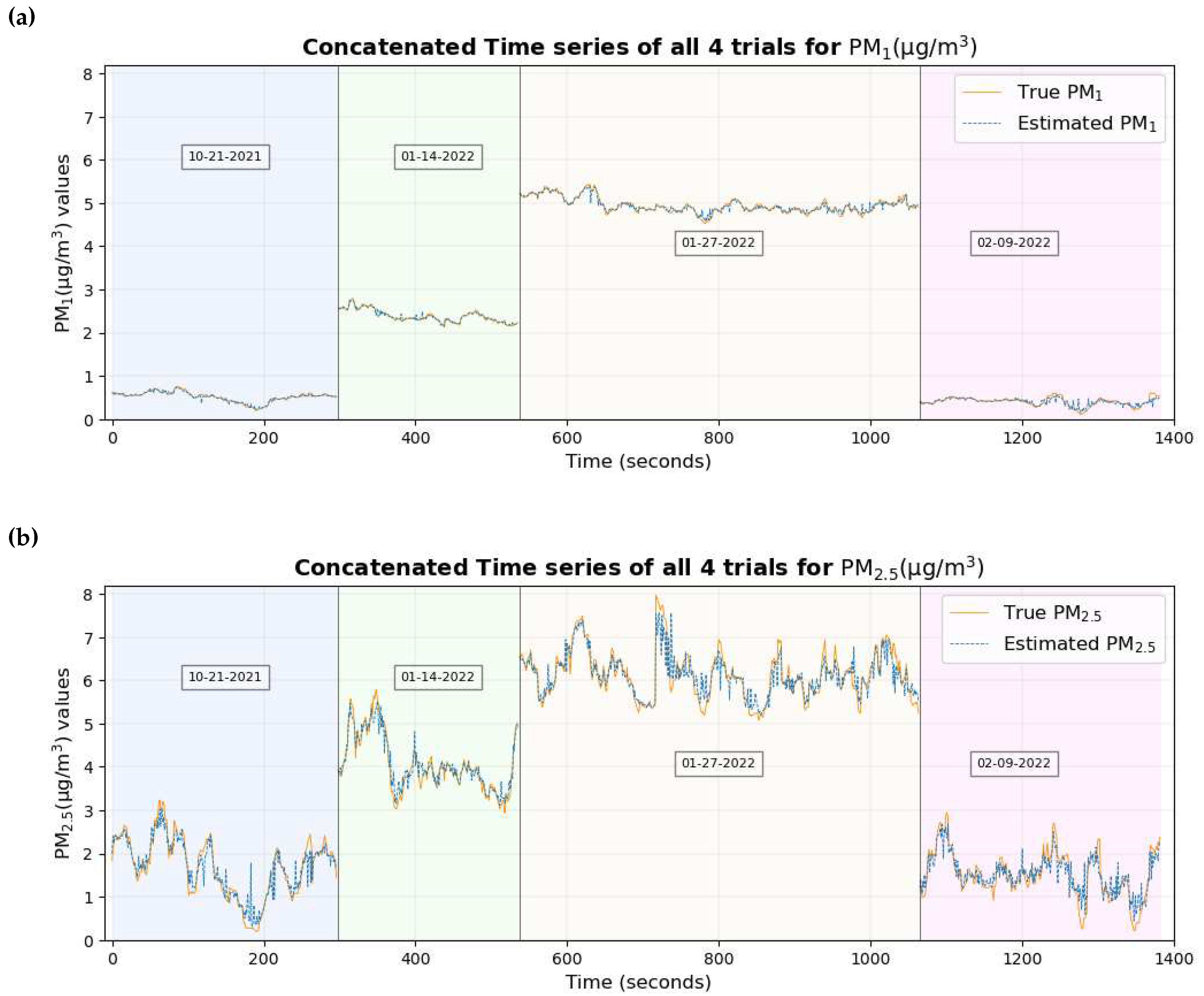
Figure 13 shows the time series plot of the true values of PM
1 and PM
2.5 overlaid with the estimated values of PM
1 and PM
2.5 respectively.
Figure 12 and
Figure 13 show that the true values of the pollutant are close to the estimated values of the pollutant for most of the data set.
3.2. Using easily measurable variables
Now, let us focus on just the subset of biometric variables that can be easily measured using affordable sensors, for example, respiration rate, SpO
2, heart rate, GSR, skin temperature. All models using the reduced number of input features have been trained with the same ensemble random forest regression algorithm from scikit-learn. Since the number of features in this case is small, the hyperparameters have also been optimized, as it is not time consuming.
Table 6 shows the results of r
2 and RMSE between the true values and the estimated values of the pollutant with the corresponding number of biometric variables used to estimate the pollutant.
The comparison of
Table 6 with
Table 5 shows that the test r
2 and RMSE for PM
1, PM
2.5 and CO
2 are very close to each other. Similar results can be seen for NO
2 and NO as well, where the test r
2 is better and the test RMSE is very close to each other. The numbers for NO
2 and NO can change to some extent based on how the data are shuffled, but with little disparity, since the number of dimensions has now been significantly reduced. When the algorithm was run five times, the average r
2 value in the train and the test for NO
2 was 0.91 and 0.26, respectively, while that of NO was 0.94 and 0.39 respectively. Similarly, when the algorithm was run 5 times, the average RMSE in the train and test set was 2.86 ppb and 6.30 ppb for NO
2 while that of NO was 3.87 ppb and 11.70 ppb, respectively. The mentioned values clearly indicate that the performance when the number of variables was reduced has increased for NO
2 and NO.
Biometric variables that have been considered for CO
2, NO
2 and NO now include GSR, skin temperature, respiration rate, heart rate, and SpO
2 while those for PM
1 and PM
2.5 include skin temperature, heart rate, respiration rate, and SpO
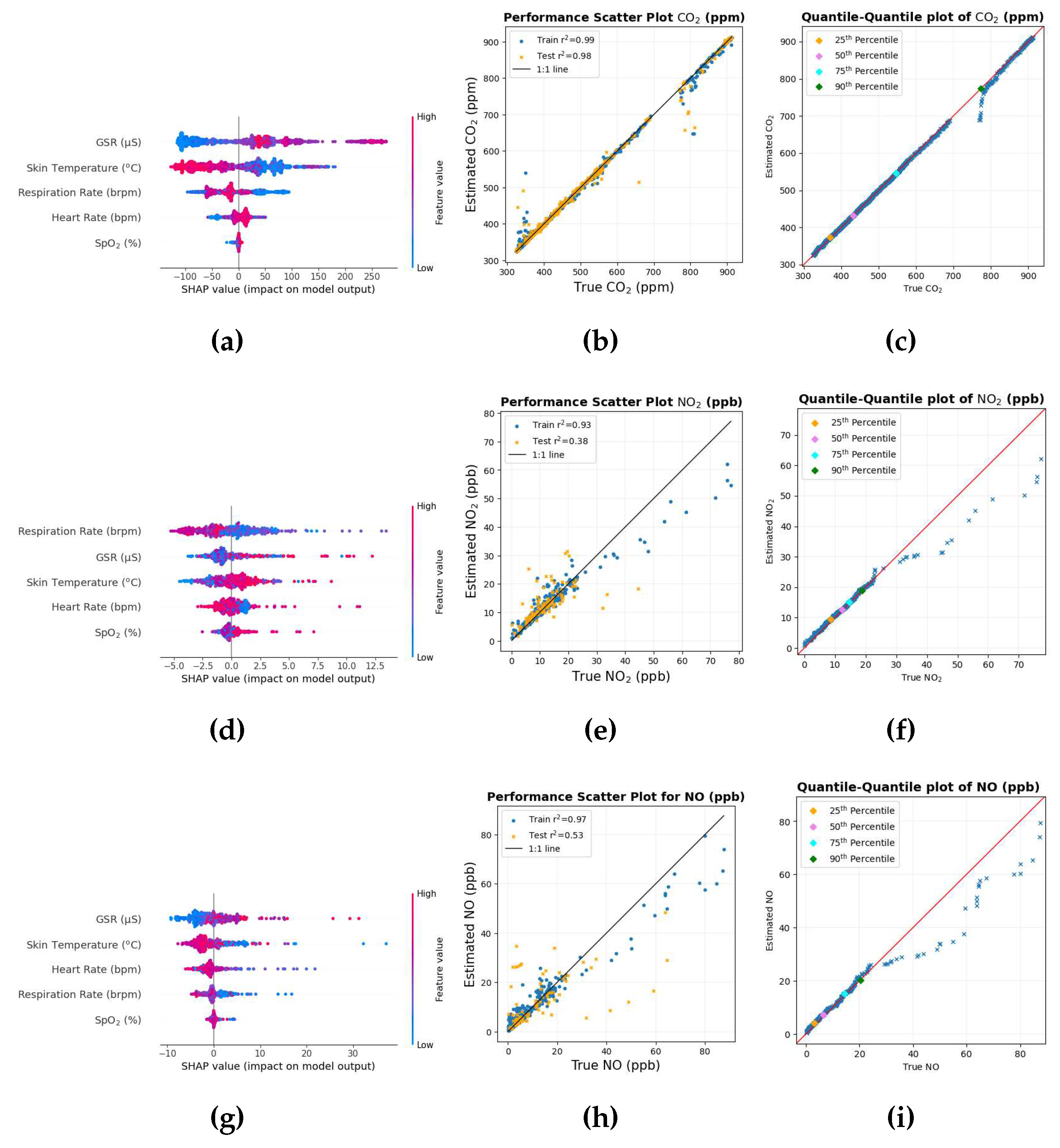
2. A SHAP value beeswarm plot, scatter plot and Quantile-Quantile plot of the gaseous pollutants estimated using the reduced number of variables is given in
Figure 14.
The ordering of the variables in the SHAP value is similar to each other for all gaseous pollutants. SpO2 seems to be the lowest among all pollutants and the elimination of this variable could have a small effect on the results. Since the number of dimensions has now been significantly reduced, the ordering will remain almost similar when the data is shuffled.
The scatter plot of CO2 is similar to that when all variables were considered. As the r2 value has increased for NO2 and NO, the data points in the scatter plot are closer to the 1:1 line.
Similarly, the structure of each Quantile-Quantile plot is similar for all gaseous pollutants when compared to the process in which all variables were considered.
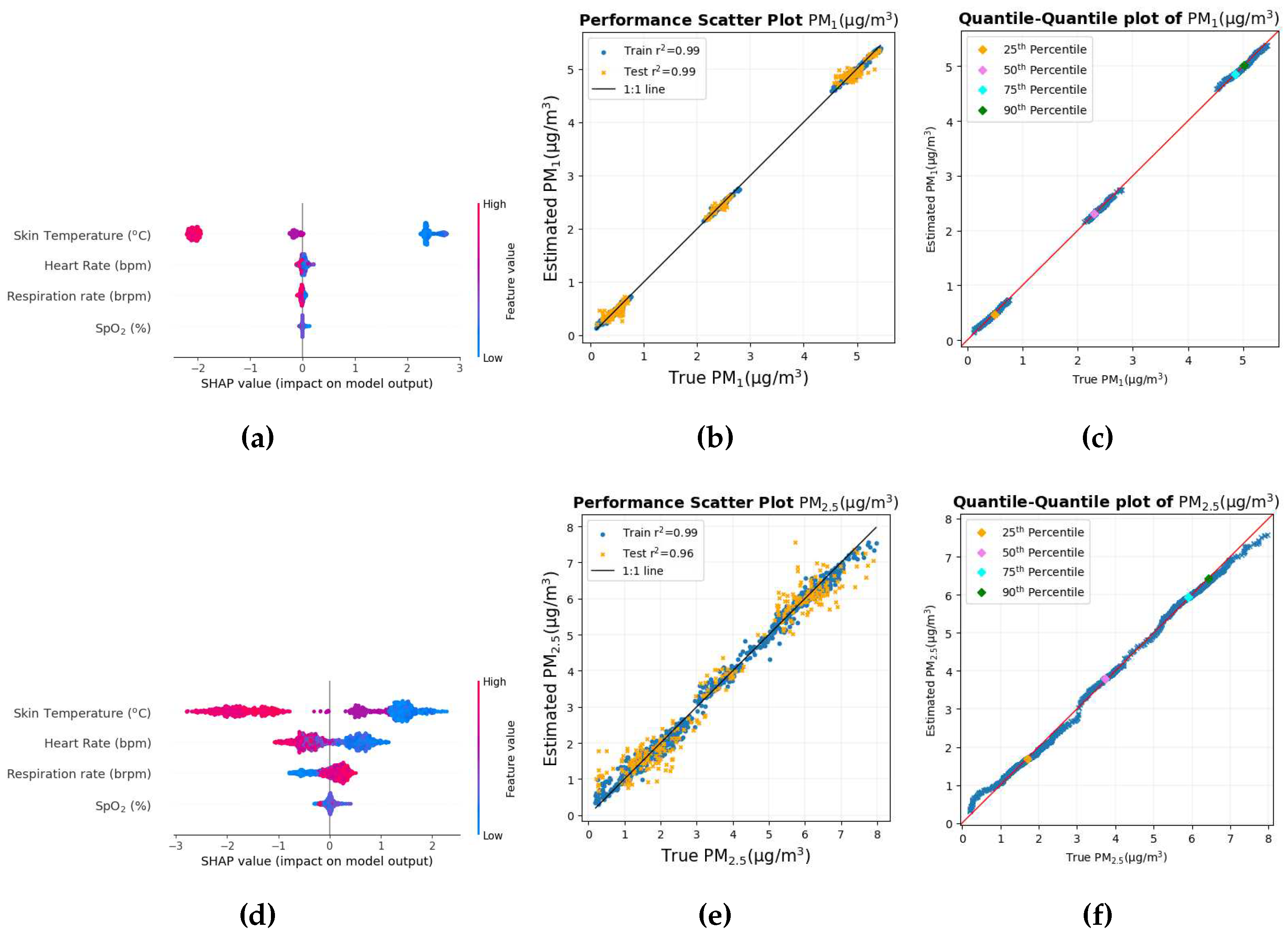
Figure 15 shows the SHAP value beeswarm plot, scatter plot and quantile-quantile plot when estimating PM
1 and PM
2.5 using only 4 biometric variables. The beeswarm plot in
Figure 15a and
Figure 15d shows that skin temperature remains the main variable for estimating PM
1 and PM
2.5 with a very high SHAP value compared to other variables. The overall structure of the scatter plot and the Quantile-Quantile plot of PM
1 and PM
2.5 also remains similar with a large portion of the data set close to the 1:1 black line and the 1:1 red line, respectively.
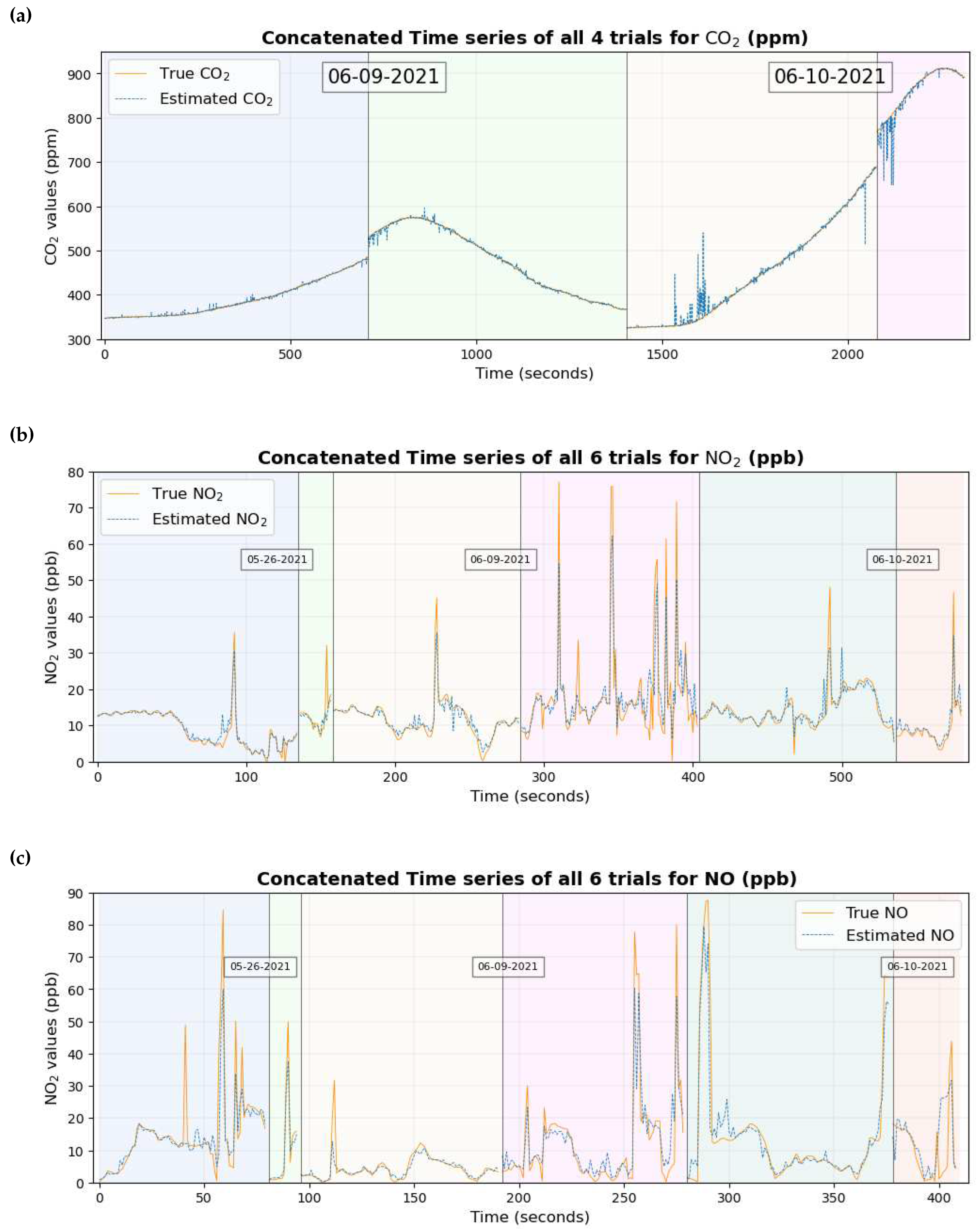
The time series plot with the reduced number of biometric variables to estimate CO
2, NO
2 and NO is shown in
Figure 16:
Figure 16a shows that the difference between the true values and the estimated values of CO
2 is now smaller, as the true values and estimated values are much closer to each other compared to the time series when all features were considered. Similarly, the time series plot for NO
2 and NO is also similar to that when all variables were considered.
The time series plot with reduced number of features to estimate PM
1 and PM
2.5 is shown in
Figure 17.
The time series plot of PM
1 and PM
in
Figure 17 shows that the true values and estimated values are close and are similar to those when all features were considered.
4. Discussion
The human body is a sensing system in itself and reacts to environmental variables and changes in them such as temperature, humidity, and air quality. It was previously shown that autonomous physiological and cognitive responses that result from the inhalation of particulate matter on a small temporal and spatial scale can be used to estimate PM
1 and PM
2.5 using machine learning models with very high accuracy [
46]; a study that was limited to a single participant. The inclusion of multiple participants in the experimental static bike ride paradigm where the measurement of PM
1 and PM
2.5 was performed shows that the methodology that was implemented on a single participant can be extended to multiple participants as well, producing even better results for PM
1 and PM
2.5 with a r
2 value of nearly 1 and a very low RMSE as shown in
Table 6. In fact, the results show that a few biometric variables are good enough to estimate PM
1 and PM
2.5 with similar results.
The time series plot of PM
1 and PM
2.5 in
Figure 17a and
Figure 17b shows that their true values are very close to the estimated values for the majority of the data set without any significant differences which explains their smallest RMSE among all pollutants. This supports the conclusion made previously [
46] that two of the possible reasons why these estimates are highly accurate and precise could be (a) these particulate matter are abundant and mix well with the ambient environment, thus having a higher probability of being inhaled by the participant and entering the sensors placed nearby (b) with the minute size of PM
2.5, these particulates, when inhaled, can reach deep into the lungs and bloodstream creating many negative health effects [
3,
5,
6], thereby impacting the human body to a large extent.
Air quality components include not only particulate matter, but also gaseous pollutants such as CO
2, NO
2, NO which have been included in this study. The methodology that was implemented to estimate and understand autonomous responses in the human body can be used for gaseous pollutants such as CO
2 as well. The r
2 value which is nearly 1 between the true and estimated values of CO
2 in the test set using a small number of biometrics supports this claim, as shown in
Table 6. Making the model simpler by considering a small number of biometrics also appears to have reduced the RMSE between the true and estimated values of CO
2 which can be seen clearly by comparing the time series in
Figure 13a and
Figure 16a.
The results to estimate NO
2 and NO for the entire range of data are not very accurate, as indicated by the value of r
2 and RMSE between the true and estimated values of the corresponding gas as shown in
Table 6. However, the scatter diagram of these two gases in
Figure 14e and
Figure 14h and the quantile-quantile plot of both of these gases in
Figure 14f and
Figure 14i indicate that the prediction is reliable to some extent for lower values of the gas where there is a higher concentration of data. As the number of data points decreases for higher values of these two gases, the data points in the scatter plot and the Quantile-Quantile plot deviate from their corresponding 1:1 line, with one possible reason being the very small number of data points for the machine learning model to learn from in this region of data. This could have possibly reduced the precision when the entire data set was considered for study. This claim is supported by the scatter diagram in
Figure 14b and the quantile-quantile plot in
Figure 14c of CO
2 where the data points deviate from the corresponding 1:1 line between 700 ppm and 800 ppm, one possible reason being the scarcity of data points in that region of data. Improvements in the result in future work can possibly be made by either large data collection or better machine learning models.
The result for all these air quality components shows that a small number of biometric variables used to estimate these pollutants provide similar and, in some cases, better results. This aligns with Occam’s razor principle that a simpler model usually generalizes well. Moreover, the reduction of the number of variables, that is, reducing the number of dimensions, was a necessity considering the small number of data sets compared to the large number of biometric variables that were collected.
There are a few limitations of this study that can possibly be removed in future work. One of them being the collection of data on a single participant for CO2, NO2 and NO. Multiple trials have been conducted to mitigate the issue. Future work can include a large number of data collection from multiple participants to provide further confirmation. The readings from some of the electrodes in the EEG headset can be distorted from activities such as blinks, head movement, swallowing, jaw clenching, neck movement, tongue movement, which is frequent when the participant is cycling. This results in a lot of noise in the data that can be removed, but these activities are frequent and the procedure can significantly reduce the number of data records. However, the results show that the removal of EEG data as biometric variables also yields similar results. The study can be done just by using a headset and observing how different areas of the brain can be affected when various components of air quality are inhaled.
The inclusion of confounding variables in the experimental setup is expected. Future work can also make use of the dataset and study the casual relationship among the variables.
Author Contributions
Methodology, D.L., S.T., T.L.; Software, S.R., S.T., B.F.; formal analysis, S.R., D.L.; data curation, S.T., D.L, L.W., B.F., T.L., M.L., J.S., A.A., J.W., P.H.; writing—original draft preparation, S.R.; writing—review and editing, S.R., D.L, J.W., L.W.; visualization, S.R.; supervision, D.L.
Funding
This research was funded by the following grants: The US Army (Dense Urban Environment Dosimetry for Actionable Information and Recording Exposure, U.S. Army Medical Research Acquisition Activity, BAA CDMRP Grant Log #BA170483). EPA 16th Annual P3 Awards Grant Number 83996501, entitled Machine Learning-Calculated Low-Cost Sensing. The Texas National Security Network Excellence Fund Award for Environmental Sensing Security Sentinels. SOFWERX Award for Machine Learning for Robotic Team and NSF Award OAC-2115094.
Institutional Review Board Statement
All experimental protocols were approved by The University of Texas at Dallas Institutional Review Board.
Informed Consent Statement
Informed consent was obtained from all the participants.
Data Availability Statement
Acknowledgments
The authors would like to acknowledge the OIT-Cyberinfrastructure Research Computing group at the University of Texas at Dallas and the TRECIS CC* Cyberteam (NSF 2019135) for providing HPC resources that were used in this study (
https://utdallas.edu/oit/departments/circ/.
Conflicts of Interest
The authors declare no conflict of interest.
Abbreviations
The following abbreviations are used in this manuscript:
| PM |
Particulate Matter |
| EEG |
Electroencephalogram |
| ECG |
Electrocardiogram |
| GSR |
Galvanic Skin Response |
| SpO2
|
Blood Oxygen Saturation |
| RMSE |
Root Mean Square Error |
References
- WHO. 7 million premature deaths annually linked to air pollution. http://www.who.int/mediacentre/news/releases/2014/air-pollution/en/, 2024. Accessed: 2016-08-29.
- U.S. Environmental Protection Agency. Air Quality Management Process, 2023. https://www.epa.gov/air-quality-management-process/managing-air-quality-air-pollutant-types, Last accessed on 2024-01-14.
- Xing, Y.F.; Xu, Y.H.; Shi, M.H.; Lian, Y.X. The impact of PM2. 5 on the human respiratory system. Journal of thoracic disease 2016, 8, E69.
- Franklin, M.; Koutrakis, P.; Schwartz, J. The role of particle composition on the association between PM2. 5 and mortality. Epidemiology (Cambridge, Mass.) 2008, 19, 680.
- Thangavel, P.; Park, D.; Lee, Y.C. Recent Insights into Particulate Matter (PM2.5)-Mediated Toxicity in Humans: An Overview. International Journal of Environmental Research and Public Health 2022, 19, 7511. [CrossRef]
- Kloog, I.; Melly, S.J.; Ridgway, W.L.; Coull, B.A.; Schwartz, J. Using new satellite based exposure methods to study the association between pregnancy PM2. 5 exposure, premature birth and birth weight in Massachusetts. Environmental Health 2012, 11, 1–8. [CrossRef]
- Li, Z.; Xiong, J. A dynamic inventory database for assessing age-, gender-, and route-specific chronic internal exposure to chemicals in support of human exposome research. Journal of environmental management 2023, 339, 117867. [CrossRef]
- Gu, Y.; Peach, J.T.; Warth, B. Sample preparation strategies for mass spectrometry analysis in human exposome research: Current status and future perspectives. TrAC Trends in Analytical Chemistry 2023. [CrossRef]
- Hartung, T. A call for a Human Exposome Project. ALTEX 2022, 40 1, 4–33. [CrossRef]
- Erdely, A.D. 157 Keynote: Understanding Exposure, Hazard Identification, and Human Health Effects: How Ultrafine/Nano Particle Toxicology Influenced Occupational Safety and Health. Annals of Work Exposures and Health 2023. [CrossRef]
- World Health Organization. Air Quality Guidelines. https://www.who.int/news/item/04-04-2022-billions-of-people-still-breathe-unhealthy-air-new-who-data, 2021. Guidelines for particulate matter (PM2.5 and PM10).
- United States Environmental Protection Agency. National Ambient Air Quality Standards (NAAQS) for Particulate Matter. https://www.epa.gov/pm-pollution/national-ambient-air-quality-standards-naaqs-pm, 2023. Standards for PM2.5 and PM10.
- Uwak, I.; Olson, N.; Fuentes, A.; Moriarty, M.; Pulczinski, J.; Lam, J.; Xu, X.; Taylor, B.D.; Taiwo, S.; Koehler, K.; others. Application of the navigation guide systematic review methodology to evaluate prenatal exposure to particulate matter air pollution and infant birth weight. Environment international 2021, 148, 106378.
- Block, M.L.; Calderon-Garciduenas, L. Air pollution: mechanisms of neuroinflammation and CNS disease. Trends in Neurosciences 2009, 32, 506–516. [CrossRef]
- Levesque, S.; Surace, M.J.; McDonald, J.; Block, M.L. Air pollution & the brain: Subchronic diesel exhaust exposure causes neuroinflammation and elevates early markers of neurodegenerative disease. Journal of neuroinflammation 2011, 8, 1–10.
- nas, L.C.G.; no, A.M.T.; Ontiveros, E.; Gómez-Garza, G.; Barragán-Mejía, G.; Broadway, J.; Chapman, S.; Valencia-Salazar, G.; Jewells, V.; Maronpot, R.R.; others. Air pollution, cognitive deficits and brain abnormalities: a pilot study with children and dogs. Brain and cognition 2008, 68, 117–127.
- Goldberg, M.S.; Wheeler, A.J.; Burnett, R.T.; Mayo, N.E.; Valois, M.; Brophy, J.M.; Giannetti, N. Physiological and perceived health effects from daily changes in air pollution and weather among persons with heart failure: A panel study. Journal of Exposure Science and Environmental Epidemiology 2014, 25, 187–199.
- Hahad, O.; Kuntic, M.; Frenis, K.; Chowdhury, S.; Lelieveld, J.; Lieb, K.; Daiber, A.; Muenzel, T. Physical Activity in Polluted Air—Net Benefit or Harm to Cardiovascular Health? A Comprehensive Review. Antioxidants 2021, 10, 1787.
- Koulova, A.; Frishman, W.H. Air pollution exposure as a risk factor for cardiovascular disease morbidity and mortality. Cardiology in review 2014, 22, 30–36. [CrossRef]
- Mudway, I.; Kelly, F. Ozone and the lung: a sensitive issue. Molecular aspects of medicine 2000, 21, 1–48. [CrossRef]
- Giorgini, P.; Rubenfire, M.; Das, R.; Bard, R.L.; Gracik, T.; Wang, L.; Morishita, M.; Jackson, E.A.; Ferri, C.; Brook, R.D. Abstract 13344: Higher Ambient Fine Particulate Matter Air Pollution and Temperature Levels Adversely Impact Cardiopulmonary Exercise Performance Among Patients Beginning Cardiac Rehabilitation. Circulation 2014, 130. [CrossRef]
- Chen, H.; Feng, J. PO-002 Relationship between Air Pollution and College Students’ Stamina. Exercise Biochemistry Review 2018. [CrossRef]
- Rossignol, D.A.; Genuis, S.J.; Frye, R.E. Environmental toxicants and autism spectrum disorders: a systematic review. Translational psychiatry 2014, 4, e360–e360. [CrossRef]
- Grandjean, P.; Landrigan, P.J. Developmental neurotoxicity of industrial chemicals. The Lancet 2006, 368, 2167–2178.
- Baccarelli, A.; Wright, R.O.; Bollati, V.; Tarantini, L.; Litonjua, A.A.; Suh, H.H.; Zanobetti, A.; Sparrow, D.; Vokonas, P.S.; Schwartz, J. Rapid DNA Methylation Changes after Exposure to Traffic Particles. American Journal of Respiratory and Critical Care Medicine 2009, 179, 572–578. [CrossRef]
- Álvaro Del Real.; Santurtún, A.; Zarrabeitia, M.T. Epigenetic related changes on air quality. Environmental Research 2021, 197, 111155. [CrossRef]
- Kistler, M. Monitoring of volatile organic compounds in mouse breath as a new tool for metabolic phenotyping. PhD thesis, Technische Universität München, 2016.
- Wang, J.G.; Chen, S.; Zhu, M.; hong Miao, C.; Song, Y.; He, H. Particulate Matter and Respiratory Diseases: How Far Have We Gone? Journal of Pulmonary and Respiratory Medicine 2018, 8, 1–7.
- Carpenter, D.O. Polychlorinated biphenyls (PCBs): routes of exposure and effects on human health. Reviews on environmental health 2006, 21, 1–24. [CrossRef]
- Hutter, H.P.; Haluza, D.; Piegler, K.; Hohenblum, P.; Fröhlich, M.; Scharf, S.; Uhl, M.; Damberger, B.; Tappler, P.; Kundi, M.; others. Semivolatile compounds in schools and their influence on cognitive performance of children. International journal of occupational medicine and environmental health 2013, 26, 628–635.
- Lowe, R.J.; Huebner, G.M.; Oreszczyn, T. Possible future impacts of elevated levels of atmospheric CO2 on human cognitive performance and on the design and operation of ventilation systems in buildings. Building Services Engineering Research and Technology 2018, 39, 698–711.
- Satish, U.; Mendell, M.J.; Shekhar, K.; Hotchi, T.; Sullivan, D.; Streufert, S.; Fisk, W.J. Is CO2 an indoor pollutant? Direct effects of low-to-moderate CO2 concentrations on human decision-making performance. Environmental Health Perspectives 2012, 120, 1671–1677. [CrossRef]
- Zhang, X.; Zhang, T.; Luo, G.; Sun, J.; Zhao, C.; Xie, J.; Liu, J.; Zhang, N. Effects of exposure to carbon dioxide and human bioeffluents on sleep quality and physiological responses. Building and Environment 2023, 238, 110382. [CrossRef]
- Atkinson, R.W.; Butland, B.K.; Anderson, H.R.; Maynard, R.L. Long-term Concentrations of Nitrogen Dioxide and Mortality: A Meta-analysis of Cohort Studies. Epidemiology 2018, 29, 460–472. [CrossRef]
- Huang, S.; Li, H.; Wang, M.; Qian, Y.; Steenland, K.; Caudle, W.M.; Liu, Y.; Sarnat, J.; Papatheodorou, S.; Shi, L. Long-term exposure to nitrogen dioxide and mortality: A systematic review and meta-analysis. The Science of the Total Environment 2021, 776, 145968. [CrossRef]
- Samoli, E. Short-term effects of nitrogen dioxide on mortality: an analysis within the APHEA project. European Respiratory Journal 2006, 27, 1129–1138. [CrossRef]
- Breysse, P.N.; Diette, G.B.; Matsui, E.C.; Butz, A.M.; Hansel, N.N.; McCormack, M.C. Indoor air pollution and asthma in children. Proceedings of the American Thoracic Society 2010, 7, 102–106.
- Yu, B.; Ichinose, F.; Bloch, D.B.; Zapol, W.M. Inhaled nitric oxide. British Journal of Pharmacology 2019, 176, 246–255. [CrossRef]
- Witek, J.; Lakhkar, A.D., Nitric Oxide. In StatPearls; StatPearls Publishing: Treasure Island (FL), 2023.
- Miller, O.; Celermajer, D.; Deanfield, J.; Macrae, D. Guidelines for the safe administration of inhaled nitric oxide. Archives of Disease in Childhood Fetal and Neonatal edition 1994, 70, F47. [CrossRef]
- Fernando, B.A.; Talebi, S.; Wijeratne, L.O.H.; Waczak, J.; Sooriyaarachchi, V.; Lary, D.; Sadler, J.; Lary, T.; Lary, M.; Aker, A. Gauging Size Resolved Ambient Particulate Matter Concentration Solely Using Biometric Observations: A Machine Learning and Causal Approach, 2023. [CrossRef]
- Ruwali, S.; Fernando, B.A.; Talebi, S.; Wijeratne, L.O.H.; Waczak, J.; Lary, D.; Sadler, J.; Lary, T.; Lary, M.; Aker, A. Gauging Ambient Environmental Carbon Dioxide Concentration Solely Using Biometric Observations: A Machine Learning Approach, 2023. [CrossRef]
- Ruwali, S.; Fernando, B.A.; Talebi, S.; Wijeratne, L.O.H.; Waczak, J.; Lary, D.; Sadler, J.; Lary, T.; Lary, M.; Aker, A. Estimating Inhaled Nitrogen Dioxide from the Human Biometric Response, 2023. [CrossRef]
- Lary, D.J.; Faruque, F.S.; Malakar, N.; Moore, A.; Roscoe, B.; Adams, Z.L.; Eggelston, Y. Estimating the global abundance of ground level presence of particulate matter (PM2.5). Geospatial Health 2014, 8, 611. [CrossRef]
- Wijeratne, L.O.; Kiv, D.R.; Aker, A.R.; Talebi, S.; Lary, D.J. Using Machine Learning for the Calibration of Airborne Particulate Sensors. Sensors 2020, 20. [CrossRef]
- Talebi, S.; Lary, D.J.; Wijeratne, L.O.H.; Fernando, B.; Lary, T.; Lary, M.; Sadler, J.; Sridhar, A.; Waczak, J.; Aker, A.; Zhang, Y. Decoding Physical and Cognitive Impacts of Particulate Matter Concentrations at Ultra-Fine Scales. Sensors 2022, 22.
- Acharya, J.N.; Hani, A.J.; Cheek, J.; Thirumala, P.; Tsuchida, T.N. American clinical neurophysiology society guideline 2: guidelines for standard electrode position nomenclature. The Neurodiagnostic Journal 2016, 56, 245–252.
- Welch, P. The use of fast Fourier transform for the estimation of power spectra: A method based on time averaging over short, modified periodograms. IEEE Transactions on Audio and Electroacoustics 1967, 15, 70–73. [CrossRef]
- Virtanen, P.; Gommers, R.; Oliphant, T.E.; Haberland, M.; Reddy, T.; Cournapeau, D.; Burovski, E.; Peterson, P.; Weckesser, W.; Bright, J.; van der Walt, S.J.; Brett, M.; Wilson, J.; Millman, K.J.; Mayorov, N.; Nelson, A.R.J.; Jones, E.; Kern, R.; Larson, E.; Carey, C.J.; Polat, İ.; Feng, Y.; Moore, E.W.; VanderPlas, J.; Laxalde, D.; Perktold, J.; Cimrman, R.; Henriksen, I.; Quintero, E.A.; Harris, C.R.; Archibald, A.M.; Ribeiro, A.H.; Pedregosa, F.; van Mulbregt, P.; SciPy 1.0 Contributors. SciPy 1.0: Fundamental Algorithms for Scientific Computing in Python. Nature Methods 2020, 17, 261–272. [CrossRef]
- Breiman, L. Random forests. Machine learning 2001, 45, 5–32.
- Pedregosa, F.; Varoquaux, G.; Gramfort, A.; Michel, V.; Thirion, B.; Grisel, O.; Blondel, M.; Prettenhofer, P.; Weiss, R.; Dubourg, V.; Vanderplas, J.; Passos, A.; Cournapeau, D.; Brucher, M.; Perrot, M.; Duchesnay, E. Scikit-learn: Machine Learning in Python. Journal of Machine Learning Research 2011, 12, 2825–2830.
- Lundberg, S.M.; Lee, S.I. A Unified Approach to Interpreting Model Predictions. Advances in Neural Information Processing Systems; Guyon, I.; Luxburg, U.V.; Bengio, S.; Wallach, H.; Fergus, R.; Vishwanathan, S.; Garnett, R., Eds. Curran Associates, Inc., 2017, Vol. 30.
- Lundberg, S.M.; Erion, G.; Chen, H.; DeGrave, A.; Prutkin, J.M.; Nair, B.; Katz, R.; Himmelfarb, J.; Bansal, N.; Lee, S.I. From local explanations to global understanding with explainable AI for trees. Nature Machine Intelligence 2020, 2, 2522–5839.
- Tsukahara, J.S.; Harrison, T.L.; Engle, R.W. The relationship between baseline pupil size and intelligence. Cognitive Psychology 2016, 91, 109–123. [CrossRef]
- Kulkarni, S.G.; Mehendale, H.M. Carbon Dioxide. In Encyclopedia of Toxicology (Second Edition), Second Edition ed.; Wexler, P., Ed.; Elsevier: New York, 2005; pp. 419–420. [CrossRef]
- Jawabri, K.H.; Sharma, S., Physiology, Cerebral Cortex Functions. In StatPearls; StatPearls Publishing: Treasure Island (FL), 2023.
- Faustini, A.; Rapp, R.; Forastiere, F. Nitrogen dioxide and mortality: review and meta-analysis of long-term studies. European Respiratory Journal 2014, 44, 744–753.
- Abhang, P.A.; Gawali, B.W.; Mehrotra, S.C. Chapter 2 - Technological Basics of EEG Recording and Operation of Apparatus. In Introduction to EEG- and Speech-Based Emotion Recognition; Abhang, P.A.; Gawali, B.W.; Mehrotra, S.C., Eds.; Academic Press, 2016; pp. 19–50. [CrossRef]
- Sole Puig, M.; Pallarés, J.M.; Perez Zapata, L.; Puigcerver, L.; Cañete, J.; Supèr, H. Attentional selection accompanied by eye vergence as revealed by event-related brain potentials. PLoS One 2016, 11, e0167646.
Figure 1.
Two of the experimental paradigms for biometrics and environmental data collection where the participant is wearing the same biometric suite for biometric data collection
(a) Each of the participants rode a static bike with sensors placed nearby for measuring ambient
and PM
1.
(b) The participant used in the study riding a bicycle followed by an electric car measuring environmental CO
2, NO
2, NO among other environmental variables. Source: Figure (4) from [
46].
Figure 2.
(a) A SHAP value beeswarm plot of top 9 features in descending order for estimating inhaled CO2. (b) Mutual information matrix consisting of the top 9 biometric variables that were the most influential in the prediction of CO2 and the target variable CO2.
Figure 2.
(a) A SHAP value beeswarm plot of top 9 features in descending order for estimating inhaled CO2. (b) Mutual information matrix consisting of the top 9 biometric variables that were the most influential in the prediction of CO2 and the target variable CO2.
Figure 3.
(a) Scatter diagram of true values of CO2 against the estimated values of CO2 with a black 1:1 line overlaid. (b) Quantile-Quantile plot of true values of CO2 agaist the estimated values of CO2 with a red 1:1 line overlaid.
Figure 3.
(a) Scatter diagram of true values of CO2 against the estimated values of CO2 with a black 1:1 line overlaid. (b) Quantile-Quantile plot of true values of CO2 agaist the estimated values of CO2 with a red 1:1 line overlaid.
Figure 4.
(a) A SHAP value beeswarm plot of top 9 features in descending order useful in estimating NO2 (b) Mutual information matrix consisting of top 9 biometric variables which were most influential in predicting NO2 and the target variable NO2
Figure 4.
(a) A SHAP value beeswarm plot of top 9 features in descending order useful in estimating NO2 (b) Mutual information matrix consisting of top 9 biometric variables which were most influential in predicting NO2 and the target variable NO2
Figure 5.
(a) Scatter diagram of true values of NO2 against the estimated values of NO2 with a black 1:1 line overlaid. (b) Quantile-Quantile plot of true values of NO2 against the estimated values of NO2 with a red 1:1 line overlaid.
Figure 5.
(a) Scatter diagram of true values of NO2 against the estimated values of NO2 with a black 1:1 line overlaid. (b) Quantile-Quantile plot of true values of NO2 against the estimated values of NO2 with a red 1:1 line overlaid.
Figure 6.
(a) A SHAP value beeswarm plot of top 9 features in descending order useful in estimating NO (b) A 10 by 10 mutual information matrix consisting of top 9 biometric variables which were most influential in predicting NO and the target variable NO.
Figure 6.
(a) A SHAP value beeswarm plot of top 9 features in descending order useful in estimating NO (b) A 10 by 10 mutual information matrix consisting of top 9 biometric variables which were most influential in predicting NO and the target variable NO.
Figure 7.
(a) Scatter diagram of true values of NO against the estimated values of NO with a black 1:1 line overlaid. (b) Quantile-quantile graph of true values of NO against the estimated values of NO with a red 1:1 line overlaid.
Figure 7.
(a) Scatter diagram of true values of NO against the estimated values of NO with a black 1:1 line overlaid. (b) Quantile-quantile graph of true values of NO against the estimated values of NO with a red 1:1 line overlaid.
Figure 8.
(a) A SHAP value beeswarm plot of top 9 features in descending order useful in estimating PM1. (b) Mutual information matrix consisting of top 9 biometric variables which were most influential in predicting PM1 and the target variable PM1.
Figure 8.
(a) A SHAP value beeswarm plot of top 9 features in descending order useful in estimating PM1. (b) Mutual information matrix consisting of top 9 biometric variables which were most influential in predicting PM1 and the target variable PM1.
Figure 9.
(a) Scatter diagram of true values of PM1 against the estimated values of PM1 with a black 1:1 line overlaid. (b) Quantile-Quantile plot of true values of PM1 against the estimated values of PM1 with a red 1:1 line overlaid.
Figure 9.
(a) Scatter diagram of true values of PM1 against the estimated values of PM1 with a black 1:1 line overlaid. (b) Quantile-Quantile plot of true values of PM1 against the estimated values of PM1 with a red 1:1 line overlaid.
Figure 10.
(a) A SHAP value beeswarm plot of top 9 features in descending order useful in estimating PM2.5. (b) Mutual information matrix consisting of top 9 biometric variables which were most influential in predicting PM2.5 and the target variable PM2.5.
Figure 10.
(a) A SHAP value beeswarm plot of top 9 features in descending order useful in estimating PM2.5. (b) Mutual information matrix consisting of top 9 biometric variables which were most influential in predicting PM2.5 and the target variable PM2.5.
Figure 11.
(a) Scatter diagram of true values of PM2.5 against the estimated values of PM2.5 with a black 1:1 line overlaid. (b) Quantile-Quantile plot of true values of PM2.5 against the estimated values of PM2.5 with a red 1:1 line overlaid.
Figure 11.
(a) Scatter diagram of true values of PM2.5 against the estimated values of PM2.5 with a black 1:1 line overlaid. (b) Quantile-Quantile plot of true values of PM2.5 against the estimated values of PM2.5 with a red 1:1 line overlaid.
Figure 12.
Time series plot of the true values of gaseous pollutants overlaid with estimated values of the pollutants for (a) CO2 (b) NO2 (c) NO.
Figure 12.
Time series plot of the true values of gaseous pollutants overlaid with estimated values of the pollutants for (a) CO2 (b) NO2 (c) NO.
Figure 13.
Time series plot of the true values with estimated values of overlaid for (a) PM1 (b) PM2.5.
Figure 13.
Time series plot of the true values with estimated values of overlaid for (a) PM1 (b) PM2.5.
Figure 14.
Top features and performance graphs using reduced number of features: (a), (b), and (c) to estimate inhaled CO2. (d), (e), and (f) to estimate inhaled NO2. (g), (h) and (i) to estimate inhaled NO.
Figure 14.
Top features and performance graphs using reduced number of features: (a), (b), and (c) to estimate inhaled CO2. (d), (e), and (f) to estimate inhaled NO2. (g), (h) and (i) to estimate inhaled NO.
Figure 15.
Top features and performance graphs using reduced number of features: (a), (b), and (c) to estimate inhaled PM1. (d), (e), and (f) to estimate inhaled PM2.5
Figure 15.
Top features and performance graphs using reduced number of features: (a), (b), and (c) to estimate inhaled PM1. (d), (e), and (f) to estimate inhaled PM2.5
Figure 16.
Timeseries plot of the true values of pollutant overlaid with estimated values of pollutant using reduced number of variables for (a) CO2 (b) NO2 (c) NO.
Figure 16.
Timeseries plot of the true values of pollutant overlaid with estimated values of pollutant using reduced number of variables for (a) CO2 (b) NO2 (c) NO.
Figure 17.
Time series plot of the true values of pollutant overlaid with estimated values of the pollutant using reduced number of variables for (a) PM1 (b) PM2.5.
Figure 17.
Time series plot of the true values of pollutant overlaid with estimated values of the pollutant using reduced number of variables for (a) PM1 (b) PM2.5.
Table 1.
Similarities between the two experimental paradigms.
Table 1.
Similarities between the two experimental paradigms.
| Similarities |
|---|
| Use of the same biometric suite to measure biometric variables. |
| Pollutants are measured by sensors that are in close proximity to the participant. |
| Using machine learning models to estimate the inhaled pollutant and examining the autonomous responses in the human body. |
Table 2.
Differences between the two experimental paradigms.
Table 2.
Differences between the two experimental paradigms.
| Bike in motion |
Static bike ride |
| Single participant for data collection. |
Multiple participants for data collection. |
| The participant rides a bike on multiple tracks. |
Participants are riding a stationary bike. |
| The data collection location is outdoors |
Location of data collection is indoors inside WTSC building |
| in Breckenridge Park in Richardson. |
in The University of Texas at Dallas, Richardson. |
| In this study, the measurement of ambient CO2, |
Measurement of PM1 and PM2.5
|
| NO2 and NO as an environment variable is considered. |
as an environmental variable is considered. |
| Data collection was carried out in 2021. |
Data collection took place in 2021 and 2022. |
| All of the 64 electrodes on the EEG headset are working. |
T7 electrode of the EEG headset not working. |
Table 3.
List of biometrics measured in both the experiments.
Table 3.
List of biometrics measured in both the experiments.
| Biometric Variable |
Units |
Location of the sensor |
| Electroencephalography (EEG) |
volt (V) |
A headset |
| Electrocardiography (ECG) |
volt (V) |
Upper part of chest |
| Galvanic Skin Response (GSR) |
microSiemens (Siemens) |
Upper back |
| Oxygen Saturation () |
percentage (%) |
Left ear |
| Respiration rate |
breathing rate per minute (brpm) |
same device used to measure GSR |
| Skin temperature |
|
Right temple |
| Heart rate |
beats per minute (bpm) |
same device used to measure
|
| Pupil diameter of both eyes |
millimeter (mm) |
Eye tracking glasses |
| Distance between pupils |
millimeter (mm) |
The same eye tracking glasses |
Table 4.
Collection of data on pollutants.
Table 4.
Collection of data on pollutants.
| Pollutant |
Total number of biometrics |
Days of data collection |
Number of trials |
Data records in each trial |
Total number of data records |
| CO2
|
329 |
2 |
4 |
710, 696, 673, 238 |
2317 |
| PM2.5
|
322 |
4 |
4 |
298, 239, 528, 318 |
1383 |
| PM1
|
322 |
4 |
4 |
298, 239, 528, 318 |
1383 |
| NO2
|
329 |
3 |
6 |
136, 23, 126, 120, 132, 45 |
582 |
| NO |
329 |
3 |
6 |
81, 15, 96, 88, 98, 32 |
410 |
Table 5.
Quantification of the estimation of the pollutant using all features.
Table 5.
Quantification of the estimation of the pollutant using all features.
| Pollutant |
Train r2
|
Test r2
|
Train RMSE |
Test RMSE |
Number of biometrics inputs |
| PM1
|
0.99 |
0.99 |
0.03 g/m3
|
0.06 g/m3
|
322 |
| CO2
|
0.99 |
0.98 |
10.16 ppm |
22.43 ppm |
329 |
| PM2.5
|
0.99 |
0.97 |
0.15 g/m3
|
0.35 g/m3
|
322 |
| NO |
0.96 |
0.41 |
4.77 ppb |
15.92 ppb |
329 |
| NO2
|
0.94 |
0.32 |
3.15 ppb |
5.08 ppb |
329 |
Table 6.
Quantification of the estimation of the pollutant using reduced number of variables.
Table 6.
Quantification of the estimation of the pollutant using reduced number of variables.
| Pollutant |
Train r2
|
Test r2
|
Train RMSE |
Test RMSE |
Number of biometrics used |
| PM1
|
0.99 |
0.99 |
0.03 g/m3
|
0.09 g/m3
|
4 |
| CO2
|
0.99 |
0.98 |
8.90 ppm |
16.64 ppm |
5 |
| PM2.5
|
0.99 |
0.96 |
0.16 g/m3
|
0.45 g/m3
|
4 |
| NO |
0.97 |
0.53 |
3.95 ppb |
11.77 ppb |
5 |
| NO2
|
0.93 |
0.38 |
2.91 ppb |
5.22 ppb |
5 |
|
Disclaimer/Publisher’s Note: The statements, opinions and data contained in all publications are solely those of the individual author(s) and contributor(s) and not of MDPI and/or the editor(s). MDPI and/or the editor(s) disclaim responsibility for any injury to people or property resulting from any ideas, methods, instructions or products referred to in the content. |
© 2024 by the authors. Licensee MDPI, Basel, Switzerland. This article is an open access article distributed under the terms and conditions of the Creative Commons Attribution (CC BY) license (http://creativecommons.org/licenses/by/4.0/).
