Delay Embedding Spatio-Temporal Dynamic Mode Decomposition

Preprint

Article

Delay Embedding Spatio-Temporal Dynamic Mode Decomposition

Altmetrics

Downloads

156

Views

Comments

A peer-reviewed article of this preprint also exists.

Gyurhan Nedzhibov^*

This version is not peer-reviewed

Submitted:

18 February 2024

Posted:

19 February 2024

You are already at the latest version

Alerts

Abstract

Spatio-Temporal Dynamic Mode Decomposition (STDMD) is an extension of Dynamic Mode Decomposition (DMD) designed to handle spatio-temporal datasets. It extends the framework so that it can analyze data that has both spatial and temporal variations, allowing for the extraction of spatial structures and their temporal evolution. The STDMD method extracts temporal and spatial development information simultaneously, including wavenumber, frequencies and growth rates, which is essential in complex dynamic systems. We provide a comprehensive mathematical framework for sequential and parallel STDMD approaches. We also introduce delay coordinates generalization to the presented algorithms to extend the scope of their application. The extension, labeled delay embedding STDMD allows the use of delayed data, which can be both time-delayed and space-delayed. An explicit expression of the presented algorithms in matrix form is also provided, which facilitates theoretical analysis and provides a solid foundation for further research and development. The novel approach is demonstrated using some illustrative model dynamics.

Keywords:

Subject: Computer Science and Mathematics - Applied Mathematics

MSC: 65P99; 37M02; 37L65

1. Introduction

Dynamical systems are prevalent in science and engineering, yet their analysis and prediction remain challenging. While linear systems are well characterized, nonlinear systems present challenges. They can exhibit an extremely wide range of behavior, including chaos, and generally do not yield analytical solutions. Koopman operator theory plays an important role in the analysis of such systems [1,2]. The idea is based on transforming the finite-dimensional dynamics of the nonlinear state space into an infinite-dimensional linear dynamical system of functions on the state, represented by the Koopman operator. Through the eigendecomposition of the Koopman operator, we can understand the behavior, stability and long-term dynamics of complex systems. One of the leading algorithms for Koopman spectral analysis is the Dynamic mode decomposition (DMD), introduced by Schmid in [3]. The method constitutes a mathematical technique for identifying spatiotemporal coherent structures from high-dimensional data. After its introduction, the method is now used in a variety of fields, including various jets [4,5], epidemiology [6], video processing [7], neuroscience [8], financial trading [9,10,11], robotics [12] and cavity flows [13,14]. For a review of the DMD literature, we refer the reader to [15,16,17,18,19]. For some recent results on DMD extensions we recommend to the reader [20,21,22,23,24,25,26,27,28,29,30,31,32,33,34,35,36,37,38,39,40,41].

While standard DMD is a powerful technique for analyzing dynamic systems, it has limitations related to its assumptions, sensitivity to noise, ability to capture long-term dynamics, computational complexity, parameter sensitivity and others. Researchers continue to develop and refine variations of the DMD method to address these shortcomings and improve its applicability to a wide range of data analysis tasks. During the last few years several variants of DMD have been proposed. Chen [20] proposed an optimized DMD method that can reduce the numerical sensitivity and calculate the modal growth rate and frequency accurately. Williams et al. [21] suggested extended DMD (EDMD), which can produce improved approximations of the leading Koopman eigenfunctions and eigenvalues. Moreover, Le Clainche et al. [22] developed higher-order DMD (HODMD), which extends DMD to resolve delayed snapshots.

One of the modifications of the DMD method, which will play a key role in the exposition of the present work, is the delay embedding DMD (or Hankel DMD) [42,43]. Delay embedding methods have also been employed for system identification, most notably by the eigensystem realization algorithm (ERA)[44] and in climate science with the singular spectrum analysis (SSA) [45]. Brunton et al. [46] developed a variant of this technique, called the Hankel alternative view of Koopman (HAVOK) analysis.

In the present work, we consider the spatio-temporal DMD (STDMD), a generalization of DMD method designed to handle spatio-temporal datasets. It extends the framework so that it can analyze data that has both spatial and temporal variations, allowing for the extraction of spatial structures and their temporal evolution. The STDMD method extracts temporal and spatial development information simultaneously, including wavenumber and spatial growth rate, which is essential in complex dynamic systems.

The outline of the paper is as follows: in the rest of Section 1, we describe the DMD and STDMD approaches; in Section 2, we introduce and discuss the framework for delay embedding STDMD, and in Section 3, we present the numerical results. The conclusion is in Section 4.

1.1. Dynamic mode decomposition

In this paragraph, a brief introduction to the classical dynamic mode decomposition (DMD) framework is provided. For details, we refer the reader to [16,17,19] and the references therein. Consider the system of time-invariant ordinary differential equations of the form

\dot{x} (t) = f (x (t)),

(1)

where

x \in R^{n}

is the state vector and

f : R^{n} \to R^{n}

is a nonlinear map (

n ≫ 1

). Let the discrete-time representation of (1) is

x_{k + 1} = F (x_{k}),

(2)

where

x_{k} \in R^{n}

is a high-dimensional state vector sampled at

t_{k} = k ▵ t

for

k = 0, \dots, m

, and

F

is an unknown map which describes the evolution of the state vector between two subsequent sampling times. The initial condition is defined as

x (0) = x_{0}

Suppose that the evolution of the high-dimensional state

x

is governed by some underlying low-dimensional dynamics. Then, the DMD computes a data-driven linear approximation to the system (2) as follows: the sequential set of data

D = [x_{0}, \dots, x_{m}]

(3)

is arranged into the following two large data matrices

X = [x_{0}, \dots, x_{m - 1}] a n d Y = [x_{1}, \dots, x_{m}] .

(4)

The goal of DMD is to find a relationship between the future state

x_{k + 1}

and the current state

x_{k}

, given by the

x_{k + 1} = A x_{k},

(5)

where

A \in R^{n \times n}

is called the DMD operator. The solution of (5) may be expressed simply in terms of the eigenvalues

λ_{j}

and eigenvectors

ϕ_{j}

of A:

x_{k} = \sum_{j = 1}^{r} ϕ_{j} b_{j} λ_{j}^{k} = Φ Λ^{k} b,

(6)

where

Φ

is the eigenvectors matrix of A,

Λ

is the diagonal matrix of eigenvalues

Λ = d i a g {λ_{i}}

b = Φ^{†} x_{0}

, and

Φ^{†}

is the Moore-Penrose pseudoinverse of

Φ

. The parameter r is determined by the low-rank eigendecomposition of the matrix A.

Consequently, the corresponding continuous-time approximation of the system (1) can be written as

\dot{x} = A x, w i t h A = exp (A)

(7)

and initial condition

x (0)

. Then the state-variable evolution in time can be approximated by the following modal expansion

x (t) = \sum_{j = 1}^{r} ϕ_{j} b_{j} exp (ω_{j} t) = Φ exp (Ω t) b,

(8)

where

ϕ_{j}

are also the eigenvectors of the approximated matrix

A

and matrix

Ω = d i a g (ω_{j})

is a diagonal matrix whose entries are

ω_{j} = ln (λ_{j}) / ▵ t

(9)

the eigenvalues of

A

, with

λ_{j}

the eigenvalues of A. The real part of

ω_{j}

regulates the growth or decay of the DMD modes, while the imaginary part of

ω_{j}

drives oscillations in the DMD modes. In this sense, while the discrete-time eigenvalues

λ_{i}

imply stability when they are inside the unit disc in

C

, the continuous-time eigenvalues

ω_{i}

imply stability when they are in the left half-plane of

C

. Each component

b_{j}

of vector

b

, in (6) and (8), is a complex scalar that represents the i-th modal contribution of initial vector

x_{0}

and can be interpreted as the amplitude of the corresponding DMD mode

ϕ_{j}

1.2. Reduced-order DMD operator

The relation (5) can be rewritten in terms of the snapshot matrices

Y = A X .

(10)

Then the dynamic mode decomposition of the data matrix

D

is given by the eigendecomposition of A. The DMD finds the best-fit solution A, one that minimizes the least-squares distance in the Frobenius norm

arg min_{A} {∥ Y - A X ∥}_{F},

(11)

where

{∥ . ∥}_{F}

is the Frobenius norm. The solution A to this optimization problem is given by

A \approx Y X^{†},

(12)

where

X^{†}

denotes the Moore-Penrose pseudo-inverse of X. This is the same as saying that A minimizes

∥ x_{k + 1} - A x_{k} ∥_{2}

across all time steps. The DMD modes and eigenvalues are intended to approximate the eigenvectors and eigenvalues of A.

In practice, the A matrix can be too large and it is computationally inefficient to explicitly compute

A \approx Y X^{†}

. It should be noted that calculating the eigendecomposition of the

n \times n

matrix A can be prohibitively expensive if n is large, i.e.

n ≫ 1

. In such cases DMD aims at finding a reduced representation of A by

\tilde{A} \in R^{r \times r}

with

r ≪ n

. Matrix

\tilde{A}

can be used to construct the DMD modes that correspond to specific temporal frequencies. Thus we can use the dynamics of low-rank approximation to represent the full state dynamics. This basis transformation takes the form

x = Q \tilde{x},

(13)

where Q is usually a unitary matrix or such that

Q^{*} Q = I

. The reduced-order model, corresponding to (5), can be derived as follows:

{\tilde{x}}_{k + 1} = A {\tilde{x}}_{k},

(14)

where the corresponding reduced-order matrix is

\tilde{A} = Q^{*} A Q,

(15)

such that

\tilde{A} \in R^{r \times r}

. The eigenvalues of

\tilde{A}

and A are equivalent, because of similariy transformation and the eigenvectors are related via a linear transformation.

Let the eigendecomposition of

\tilde{A}

\tilde{A} W = W Λ

(16)

where W is the eigenvector matrix and

Λ

is the diagonal matrix of the associated eigenvalues

Λ = d i a g {λ_{i}}

. Then the matrix of DMD modes is

Φ = Q W

(17)

which approximates the eigenvectors matrix of A.

Some possible choices for the projection matrix Q in (13) are:

(i) .

The left singular vectors matrix of X. A common approach of choosing the transformation matrix Q is

Q = U,

(18)

from the truncated SVD of X:

X = U Σ V^{*},

(19)

where

U \in R^{n \times r}

Σ \in R^{r \times r}

and

V \in R^{m \times r}

. In this case the reduced order matrix

\tilde{A}

in (15), can be expresses as

\tilde{A} = U^{*} Y V Σ^{†} .

(20)

The DMD modes have the following presentation

Φ = Y V Σ^{†} W .

(21)

This approach to implementing the DMD method is called exact DMD, since Tu et al. [16] proves that DMD modes computed by (21) are the exact eigenvectors of A. The DMD modes computed by (17) are called projected eigenvectors of A. For some other results see [37,38].

In this case the projected matrix of

D

, in (3), has the following presentation:

\tilde{D} = U^{*} D = [{\tilde{x}}_{0}, \dots, {\tilde{x}}_{m}]

(22)

or in equivalent block-matrix form

\tilde{D} = [U X | U x_{m}] .

(23)

D

is a full-rank matrix then (23) has the form

\tilde{D} = [Σ V^{*} | U x_{m}] .

(24)

(i i) .

The left singular vectors matrix of

D

. We can choose for the transformation matrix Q, in (13), to be

Q = U_{D},

(25)

where

U_{D}

is from the truncated SVD of the full data matrix

D

D = U_{D} Σ_{D} V_{D}^{*},

(26)

where

U_{D} \in R^{n \times r}

Σ_{D} \in R^{r \times r}

and

V_{D} \in R^{m \times r}

, see [22].

Then the projected matrix of

D

, in (3), has the following presentation:

\tilde{D} = U_{D}^{*} D = [{\tilde{x}}_{0}, \dots, {\tilde{x}}_{m}]

(27)

and if

D

is a full-rank matrix then

\tilde{D} = Σ_{D} V_{D}^{*} .

(28)

The matrix of DMD modes in this case is

Φ = U_{D} W,

(29)

where W is the eigenvector matrix of

\tilde{A} = U_{D}^{*} A U_{D}

1.3. Optimal amplitudes of DMD modes

Solving for the DMD mode amplitudes that best fit DMD modes to a data set is referred to as the reconstruction problem. In the context of DMD, reduced-order modeling seeks to identify a subset of the DMD modes that perform well in data reconstruction for a data set or a variety of data sets.

Let us consider again Eq. (6), which represents the DMD reconstruction of data snapshots

D

. In standard DMD approach the vector of amplitudes is computed by

b = Φ^{†} x_{0}

as shown in (6). It is possible to improve this estimate with the optimization over all snapshots.

It is straightforward to show that (6) has the following equivalent expression:

D = Φ d i a g {b_{i}} V_{a n d} (λ),

(30)

where

V_{a n d} (λ)

is a Vandermonde matrix

V_{a n d} (λ) = (\begin{matrix} 1 & λ_{1} & \dots & λ_{1}^{m} \\ 1 & λ_{2} & \dots & λ_{2}^{m} \\ ⋮ & ⋮ & ⋱ & ⋮ \\ 1 & λ_{r} & \dots & λ_{r}^{m} \end{matrix}) .

(31)

This demonstrates that the temporal evolution of the dynamic modes is governed by the Vandermonde matrix, which is determined by the r complex eigenvalues

λ_{i}

\tilde{A}

which contain information about the underlying temporal frequencies and growth/decay rates.

Therefore, determination of the unknown vector of amplitudes

b

can be considered as the following optimization problem:

min_{b} {∥D - Φ d i a g {b_{i}} V_{a n d} (λ)∥}_{F}^{2} .

(32)

Using the truncated SVD of

D = U_{D} Σ_{D} V_{D}^{*}

, and the definition of the matrix

Φ = U_{D} W

in (17), we bring this problem into the following form

min_{b} {∥Σ_{D} V_{D}^{*} - W d i a g {b_{i}} V_{a n d} (λ)∥}_{F}^{2}

(33)

or in equivalent form, by using (27) and (28)

min_{b} {∥\tilde{D} - W d i a g {b_{i}} V_{a n d} (λ)∥}_{F}^{2}

(34)

where W is the eigenvectors matrix and

λ

is the eigenvalues vector of reduced-order operator (15). This is a convex optimization problem that can be solved using standard methods. For instance, we can represent (34) in matrix form as

M b = h,

(35)

where

M \in C^{r . (m + 1) \times r}

is the coefficient matrix,

h

is the forcing term and the unknown amplitudes vector

b

as given by

M = [\begin{matrix} W \\ W Λ \\ \dots \\ W Λ^{m} \end{matrix}], h = [\begin{matrix} {\tilde{x}}_{0} \\ {\tilde{x}}_{1} \\ \dots \\ {\tilde{x}}_{m} \end{matrix}], a n d b = [\begin{matrix} b_{1} \\ b_{2} \\ \dots \\ b_{r} \end{matrix}],

(36)

where

Λ = d i a g {λ_{i}} \in C^{r \times r}

is a diagonal matrix formed by the eigenvalues of

\tilde{A}

in (16). Therefore, we can solve the equation (35) by least-squares approach

b = M^{†} h,

(37)

where the pseudoinverse

M^{†}

may be computed trough SVD of M.

1.4. Delay embedding Dynamic Mode Decomposition

Delay embedding is also an important technique when the temporal or spectral complexity of a dynamical system exceeds the spatial complexity, for example, in systems that are characterized by a broadband spectrum or spatially undersampled. In this case, we arrive at a "short-and-wide", rather than a "tall-and-skinny", data matrix

D

, and the standard algorithm fails at extracting all relevant spectral features.

Delay Embedding DMD (or Hankel DMD) overcomes several shortcomings of the standard DMD method by extending its capabilities to handle nonlinear dynamics, non-uniformly sampled data, long-term temporal behavior, high-dimensional datasets, and noisy data. This makes it a more versatile and robust technique for dynamic mode decomposition in various applications. The Takens embedding theorem [47] provides a rigorous framework for analyzing the information content of measurements of a nonlinear dynamical system.

To implement ADMD, we stack

s \leq m

time-shifted copies of the data to form the augmented input matrix.

To implement delay embedding DMD, given the data sequence

D

in (3), we stack

s \leq m

time-shifted copies of the data to form the augmented input matrix. The following Hankel matrix H is formed:

D_{a u g} = (\begin{matrix} x_{1} & x_{2} & \dots & x_{m - s + 1} \\ x_{2} & x_{3} & \dots & x_{m - s + 2} \\ ⋮ & ⋮ & ⋱ & ⋮ \\ x_{s} & x_{s + 1} & \dots & x_{m} \end{matrix}),

(38)

where the applied embedding dimension is s. The augmented data matrix

D_{a u g}

is then used in place of

D

and processed by the standard DMD algorithm. The DMD algorithm prescribed in Eqs. (3)-(8) is applied to augmented matrices

X_{a u g}, Y_{a u g} \in R^{(n . s) \times (m - s)}

in place of X and Y, giving eigenvalues

Φ_{a u g}

and modes

Λ_{a u g}

. The first n rows of

Φ_{a u g}

correspond to the current (not shifted) time and are used to forecast

x (t)

Arbabi and Mezić [42] have shown the convergence of this time-shifted approach to the eigenfunctions of the Koopman operator. They also illustrated remarkable improvements in the prediction of simple and complex fluid systems. Further examples and theoretical results on delay embedding and the Hankel viewpoint of Koopman analysis have been given by Brunton et al. [46], Kamb et al. [43]. They have demonstrated that linear time-delayed models are an effective and efficient tool to capture nonlinear and chaotic dynamics.

2. Spatio-Temporal DMD

The idea behind the spatiotemporal extension of the DMD method is to extend the application range of DMD by implementing the simultaneous capture of both spatial and temporal dynamics. This approach is particularly useful for analyzing complex systems where dynamics evolve both in space and time, such as fluid flows, biological systems, and climate phenomena. To our knowledge, the first paper in the literature in which this idea has been attempted is Sharma et al. [48] and later it is realized by Clainche et al. [49], see also [50]. In [49], Le Clainche and Vega introduce spatiotemporal Koopman decomposition (STKD), which incorporates higher order DMD (HODMD) and spatio-temporal approach for Koopman operator. For some applications see [51,52].

In principle, this expansion can be obtained in two ways:

(i) .

Sequential method. A temporal DMD algorithm is first applied to the snapshot matrix and a spatial DMD algorithm applied to the spatial modes. Obviously, the order in which temporal and spatial DMDs are applied can be reversed, and the result of the direct and reversed methods is not identical.

(i i) .

Parallel method. Reduced SVD is first applied to the snapshot matrix

D

, and then the spatial and temporal DMD algorithms are applied to the rescaled left and right singular vectors matrices.

In thefollowing we provide a detailed mathematical description of the parallel STDMD and sequential STDMD approaches.

2.1. Parallel STDMD

The parallel spatio-temporal DMD method simultaneously decomposes spatio-temporal data across both spatial and temporal dimensions, providing insights into the interplay between spatial and temporal dynamics.

Let us recall that the DMD algorithm presented in Section 1.1 uses a low-rank approximation of the linear mapping that best approximates the dynamics of the data

D

, in (3), collected for the system. Moreover, if we choose the projection matrix to be the matrix

U_{D}

from the truncated SVD of full data matrix

D

, as shown in (26)

D = U_{D} Σ_{D} V_{D}^{*},

we get the reduced-order model given by the following data matrix

\tilde{D} = [{\tilde{x}}_{0}, \dots, {\tilde{x}}_{m}],

which coincides with the scaled right singular vectors matrix of

D

, i.e.

\tilde{D} = Σ_{D} V_{D}^{*},

according to (27) and (28). Applying the standard DMD approach on reduced model data

\tilde{D}

, we get the following expansion according to (6):

{\tilde{x}}_{k} = W Λ^{k} b,

(39)

where W is the eigenvectors matrix,

Λ = d i a g {λ_{i}}

is the diagonal matrix of associated eigenvalues of the corresponding DMD operator, and

b = W^{- 1} {\tilde{x}}_{0}

. For our purposes, we will call W the matrix of temporal DMD modes and

Λ

the matrix of temporal DMD eigenvalues.

Using equality (13), by multiplying the left side of equation (39) by matrix

U_{D}

, we obtain the temporal DMD expansion, in (8):

x_{k} = Φ Λ^{k} b .

Following the same idea, we can use the row-vectors of scaled left singular vectors matrix

U Σ_{D}

D

in order to get spatial expansion similar to (39). Let denote

\bar{D} = Σ_{D} U^{T} = [{\bar{y}}_{0}, \dots, {\bar{y}}_{n}],

(40)

where

{\bar{y}}_{i}

is the i-th column-vector of

\bar{D}

. Applying the standard DMD approach on data

\bar{D}

, we get the following expansion according to (6):

{\bar{y}}_{k} = \bar{W} {\bar{Λ}}^{k} \bar{b},

(41)

where

\bar{W}

is the eigenvectors matrix,

\bar{Λ} = d i a g {{\bar{λ}}_{i}}

is the diagonal matrix of associated eigenvalues of the corresponding DMD operator, and

\bar{b} = {\bar{W}}^{- 1} {\bar{y}}_{0}

. We will call

\bar{W}

the matrix of spatial DMD modes and

\bar{Λ}

the matrix of spatial DMD eigenvalues.

From expressions (39) and (41), using (30), obtain

\tilde{D} = W d i a g {b_{i}} V_{a n d} (λ) a n d \bar{D} = \bar{W} d i a g {{\bar{b}}_{i}} V_{a n d} (\bar{λ}) .

(42)

Then for the full-data matrix

D

, by using the equality

D = (U_{D} Σ_{D}) Σ_{D}^{- 1} (Σ_{D} V_{D}^{*}),

we get the matrix-form presentation

D = V_{a n d}^{T} (\bar{λ}) d i a g \{{\bar{b}}_{i}\} Ψ d i a g {b_{i}} V_{a n d} (λ),

(43)

where

r \times r

the matrix

Ψ = {\bar{W}}^{T} Σ_{D}^{- 1} W

(44)

is the matrix of spatio-temporal DMD modes.

The following algorithm summarizes the steps for the parallel STDMD:

Algorithm 1 Parallel STDMD algorithm

Compute the (reduced) SVD of $D, w r i t i n g D = U_{D} Σ_{D} V_{D}^{*}$ .
Define the spatial and temporal data matrices:

$\tilde{D} = Σ_{D} V_{D}^{*} a n d \bar{D} = Σ_{D} U^{T}$ .
Perform the standard DMD approach to data set $\tilde{D}$ and compute temporal DMD modes, eigenvalues and amplitudes:

$W, Λ a n d b$ .
Perform the standard DMD approach to data set $\bar{D}$ and compute spatial DMD modes, eigenvalues and amplitudes:

$\bar{W}, \bar{Λ} a n d \bar{b}$ .
Compute the matrix of spatio-temporal DMD modes $Ψ = {\bar{W}}^{T} Σ_{D}^{- 1} W .$

The eigenvalues and DMD modes can then be used to reconstruct the full data

x_{k}

D

. Let denote the elements of snapshot

x_{k}

and matrix

Ψ

as follows:

x_{k} = {[x_{1}^{(k)}, x_{2}^{(k)}, \dots, x_{n}^{(k)}]}^{T} a n d Ψ = {[ψ_{i j}]}_{r \times r} .

Then, from (43), for the s-th coordinate of

x_{k}

it follows

x_{s}^{(k)} = \sum_{i, j = 1}^{r} ψ_{i j} {\bar{λ}}_{i}^{s} {\bar{b}}_{i} λ_{j}^{k} b_{j},

(45)

where

{\bar{λ}}_{i}

and

λ_{j}

are the spatial and temporal DMD eigenvalues, respectively.

2.2. Sequential STDMD

In contrast to parallel STDMD, the sequential involves decomposing spatio-temporal data sequentially along the temporal axis, capturing both spatial and temporal dynamics separately. This approach enables the identification of spatial structures evolving over time and their corresponding temporal dynamics.

For conventional DMD, the temporal information (temporal growth rate and angular frequency) is explicitly included in the eigenvalue matrix

Λ

, whereas the spatial information (spatial growth rate and wavenumber) is implicitly hidden in the dynamic mode matrix

Φ

. Therefore, this study aims to decompose the dynamic modes in a certain way to obtain spatial information.

Let us apply the standard DMD method described in Section 1.1 to the input data

D

specified in (3), which results in temporal DMD expansion (8):

x_{k} = Φ Λ^{k} b,

where

Φ = Y V Σ^{†} W

is the matrix of (exact) DMD modes,

Λ

is the matrix of DMD eigenvalues and

b

is the vector of amplitudes, see (15)-(21). As we mentioned this expression is equivalent to (30):

D = Φ d i a g {b_{i}} V_{a n d} (λ) .

Note that the spatial information, as spatial growth rate and wavenumber, of the dynamic in consideration is implicitly hidden in the dynamic mode matrix

Φ

. We can use the row-vectors of the DMD modes matrix

Φ

in order to get spatial expansion similar to (39). Let denote

\bar{D} = Φ^{T} = [{\bar{y}}_{0}, \dots, {\bar{y}}_{n}],

(46)

where

{\bar{y}}_{i}

is the i-th column-vector of

\bar{D}

. Applying the standard DMD approach on data

\bar{D}

, we get the following expansion according to (6):

{\bar{y}}_{k} = \bar{Φ} {\bar{Λ}}^{k} \bar{b},

(47)

where

\bar{Φ}

is the eigenvectors matrix,

\bar{Λ} = d i a g {{\bar{λ}}_{i}}

is the diagonal matrix of associated eigenvalues of the corresponding DMD operator, and

\bar{b} = {\bar{Φ}}^{- 1} {\bar{y}}_{0}

Then for the full-data matrix

D

, we get the following matrix-form presentation:

D = V_{a n d}^{T} (\bar{λ}) d i a g \{{\bar{b}}_{i}\} Ψ d i a g {b_{i}} V_{a n d} (λ),

(48)

where

r \times r

matrix

Ψ = {\bar{W}}^{T}

(49)

is the matrix of spatio-temporal DMD modes.

Algorithm 2 Sequential STDMD algorithm

Perform the standard DMD approach to data set $D$

1.1.

Define the data matrices: $X and Y$ ;

1.2.

Compute the reduced SVD of $X : X = U Σ V^{*}$ ;

1.3.

Construct the reduced-order operator: $\tilde{A} = U^{*} Y V Σ^{†}$ ; and compute the eigendecomposition of: $\tilde{A} : \tilde{A} W = W Λ$ ;

1.4.

Compute the DMD modes, eigenvalues and amplitudes: $Φ = Y V Σ^{†} W, Λ and b$ .
Define the spatial data matrix as transposed DMD modes: $\bar{D} = Φ^{T}$ .
Perform the standard DMD approach to data set $\bar{D}$ and compute DMD modes, eigenvalues and amplitudes: $\bar{Φ}, \bar{Λ} and \bar{b}$ .
Compute the matrix of spatio-temporal DMD modes $Ψ = {\bar{Φ}}^{T}$ .

For the reconstruction of the snapshots in

D

, we get similar to (45) expression

x_{s}^{(k)} = \sum_{i, j = 1}^{r} ψ_{i j} {\bar{λ}}_{i}^{s} {\bar{b}}_{i} λ_{j}^{k} b_{j},

(50)

where

x_{s}^{(k)}

is the s-th coordinate of state

x_{k}

. Note that although the notations of parameters in (50) and (45) are the same, their values are different.

For both cases, in (50) and (45), it is straightforward to obtain the expression for the continuous case, in the form

x (s, t) = \sum_{i, j = 1}^{r} ψ_{i j} e^{{\bar{ω}}_{i} s} {\bar{b}}_{i} e^{ω_{j} t} b_{j} = \sum_{i, j = 1}^{r} ψ_{i j} {\bar{b}}_{i} b_{j} e^{{\bar{ω}}_{i} s + ω_{j} t},

(51)

where s denotes the spatial variable. The spatial DMD eigenvalues

{\bar{ω}}_{i}

give the information about spatial wavenumbers and growth rates, and the temporal DMD eigenvalues

ω_{j}

give the information about the underlying temporal frequencies and growth rates.

3. Delay embedding STDMD

As already mentioned traditional DMD approaches are limited in their ability to capture the full complexity of nonlinear and non-stationary systems, particularly when dealing with high-dimensional and noisy datasets. Due to the fact that in Algorithm 1 and Algorithm 2 the standard DMD method is applied sequentially or in parallel, they inherit the disadvantages of the DMD method. To address these limitations, we will propose an extension of STDMD algorithms by using the delay embedding approach described in Section 1.

This approach redesigns the input data of the system, creating new state variables. However, the introduction of the new variables is made at the expense of reducing the number of samples of the training data set. Hence, the number of these new variables (number of rows in the Hankel matrix), in (38), has to be a balance between the ability to detect dominant modes and the accuracy of the estimated model. The following algorithm provides a step-by-step implementation of parallel delay embedding DMD:

Algorithm 3 Parallel delay embedding STDMD

Compute the (reduced) SVD of $D, w r i t i n g D = U_{D} Σ_{D} V_{D}^{*}$ .
Define the spatial and temporal data matrices:

$\tilde{D} = Σ_{D} V_{D}^{*}$ and $\bar{D} = Σ_{D} U^{T}$ .
Perform Delay-embedding DMD approach to data set $\tilde{D}$ and compute temporal DMD modes, eigenvalues and amplitudes:

$W, Λ a n d b$ .
Perform Delay-embedding DMD approach to data set $\bar{D}$ and compute spatial DMD modes, eigenvalues and amplitudes:

$\bar{W}, \bar{Λ} a n d \bar{b}$ .
Compute the matrix of spatio-temporal DMD modes $Ψ = {\bar{W}}^{T} Σ_{D}^{- 1} W$ .

The implementation of the corresponding algorithm for the sequential STDMD approach is similar, so we will omit it here. We note that although delay embedding is only applied to the reduced input matrices

\tilde{D}

and

\tilde{D}

, the embedding can be applied to the full input data matrix

D

as well.

4. Numerical examples

In this section, we will illustrate the introduced approach for delay embedding spatio-temporal DMD. The considered examples are well known in the literature, and through them we illustrate the ability of the proposed scheme to accurately calculate spatiotemporal DMD modes and eigenvalues, including spatial wavenumbers and growth rates, and temporal frequencies and growth rates. We mainly present the results of the application of parallel delay embedding STDMD (Algorithm 3). Since both methods use extended data matrices and are computationally comparable, we collate the results obtained by Algorithm 3 with those of the STKDM method presented in by Le Clainche in [49]. All numerical experiments and simulations were performed on Windows 7 with MATLAB release R2013a on an Acer Aspire 571G laptop with an Intel(R) Core(TM) i3-2328M CPU at 2.2 GHz and 4 GB of RAM.

Example 1.

Combination of travelling wavetrains

We begin by demonstrating the feature extraction technique delay embedding STDMD for a spatiotemporal signal, see [49,53]:

x (s, t) = [0.5 + sin (s)] [2 cos (k_{1} s - ω_{1} t) + 0.5 cos (k_{2} s - ω_{2} t)],

(52)

defined in a 1D periodic domain,

s \in [0, 2 π)

. This signal was chosen as a simple model for three basic features in the convective variability of the tropical atmosphere as a function of longitude

(s)

, see [54]:

(i)

a time-independent profile,

0.5 + sin (s)

, representing enhanced convective activity over warm oceans over cold oceans such and continental land;

(i i)

a long-wavelength eastward-propagating wave,

cos (k_{1} s - ω_{1} t)

, representing a large-scale mode of organized convection called Madden-Julian oscillation (MJO);

(i i i)

a short-wavelength westward-propagating wave representing the building blocks of the MJO (so-called convectively coupled equatorial waves).

The natural time units in (52) are days so that the long wave has a period of 45 days and the period of the short wave is approximately 14 days. These periods are comparable to the timescales observed in nature.

In (52),

k_{1}

and

k_{2}

are integer-valued wavenumbers set to

k_{1} = 2

and

k_{2} = 10

, and

ω_{1}

and

ω_{2}

are time-dependent phases for the rationally independent frequencies

ω_{1} = 2 π / 45

and

ω_{2} = \sqrt{10} ω_{1}

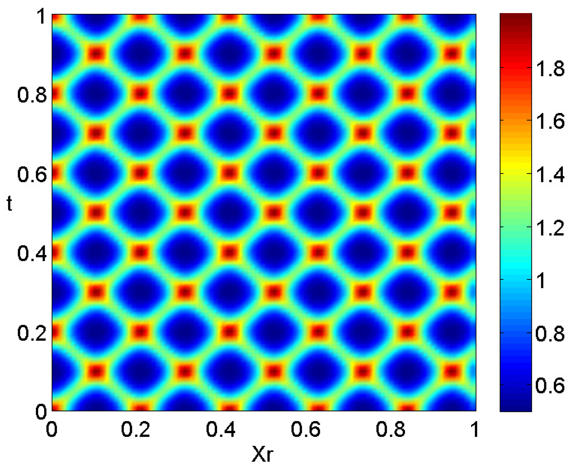
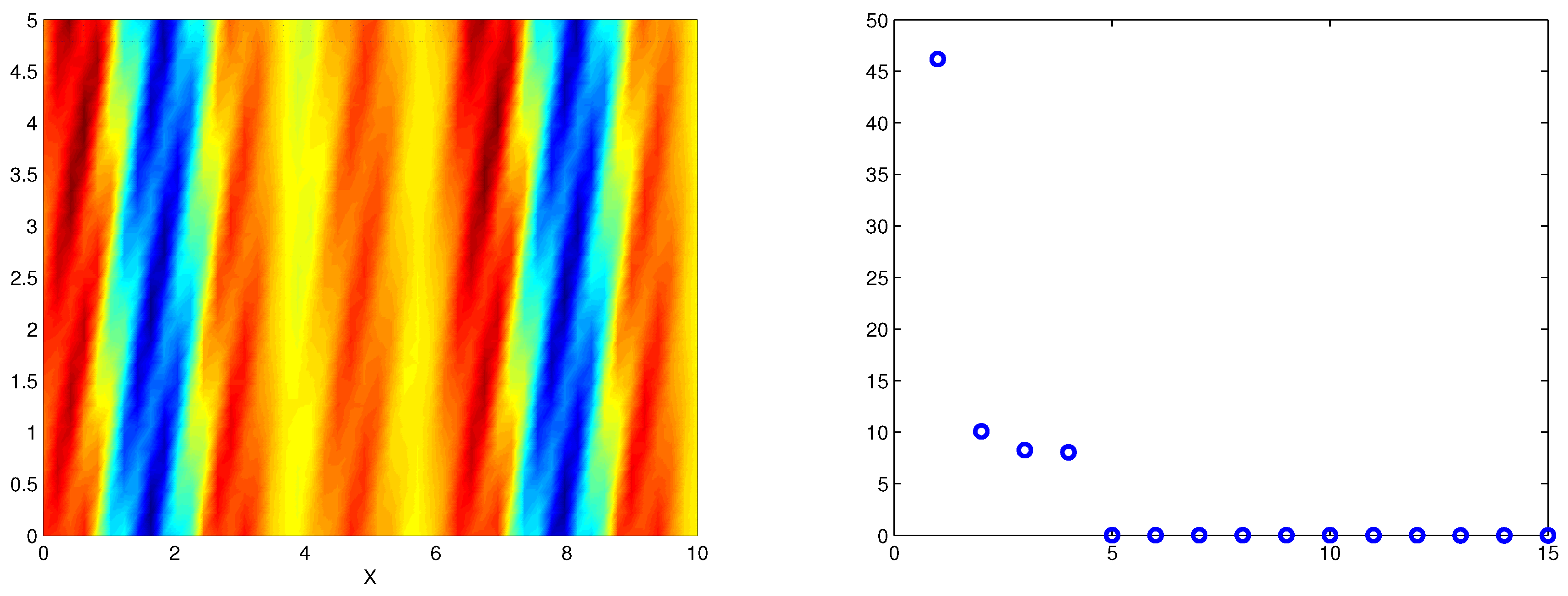
. The colormap of this pattern is depicted in Figure 1(left). This pattern is obtained with spectral spatial and temporal complexities 12 and 4, respectively. This is because it involves 12 wavenumbers:

\pm k_{1}, \pm k_{2}, \pm (k_{1} \pm 1)

and

\pm (k_{2} \pm 1)

, and 4 frequencies:

\pm ω_{1}

and

\pm ω_{2}

. This pattern is spatially periodic, with a period equal to

2 π

, but temporally quasi-periodic.

In order to apply the delay embedding STDMD method, we discretize s and t in the sampled intervals

0 \leq s \leq 10

and

0 \leq t \leq 5

, using 50 and 25 points, respectively. Generated data is

50 \times 25

, but its rank is 4 (see Figure 1(right)), which yields unsatisfactory results with pure temporal DMD method.

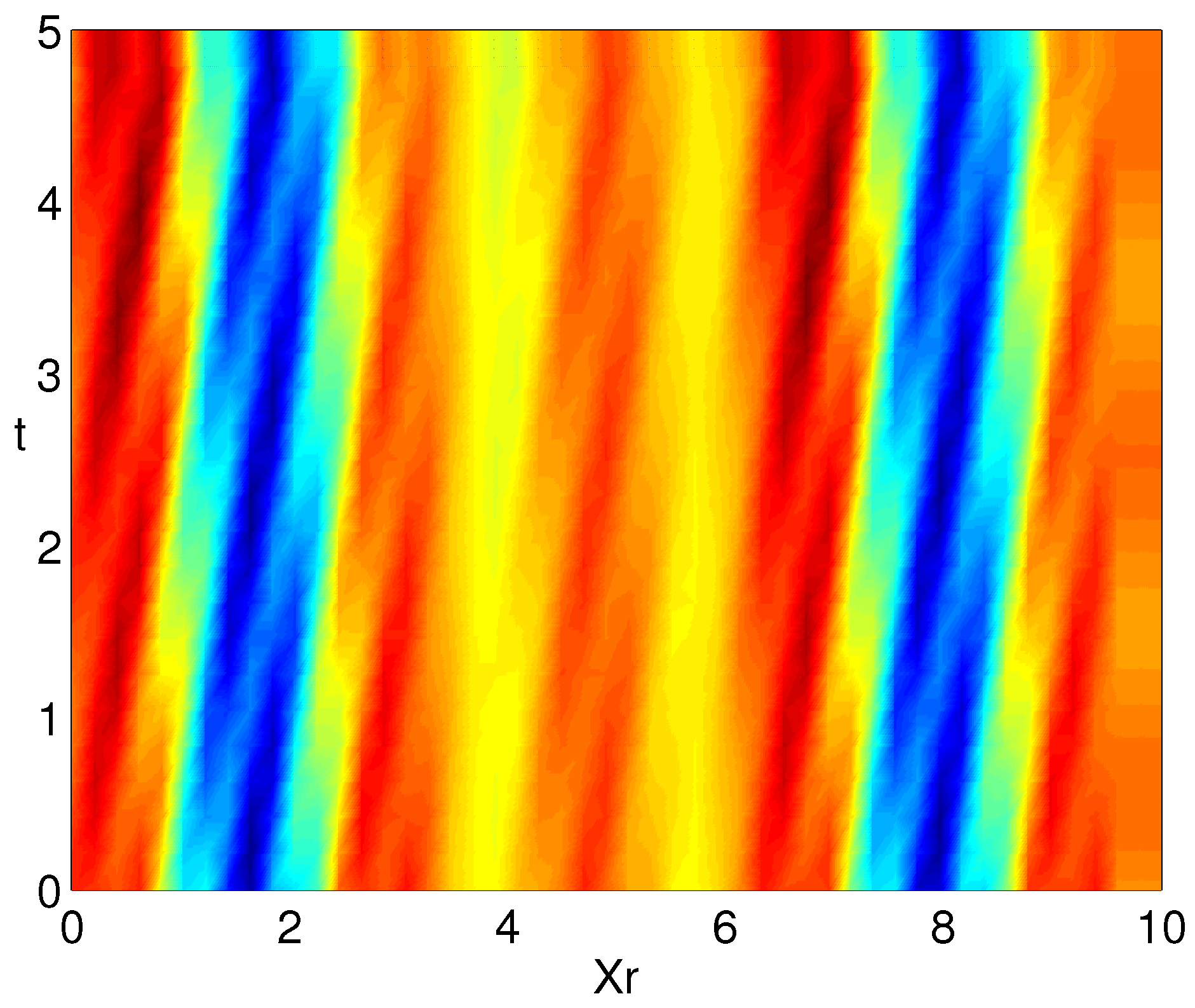
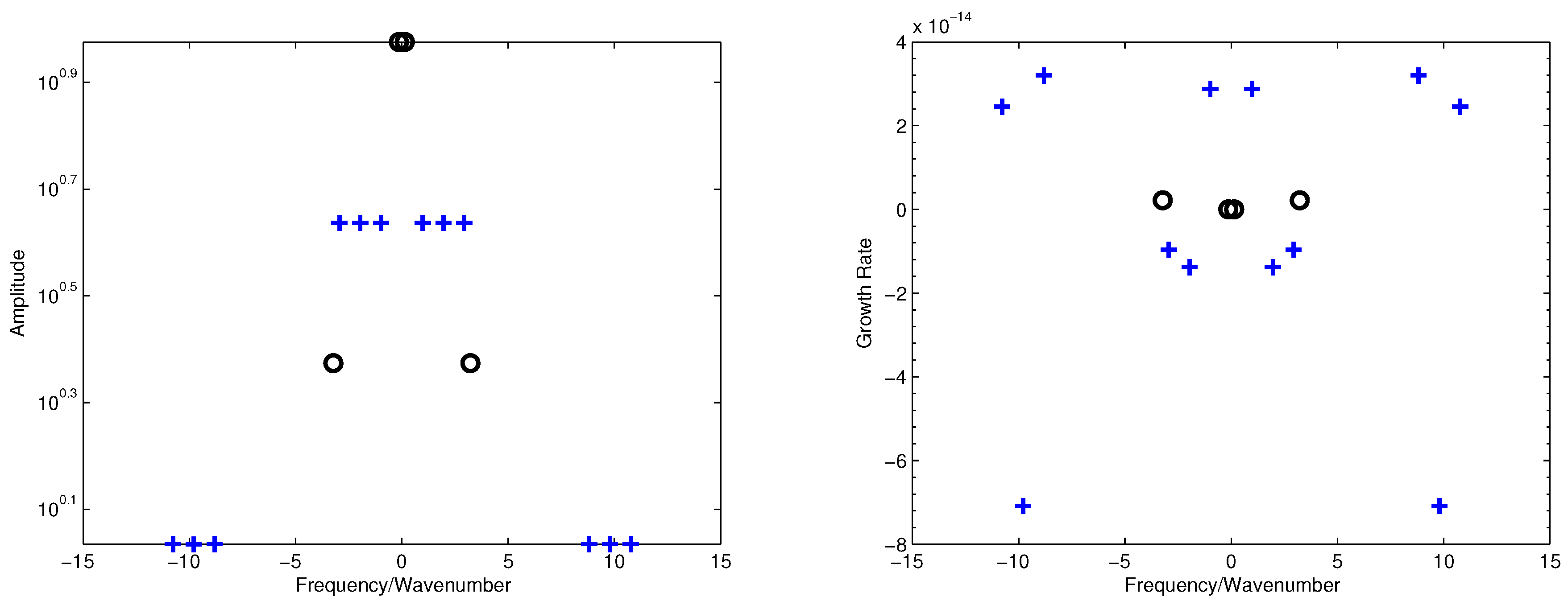
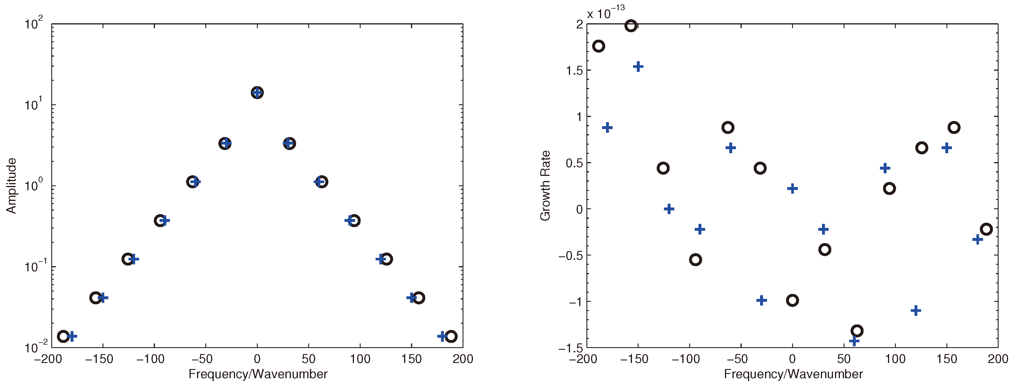
Performing delay embedding STDMD (Algorithm 1), with time delaying index 2 and spatial delaying index 3, we identify the correct 12 wavenumbers and 4 frequencies. See the dinamic reconstruction with delayed STDMD (Algorithm 1) in Figure 2. Figure 3 depicts the amplitudes-frequency and growth rate-frequency diagrams. The results are identical to those in [49], where the STKD method is applied for the same example and input data.

Example 2.

Dynamics of two counter-propagating waves

In this example we consider a dinamics of two counter-propagating waves

x (s, t) = v (s, t) + v (- s, t),

(53)

where v is defined as

v (s, t) = \frac{1}{2} \sum_{- 6}^{6} 3^{- | m |} e^{i m (10 π s + 30 t)} .

(54)

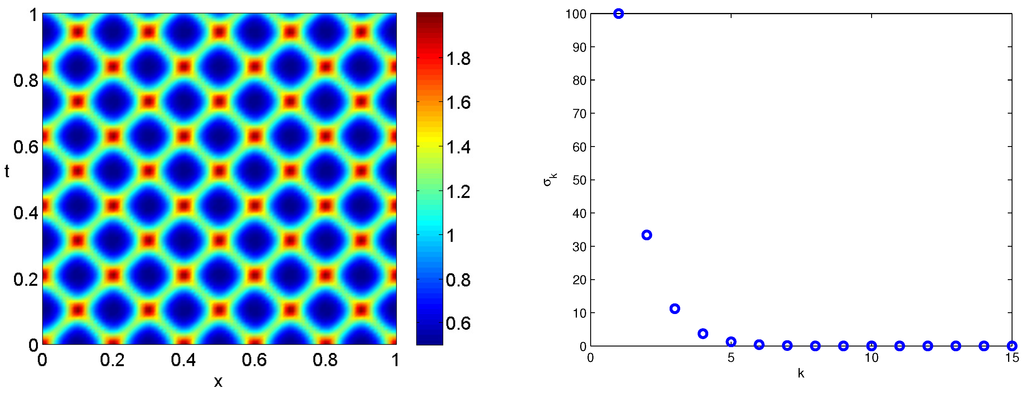
The colormap of this pattern is depicted in Figure 4. The two counter-propagating waves are visible on the chart, but it is seen that the pattern can also be considered as a modulated standing waves, in which the positions of the nodes and crests do not remain constant, but oscillate left and right. The generated data has low-rank structure, which can be seen form the singular values depiction in Figure 4.

If we apply standard DMD approach, then we get only 7 modes and it gives a poor reconstruction of the input data. Instead, if we use delay embedding STDMD (Algorithm 1), with time delaying of 2 and spatial delaying also 2, then we get 13 modes and we reconstruct the input data with greater accuracy. See the dinamic reconstruction with delayed STDMD (Algorithm 1) in Figure 5.

Note that, if we use optimal amplitudes computation, in Algorithm 1, as shown in (33)-(35), then we get better approximation of the dynamics data and and reconstruct the snapshots with a relative RMS error

\sim 1.4 \times 10^{- 12}

. Figure 6 depicts the amplitudes-frequency and growth rate-frequency diagrams.

Note that the counterpart of Eq. (54) is given by

v (s, t) = \frac{1}{2} \sum_{- 6}^{6} 3^{- | m |} e^{30 i m t} cos (10 m π s),

(55)

which implies (from the equality

cos (10 m π s) = cos (- 10 m π s)

) that the spatial complexity is 7, while the spectral complexity is 13. It also follows from (55) that the pattern can be seen as a modulated standing waves.

5. Conclusion

In this paper, we have provided a detailed exposition of two variants for spatio-temporal Dynamic Mode Decomposition (STDMD), namely the parallel methods STDMD and sequential STDMD. We have introduced the matrix representations underlying these techniques, highlighting their respective computational frameworks in analyzing spatio-temporal data. To address some shortcomings of the presented algorithms, which are inherited from the classic DMD algorithm, we have introduced extensions of these approaches incorporating delay embedding techniques. Furthermore, we have conducted numerical experiments to validate the efficacy of the proposed extensions in overcoming the identified limitations of traditional DMD methods. Through these experiments, we have illustrated the enhanced performance of delay embedding STDMD, showcasing its utility in analyzing complex spatio-temporal datasets.

In conclusion, our research contributes to the advancement of spatio-temporal DMD methodologies by introducing extensions that enhance the robustness and accuracy of analysis. Proposed approaches offer valuable tools for researchers and practitioners in diverse fields, enabling deeper insights into the dynamics of complex spatio-temporal systems. We anticipate that our findings will stimulate further research and development in this area, leading to continued advancements in the analysis and understanding of spatio-temporal phenomena.

References

B. Koopman, Hamiltonian systems and transformations in Hilbert space, Proceedings of the National Academy of Sciences, (1931), 17: pp. 315–318.
I. Mezić. Spectral properties of dynamical systems, model reduction and decompositions. Nonlin. Dynam., 41(1-3):309-325, August 2005.
P. J. Schmid and J. Sesterhenn. Dynamic mode decomposition of numerical and experimental data. In 61st Annual Meeting of the APS Division of Fluid Dynamics. American Physical Society, November 2008.
C. W. Rowley, I. Mezić, S. Bagheri, P. Schlatter, and D. S. Henningson. Spectral analysis of nonlinear flows. J. Fluid Mech., 641:115-127, December 2009.
P. J. Schmid. Application of the dynamic mode decomposition to experimental data. Exp. Fluids, 50(4):1123-1130, April 2011.
J. L. Proctor and P. A. Eckhoff, Discovering dynamic patterns from infectious disease data using dynamic mode decomposition, International health, 7 (2015), pp. 139-145.
J. Grosek, J. Nathan Kutz, Dynamic Mode Decomposition for Real-Time Background/Foreground Separation in Video, arXiv: 1404.7592.
B. W. Brunton, L. A. Johnson, J. G. Ojemann, and J. N. Kutz, Extracting spatial-temporal coherent patterns in large-scale neural recordings using dynamic mode decomposition, Journal of Neuroscience Methods, 258 (2016), pp. 1-15.
J. Mann and J. N. Kutz, Dynamic mode decomposition for financial trading strategies, Quantitative Finance, (2016), pp. 1-13.
Ling-xiao Cui, Wen Long, 2016. "Trading strategy based on dynamic mode decomposition: Tested in Chinese stock market," Physica A: Statistical Mechanics and its Applications, Elsevier, vol. 461(C), pages 498-508.
D. P. Kuttichira, E. A. Gopalakrishnan, V. K. Menon and K. P. Soman, "Stock price prediction using dynamic mode decomposition," 2017 International Conference on Advances in Computing, Communications and Informatics (ICACCI), Udupi, India, 2017, pp. 55-60. [CrossRef]
E. Berger, M. Sastuba, D. Vogt, B. Jung, and H. B. Amor, Estimation of perturbations in robotic behavior using dynamic mode decomposition, Journal of Advanced Robotics, 29 (2015), pp. 331-343.
P. J. Schmid. Dynamic mode decomposition of numerical and experimental data. J. Fluid Mech., 656:5-28, August 2010.
Seena and H. J. Sung. Dynamic mode decomposition of turbulent cavity ows for selfsustained oscillations. Int. J. Heat Fluid Fl., 32(6):1098-1110, December 2011.
I. Mezić. Analysis of fluid flows via spectral properties of the Koopman operator. Annu. Rev. Fluid Mech., 45:357-378, 2013.
J. H. Tu, C. W. Rowley, D. M. Luchtenburg, S. L. Brunton, J. N. Kutz. On dynamic mode decomposition: Theory and applications. Journal of Computational Dynamics, 1 (2) : 391-421, 2014.
J. Nathan Kutz, Steven L. Brunton, Bingni W. Brunton, and Joshua Proctor (2016). Dynamic Mode Decomposition: Data-Driven Modeling of Complex Systems, SIAM 2016, ISBN 978-1-611-97449-2, pp. 1-234.
Zhe Bai, Eurika Kaiser, Joshua L. Proctor, J. Nathan Kutz, Steven L. Brunton, Dynamic Mode Decomposition for CompressiveSystem Identification, AIAA Journal, Vol. 58, No. 2, 20, pp. 561-574.
S.L. Brunton, M.Budišić, E.Kaiser, and J.N. Kutz, Modern Koopman Theory for Dynamical Systems, SIAM Review 2022 64:2, 229-340. [CrossRef]
K. K. Chen, J. H. Tu, and C. W. Rowley. Variants of dynamic mode decomposition: Boundary condition, Koopman, and Fourier analyses. J. Nonlinear Sci., 22:887-915, 2012. [CrossRef]
Williams, M. O., Hemati, M. S., Dawson, S. T. M., Kevrekidis, I. G., and Rowley, C. W. (2016). Extending Data-Driven Koopman Analysis to Actuated Systems. IFAC-PapersOnLine, 49(18), 704-709. [CrossRef]
S. Le Clainche, J.M.Vega, J. Soria, Higher order dynamic mode decomposition of noisy experimental data: The flow structure of a zero-net-mass-flux jet, , Experimental Thermal and Fluid Science, vol. 88, 2017. [CrossRef]
S. Anantharamu, K. Mahesh, A parallel and streaming Dynamic Mode Decomposition algorithm with finite precision error analysis for large data, Journal of Computational Physics, Volume 380, 2019. [CrossRef]
T. Sayadi, P.J. Schmid, Parallel data-driven decomposition algorithm for large-scale datasets: with application to transitional boundary layers. Theor. Comput. Fluid Dyn. 30, 415-426 (2016). [CrossRef]
K.R. Maryada, S.E. Norris, Reduced-communication parallel dynamic mode decomposition, Journal of Computational Science, Volume 61, 2022. [CrossRef]
B. Li, J. Garicano-Menaab, E. Valero, A dynamic mode decomposition technique for the analysis of nonuniformly sampled flow data, Journal of Computational Physics, Volume 468, 2022. [CrossRef]
E. Smith, I. Variansyah, R. McClarren, Variable Dynamic Mode Decomposition for Estimating Time Eigenvalues in Nuclear Systems, https://arxiv.org/abs/2208.10942v1.
M.R. Jovanovic, P.J. Schmid, J.W. Nichols, Sparsity-promoting dynamic mode decomposition, Physics of Fluids 26, 2014. [CrossRef]
F. Guéniat, L. Mathelin, L.R. Pastur, A dynamic mode decomposition approach for large and arbitrarily sampled systems, Phys Fluids 27, 2014. [CrossRef]
N. Cassamo, J.W. van Wingerden, On the Potential of Reduced Order Models for Wind Farm Control: A Koopman Dynamic Mode Decomposition Approach. Energies 2020, 13, 6513. [CrossRef]
T.T. Ngo, V.Nguyen, X.Q. Pham, M.A.Hossain, E.N. Huh, Motion Saliency Detection for Surveillance Systems Using Streaming Dynamic Mode Decomposition. Symmetry 2020, 12, 1397. [CrossRef]
O.P. Babalola, V. Balyan, WiFi Fingerprinting Indoor Localization Based on Dynamic Mode Decomposition Feature Selection with Hidden Markov Model. Sensors 2021, 21, 6778. [CrossRef]
M. Lopez-Martin, A. Sanchez-Esguevillas, L. Hernandez-Callejo, J.I. Arribas, B. Carro, Novel Data-Driven Models Applied to Short-Term Electric Load Forecasting. Appl. Sci. 2021, 11, 5708. [CrossRef]
S. Surasinghe, E.M. Bollt, Randomized Projection Learning Method for Dynamic Mode Decomposition. Mathematics 2021, 9, 2803. [CrossRef]
C.Y. Li, Z. Chen, T.K.T. Tse, A parametric and feasibility study for data sampling of the dynamic mode decomposition: range, resolution, and universal convergence states. Nonlinear Dyn 107, 3683-3707 (2022). [CrossRef]
I. Mezić, On Numerical Approximations of the Koopman Operator. Mathematics 2022, 10, 1180. [CrossRef]
G. Nedzhibov, Dynamic Mode Decomposition: a new approach for computing the DMD modes and eigenvalues, Ann. Acad. Rom. Sci. Ser. Math. Appl. Vol. 14, No. 1-2/2022. [CrossRef]
Nedzhibov, G. On Alternative Algorithms for Computing Dynamic Mode Decomposition. Computation 2022, 10, 210. [CrossRef]
Nedzhibov, G. An Improved Approach for Implementing Dynamic Mode Decomposition with Control. Computation 2023, 11, 201. [CrossRef]
G. Nedzhibov, Online Dynamic Mode Decomposition: an alternative approach for low rank datasets, Annals of the Academy of Romanian Scientists: Series on Mathematics and its ApplicationsThis link is disabled., 2023, 15(1-2), pp. 229–249. [CrossRef]
Nedzhibov, G. Extended Online DMD and Weighted Modifications for Streaming Data Analysis. Computation 2023, 11, 114. [CrossRef]
H. Arbabi and I. Mezić, Ergodic Theory, Dynamic Mode Decomposition, and Computation of Spectral Properties of the Koopman Operator, SIAM Journal on Applied Dynamical Systems, 16 (2017), pp. 2096–2126. [CrossRef]
M. Kamb, E. Kaiser, S. L. Brunton, and J. N. Kutz, Time-delay observables for Koopman: Theory and applications, SIAM J. Appl. Dyn. Syst., 19 (2020), pp. 886–917. [CrossRef]
J.N. Juang and R. S. Pappa, An eigensystem realization algorithm for modal parameter identification and model reduction, J. Guidance Control Dyn., 8 (1985), pp. 620–627.
R. Vautard and M. Ghil, Singular spectrum analysis in nonlinear dynamics, with applications to paleoclimatic time series, Phys. D, 35 (1989), pp. 395–424.
S. L. Brunton, B. W. Brunton, J. L. Proctor, E. Kaiser, and J. N. Kutz, Chaos as an intermittently forced linear system, Nature Commun., 8 (2017), 19.
F. Takens, Detecting strange attractors in turbulence, in Dynamical Systems and Turbulence, Lecture Notes in Math. 898, Springer, Berlin, 1981.
A.S. Sharma, I. Mezić, B.J. McKeon, Correspondence between Koopman mode decomposition, resolvent mode decomposition, and invariant solutions of the Navier-Stokes equations, Phys. Rev. Fluids 1 (2016) 032402.
Clainche, S.L., Vega, J.M. Spatio-Temporal Koopman Decomposition. J Nonlinear Sci 28, 1793-1842 (2018). [CrossRef]
J.M. Vega, S. Le Clainche, Higher Order Dynamic Mode Decomposition and Its Applications, Elsevier, 2020.
S. Le Clainche, J.M. Pérez, J.M. Vega, Spatio-temporal flow structures in the three-dimensional wake of a circular cylinder, Fluid Dyn. Res. 50 (2018) 051406.
W. Lu, G. Huang, J. Wang, S. Hong, Spatio-temporal dynamic mode decomposition in a shear layer flow, Aerosp. Sci. Technol. 91 (2019) 263-271.
D. Giannakis, J. D. Giannakis, J. Slawinska, Z. Zhao, Spatiotemporal Feature Extraction with Data-Driven Koopman Operators, JMLR: Workshop and Conference Proceedings 44 (2015) 103-115.
K. Kikuchi and B. Wang. Spatiotemporal wavelet transform and the multiscale behavior of the Madden-Julian oscillation. J. Climate, 23:3814–3834, 2010. [CrossRef]

Figure 1. Spatio-temporal color map for the dynamics defined by (53),(left panel), and first 15 singular values of the generated data (right panel).

Figure 2. Spatio-temporal color map of reconstructed data computed by delay embedding STDMD (Algorithm 1).

Figure 3. Left panel: Spatial amplitudes-wavenumber (’+’) and temporal amplitudes-frequency (’o’); Right panel: Spatial growth rate-wavenumber (’+’) and temporal growth rate-frequency (’o’).

Figure 4. Spatio-temporal color map for the dynamics defined by (53),(left panel), and first 15 singular values of the generated data (right panel).

Figure 5. Spatio-temporal color map of reconstructed data computed by delay embedding STDMD (Algorithm 1).

Figure 6. Left panel: Spatial amplitudes-wavenumber (’+’) and temporal amplitudes-frequency (’o’); Right panel: Spatial growth rate-wavenumber (’+’) and temporal growth rate-frequency (’o’).

Disclaimer/Publisher’s Note: The statements, opinions and data contained in all publications are solely those of the individual author(s) and contributor(s) and not of MDPI and/or the editor(s). MDPI and/or the editor(s) disclaim responsibility for any injury to people or property resulting from any ideas, methods, instructions or products referred to in the content.

© 2024 by the authors. Licensee MDPI, Basel, Switzerland. This article is an open access article distributed under the terms and conditions of the Creative Commons Attribution (CC BY) license (http://creativecommons.org/licenses/by/4.0/).

Copyright: This open access article is published under a Creative Commons CC BY 4.0 license, which permit the free download, distribution, and reuse, provided that the author and preprint are cited in any reuse.

MDPI Initiatives

Important Links

Choose an area of interest and we will send you notifications of new preprints at your preferred frequency.

Disclaimer

Delay Embedding Spatio-Temporal Dynamic Mode Decomposition

Abstract

1. Introduction

1.1. Dynamic mode decomposition

1.2. Reduced-order DMD operator

1.3. Optimal amplitudes of DMD modes

1.4. Delay embedding Dynamic Mode Decomposition

2. Spatio-Temporal DMD

2.1. Parallel STDMD

2.2. Sequential STDMD

3. Delay embedding STDMD

4. Numerical examples

5. Conclusion

References

MDPI Initiatives

Important Links

Subscribe