Submitted:
18 February 2024
Posted:
19 February 2024
You are already at the latest version
Abstract
Keywords:
1. Introduction
2. Related Works
3. Background
3.1. Artificial Immune Recognition system v2.0
3.2. Recurrent Neural Netwrk (RNN)

3.3. Adaboost classification techniques

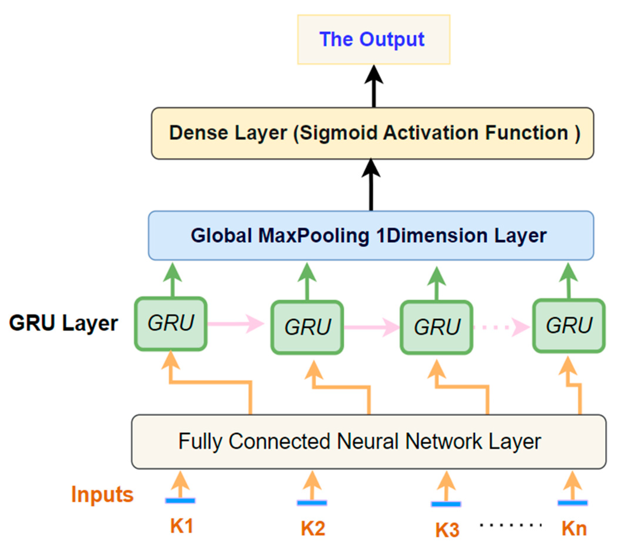
3. The Architecture of the Proposed Deep Learning Model for the Prediction of Students' Performance in Educational Institutions
3.1. Maxpooling:
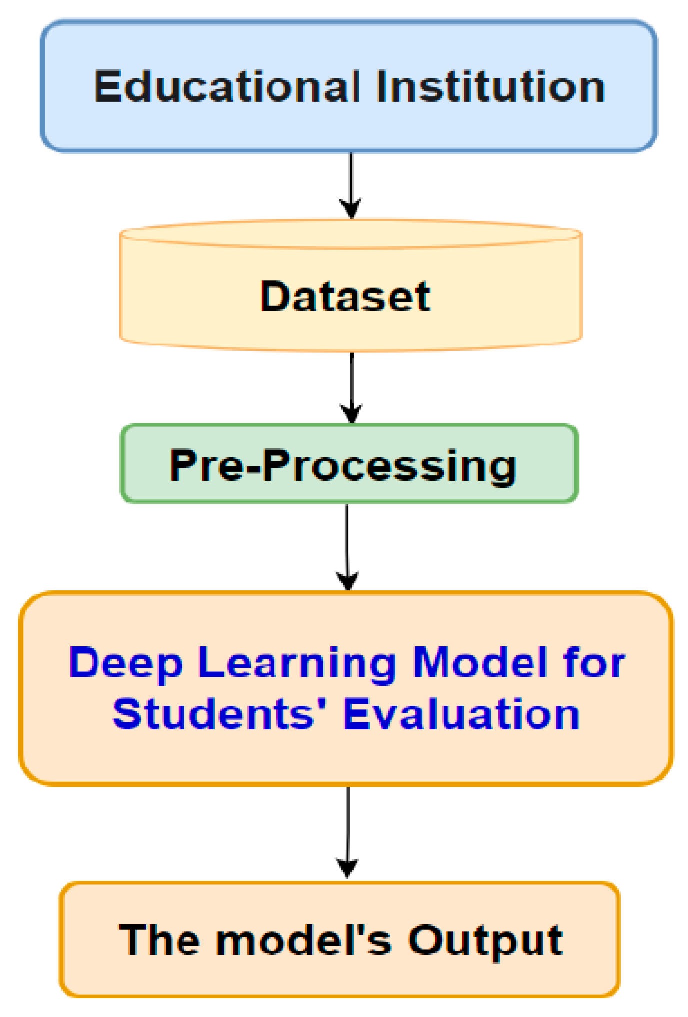
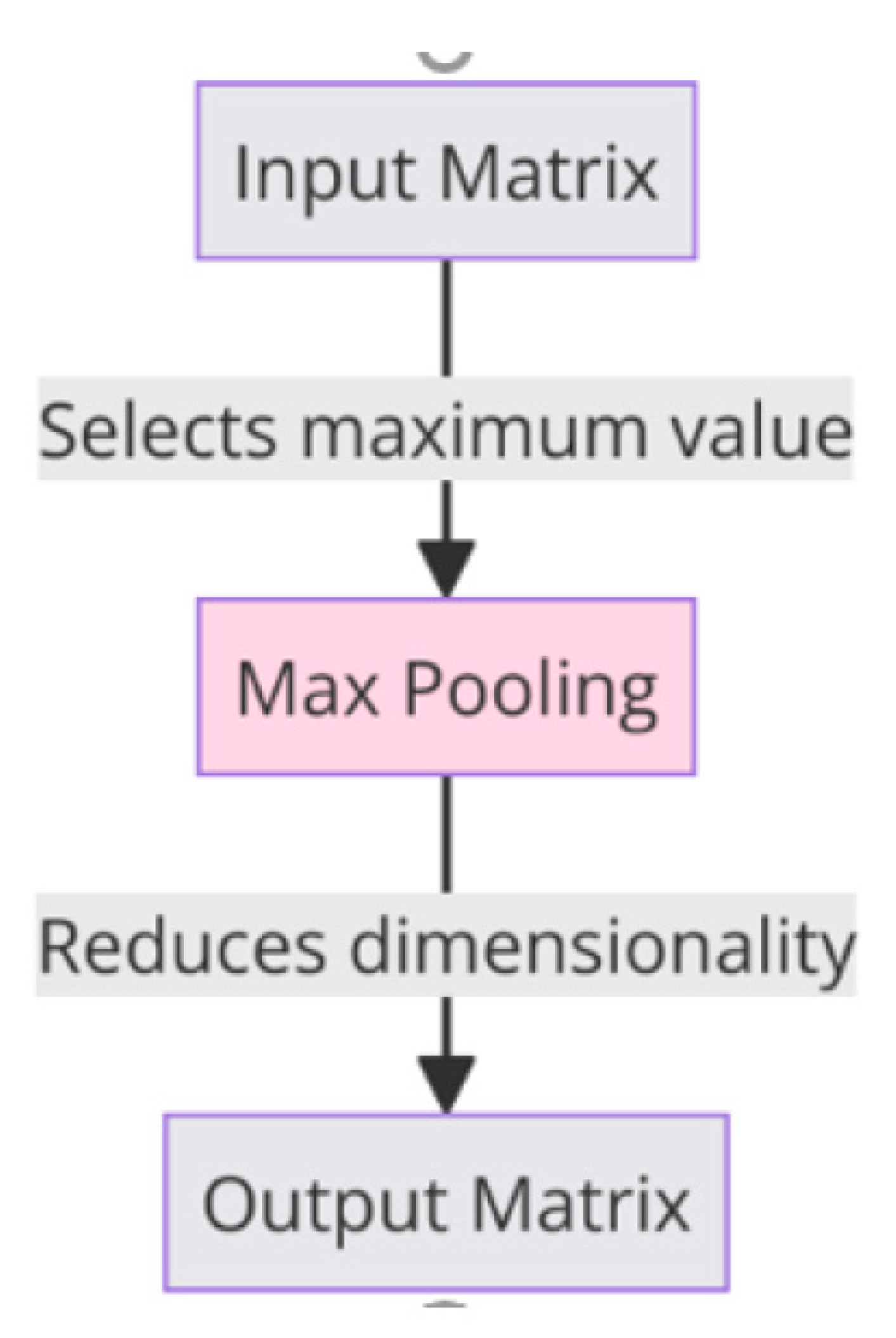
3. Experiments
3.1. Datasets
| Feature | Explanation | Values |
|---|---|---|
| Exam | The Three Year Degree Six semester Examinations | {'BA', ‘BSC’ } Two tests are occupied into account, i.e. BA and BSc |
| IN_Sem1 | Major/Honours Topics Of Bachelor and Master Programs |
{'ENGM','PHYM', etc.} ENGM- Major/Honours in English PHYM- Major/Honours in Physics |
| IN_Sem2 | Internal evaluation Grades acquired in the BA/BSc 1st Semester Examination |
Maximum marks 20 Marks achieved by the students in the range 1 to 20. Mean: 15.66257 Standard Deviation SD: 2.593816 |
| IN_Sem3 | Internal evaluation Grades obtained in the BA/BSc 3rd Semester Examination |
Maximum marks 40 Marks achieved by the students in the range 1 to 40. Mean: 31.95765 Standard Deviation SD: 5.101312 |
| IN_Sem4 | Internal evaluation Grades obtained in the BA/BSc 4th Semester Examination |
Maximum marks 40 Marks achieved by the students in the range 1 to 40. Mean: 30.80859 Standard Deviation: 5.43647 |
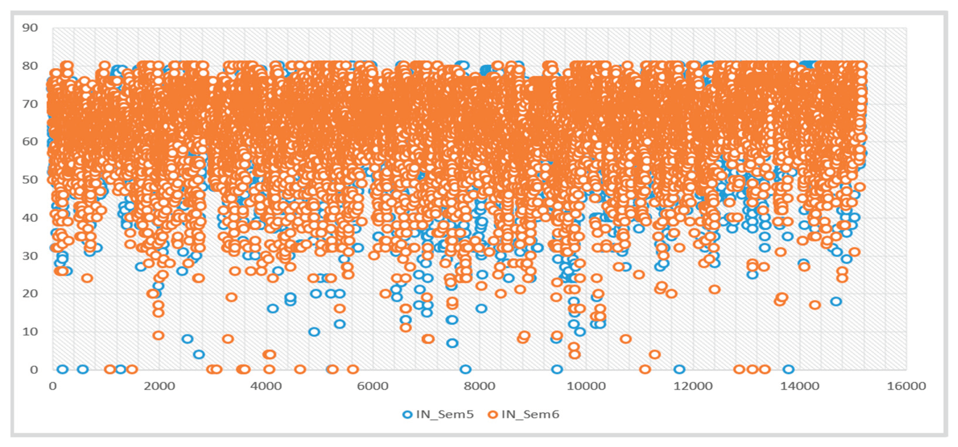
| IN_Sem5 | Internal evaluation Grades obtained in the BA/BSc 5th Semester Examination |
Maximum marks 80 Marks achieved by the students in the range 1 to 80. Mean: 64.71536 Standard Deviation: 10.18944 |
| IN_Sem6 | Internal evaluation Grades obtained in the BA/BSc 6th Semester Examination |
Maximum marks 80 Marks achieved by the students in the range 1 to 80. Mean: 64.79921 Standard Deviation: 10.3252 |
| InPc | The overall percentage secured by the candidate in all the six semesters in the internalassessments |
Mean: 80.44676 Standard Deviation: 11.01706 |
| Result | The overall result of the applicant established the all the six semesters theory and interior assessment |
{‘Pass’, ‘Fail’} If a student secures 40% or overhead, he is termed as ‘Pass’ Else ‘Fail’ |
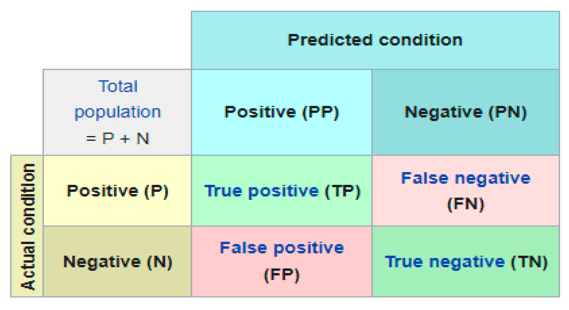
3.2. Evaluation Metrics
3.2. Results and the Proposed Model Hyperparameters
| Layer (Type) | Output Shape | Parameters No. |
|---|---|---|
| Input_1 (inputLayer) | (None, 10, 1) | 0 |
| Word_dense (Dense) | (None, 10, 100) | 200 |
| Gru (GRU) | (None, 10, 256) | 274944 |
| Global_max_pooling (Global MaxpoolingID | (None, 256) | 0 |
| Dense | (None, 2) | 514 |
| Total Parameters: 275,658 | ||
| Trainable Parameters: 275,658 | ||
| Non-Trainable Parameters: 275,658 | ||
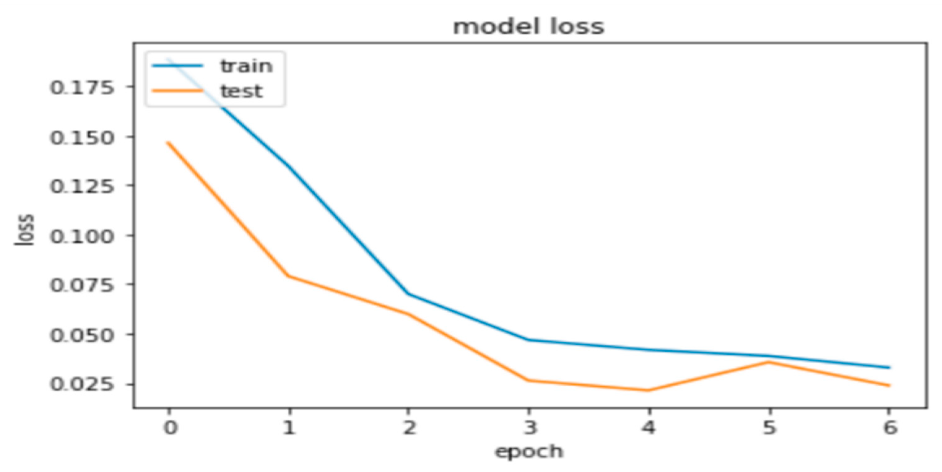
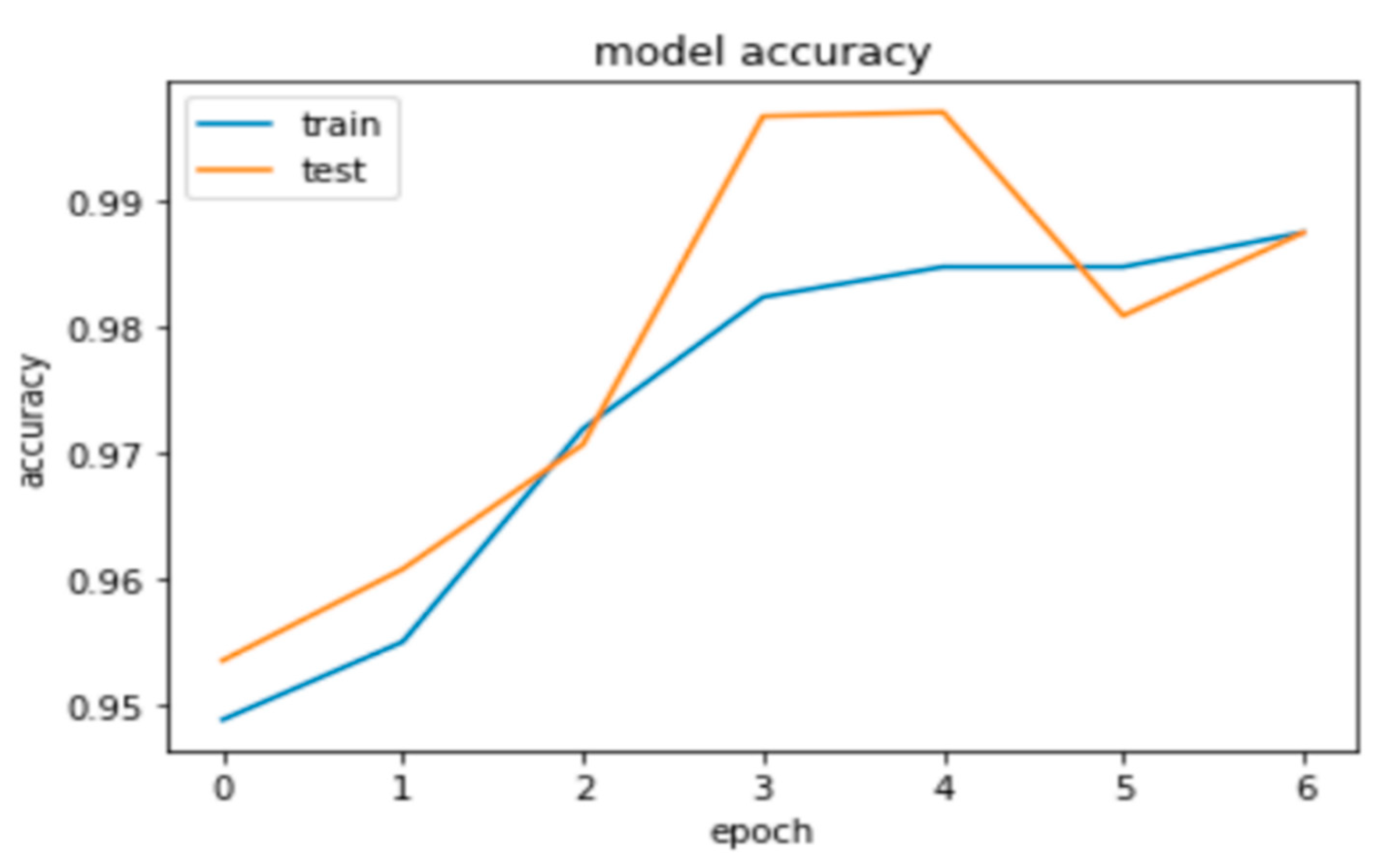
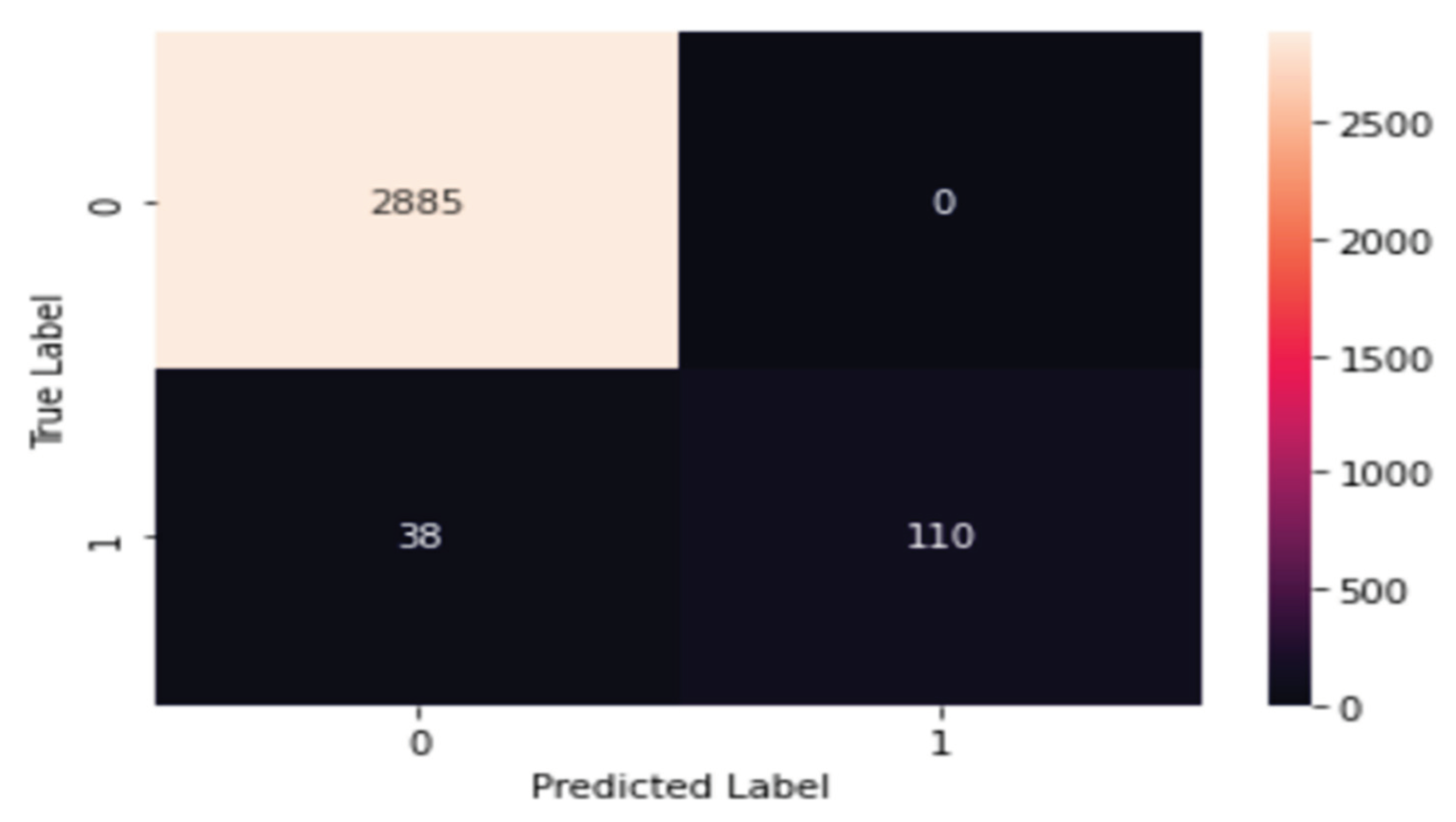
| The Classifier | Precision | Recall | F-Score | Accuracy |
|---|---|---|---|---|
| RNN Model | 0.96 | 0.99 | 0.98 | 95.34 |
| ARD V.2 | 0.926 | 0.932 | 0.939 | 93.18 |
| AdaBoost | 0.934 | 0.946 | 0.939 | 94.57 |
| The Proposed model | 0.986 | 0.963 | 0.974 | 99.70 |
5. Conclusion
Author Contributions
Funding
Data Availability Statement
Conflicts of Interest
References
- Agrawal, R.S; Pandya, M.H. Survey of papers for Data Mining with Neural Networksto Predict the Student's Academic Achievements. Intern Journal of Comp Scie Trends and Techn (IJCST) 2015, 3, 15. [Google Scholar]
- Beikzadeh, M. R.; Delavari. N. A New Analysis Model for Data Mining Processes in Higher Educational Systems. In Proceedings of the 6th Information Technology Based Higher Education and Training, 7-9 July 2005.
- Steiner, C.; Kickmeier-Rust, M.; Albert, D. Learning Analytics and Educational Data Mining: An Overview of Recent Techniques. Learning analytics for and in serious games 2014, 6–15. [Google Scholar]
- Khan, S.; Alqahtani, S. Big Data Application and its Impact on Education. Inter Journ of Emer Techno in Learning (iJET0) 2020, 15, 36–46. [Google Scholar] [CrossRef]
- Ouatik, F.; Erritali, M.; Ouatik, F.; Jourhmane, M. Predicting Student Success Using Big Data and Machine Learning Algorithms. Intern Journal of Eme Technol in Learn (iJET) 2022, 17. [Google Scholar] [CrossRef]
- Philip Chen, C.L.; Zhang, C.-Y. Data-intensive applications, challenges, techniques, and technologies: A survey on Big Data Inform. Sci 2014. [CrossRef]
- H, Shuliang.; Cuibi, Y. Learners' Autonomous Learning Behavior in Distance Reading Based on Big Data. Intern Jour of Emer Techn in Learning (iJET) 2022. [CrossRef]
- ALSHARAIAH, M A.; BANIATA, L.H.; ALADWAN, O.; AbuaAlghanam, O.; Abushareha, A.A.; Abuaalhaj, M.; Sharayah, Q.; Baniata, M. SOFT VOTING MACHINE LEARNING CLASSIFICATION MODEL TO PREDICT AND EXPOSE LIVER DISORDER FOR HUMAN PATIENTS. Journal of Theor and Applied Information Technology 2022, ,100, 4554 – 4564.
- Alsharaiah, M A.; Baniata, L.H.; Adwan, O; Abu-Shareha, A. A ; Abuaalhaj, M.; Kharma, Q.; Hussein, A.; Abualghanam, O.; Alassaf, N.; Baniata, M. Attention-based Long Short Term Memory Model for DNA Damage Prediction in Mammalian Cells. International Journal of Advanced Computer Science and Applications 2022, 13, 91–99.
- Alsharaiah, M.A.; Baniata, L.H.; Al Adwan, O.; Abuaalghanam, O.; Abu-Shareha, A.A; Alzboon, L.; Mustafa, N; Baniata, M. Neural Network Prediction Model to Explore Complex Nonlinear Behavior in Dynamic Biological Network. Neural Network Prediction Model to Explore Complex Nonlinear Behavior in Dynamic Biological Network. International Journal of Interactive Mobile Technologies 2022, 16, 32–51.
- Krish, K.Data-Driven Architecture for Big Data. Data Warehousing in the Age of BigData.," MK of BigData.-MK Series on Business Intelligence,2013.
- Kastranis, A. Artificial Intelligence for People and Business," O’ Reily Media Inc.: Sebastopol, CA, USA, 2019.
- Siemens, G.; Baker, R.S. Learning analytics and educational data mining: towards communication and collaboration. 2012. [CrossRef]
- Aher, S.B. Data Mining in Educational System using WEKA, 2011.
- Sunita, B.; Aher.; Lobo, L.; M, R.J. Mining Association Rule in Classified Data for Course Recommender System in E-Learning. International Journal of Computer Applications 39, 1–7. [CrossRef]
- Felix, I.M.; Ambrosio, A.P.; Neves, P.S.; Siqueira, J.; Brancher, J.D. Moodle Predicta: A Data Mining Tool for Student Follow Up. CSEDU 2017. [CrossRef]
- International Educational Data Mining Society, [Online]. Available: www.educationaldatamining.org.
- Gijbels, D.; Van de Watering, G.; Dochy, F.; Van den Bossche, P. The relationship between students' approaches to learning and the assessment of learning outcomes. European Journal of Psychology of Education, 20, 327-341. [CrossRef]
- Elhaj, M.A.E.; Bashir, S.G; Abdullahi, I.; Onyema, E.M.; Hauw. Evaluation of the Performance of K-Nearest Neighbor Algorithm in Determining Student Learning Style. Evaluation of the Performance of K-Nearest Neighbor Algorithm in Determining Student Learning Style. Intern Jour of Innov Sci, Engine. & Techogy 2020, 7, 2348–7968.
- Anjali J.; A REVIEW OF MACHINE LEARNING IN EDUCATION," Journal of Emerging Technologies and Innovative Research (JETIR), 6 ,2019.
- Hussain, S.; Dahan N. A., Ba-Alwib F. M., Najoua R. Educational Data Mining and Analysis of Students' Academic Performance Using WEKA. Indonesian Journal of Electrical Engineering and Computer Science 2018, 9. [CrossRef]
- López, M. Classification via clustering for predicting final marks based on student participation in forums, In the Proceedings of the 5th International Conference on Educational Data Mining, 2012.
- Klašnja-Milićević, A. E-Learning personalization based on hybrid recommen recommendation strategy and learning style identification. Computers & Education, 56, 2011. [CrossRef]
- Ayesha, S. Data Mining Model for Higher Education System.European Journal of Scientific Research. 43, 1, 24 – 29, 2010.
- Permata Alfiani, A.; Ayu Wulandari, F. Mapping Student's Performance Based on the Data Mining Approach (A Case Study)," Agriculture and Agricultural Science Procedia 2015, 173–177, 2015. [CrossRef]
- Bovo, A. Clustering moodles data as a tool for profiling students. In the proceedings of International Conference on E-Learning and E-Technologies in Education (ICEEE) 2013, 121-126. [CrossRef]
- Antonenko, P.D.; Toy, S.; Niederhauser, D.S. Using cluster analysis for data mining in educational technology research. Educational Technology Research and Development 2012, 60, 383–398. [Google Scholar] [CrossRef]
- Bendangnuksung , Prabu P. Students' Performance Prediction Using Deep Neural Network. International Journal of Applied Engineering Research, 13, 2018.
- Dey, R.; Salem, F.M. Gate-Variants of Gated Recurrent Unit (GRU) Neural Networks, 2017.
- Cho, Kyunghyun; van Merrienboer, Bart; Bahdanau, DZmitry; Bengio, Yoshua. On the Properties of Neural Machine Translation: Encoder-Decoder Approaches, 2014.
- Ravanelli, M; Brakel, P; Omologo, M; Bengio, Y. Light Gated Recurrent Units for Speech Recognition. IEEE Transactions on Emerging Topics in Computational Intelligence 2018. [CrossRef]
- John Pomerat, Aviv Segev, and Rituparna Datta, On Neural Network Activation Functions and Optimizers in Relation to Polynomial Regression," IEEE International Conference on Big Data (Big Data)., 2019. [CrossRef]
- Zijun Zhang, improved Adam Optimizer for Deep Neural Networks, IEEE, 2018. [CrossRef]
- k. document. [Online]. Available: https://keras.io/search.html?query=maxpooling.
- D. l. :. Keras. [Online]. Available: https://keras.io/api/layers/core_layers/dense/.
- Peng, Y., & Lu, B., "Hybrid learning clonal selection algorithm.," Inf. Sci., pp. 296, 128, 2015. [CrossRef]
- Saidi, M., Chikh, A., Settouti, N . Automatic Identification of Diabetes Diseases using an Artificial Immune Recognition System2 AIRS2) with a Fuzzy K-Nearest Neighbor," CIIA, 2011.
- Abiodun, O. I.; Jantan, A.; Omolara, A. E.; Dada, K.V.; Mohamed, N. A.; Arshad, H. State-of-the-art in artificial neural network applications: A survey. Heliyon 2018. [CrossRef]
- Tealab, A. Time series forecasting using artificial neural networks methodologies: A systematic review. Future Computing and Informatics Journal 2018. [CrossRef]
- Sadiq. H.; Zahraa, F.M.; Yass, K. S. Prediction Model on Student Performance based on Internal Assessment using Deep Learning. S. Prediction Model on Student Performance based on Internal Assessment using Deep Learning. International Journal of Emerging Technologies in Learning 2019, 14. [CrossRef]
- Mukherjee, C.; Rudin.; R. Schapire, The rate of convergence of AdaBoost. Journal of Machine Learning Research 2013,14, 315-2347.
- Tharwat, A. Classification assessment methods. Applied Computing and Informatics 2018. [CrossRef]
- Powers, D.MW. Evaluation: From Precision, Recall and F-Measure to ROC, Informedness, Markedness & Correlation. Journal of Machine Learning Technologies 2011, 2, 37–63. [Google Scholar] [CrossRef]
Disclaimer/Publisher’s Note: The statements, opinions and data contained in all publications are solely those of the individual author(s) and contributor(s) and not of MDPI and/or the editor(s). MDPI and/or the editor(s) disclaim responsibility for any injury to people or property resulting from any ideas, methods, instructions or products referred to in the content. |
© 2024 by the authors. Licensee MDPI, Basel, Switzerland. This article is an open access article distributed under the terms and conditions of the Creative Commons Attribution (CC BY) license (http://creativecommons.org/licenses/by/4.0/).


