There is a common issue regarding data protection and privacy, such as costs or production factors, in enterprises. Of course, data can be computed and encrypted, but if an outsider gains access to encrypted data and the data functions for cost and production, it’s only a matter of time before the adversary reconstructs the real data. There are various published examples of encryption. In the article by [1] from 2017, authors present a general construction of functional encryption with inner product, which is resistant to chosen plaintext attacks (IND-FE-CCA), based on hash functions with homomorphic properties. Authors demonstrate specific implementations based on the assumptions of Decisional Composite Residuosity (DCR), Decisional Diffie-Hellman (DDH), and more generally, Matrix DDH. The article titled "Azure Functions security" [7] published on the Microsoft Learn website describes services and actions related to security that can be applied to Azure serverless functions. The article provides guidelines and resources to help develop secure code and deploy secure applications to the cloud. In the article [2] , the authors present a general scheme and syntax for functional encryption and demonstrate how existing encryption concepts, such as attribute-based encryption and many others, can be elegantly expressed as specific functionalities of functional encryption. Defining the security of abstract functional encryption proves to be very non-trivial. Authors present several definitions and challenges related to functional encryption.

The aim of the Section 2 is to ensure data security as well as the security of cost and production functions.The production function and the cost function are closely related because the cost of producing a certain quantity of a product depends on the inputs of production factors and their prices. The cost function $TC$ shows the minimum cost of producing a given quantity of a product at given input prices. The cost function can be expressed as the sum of fixed costs F and variable costs $CV$, which depend on the production quantity Q:

The cost function can also be determined based on the production function if we know the prices of production factors: labor w and capital r. Then the cost function takes the form:

where L and K are the quantities of labor and capital needed to produce Q units of the product. To find these quantities, one must solve the cost minimization problem for a given production quantity:

subject to the condition $Q=f(L,K)$, where $f(L,K)$ is the production function.

In today’s times, a linear cost function may not be sufficient, as we may change prices at specified time intervals. Therefore, in the Section 2, we will consider a general cost function.

where the general cost function is a piecewise linear function.

In the Section 2, we also present three of the most well-known types of production functions and methods of their encryption. However, if a given enterprise were to use different production functions, one could infer from this section how to encrypt another type of function analogously. Specifically, we consider the traditional type of production function:

The Cobb-Douglas production function is frequently encountered:

Also the minimum function:

The revealed preference theory initiated by the American economist Paul Samuelson in [6], is a method of analyzing consumer choice, emphasizing the relationship between consumer behavior and preferences. It assumes that based on the decisions made by the consumer, their preferences can be determined, assuming that the consumer’s behavior is rational. Revealed preferences allow for the creation of a utility function for the consumer, which the consumer reveals through their consumption decisions (assuming that preferences remain unchanged). More details can be found in the book [3], where the authors present the foundations and development of revealed preference theory, discussing its assumptions, axioms, theorems, and applications. Authors also demonstrate how this theory can be used to study various economic issues such as demand, welfare, equilibrium, auctions, games, and social decisions. Unfortunately, this theory is heavily criticized by many economists. Raising many questions. In particular, the following questions arise: Are the assumptions about rationality, full information, and consistency of consumer preferences realistic and adequate for describing real behavior? Is the utility function a good tool for measuring and comparing satisfaction from different baskets of goods? Are consumer preferences stable and independent of external factors such as social, cultural, and marketing environments? Is the Equivalent Budgetary Consumption Model sufficient to account for the impact of income on consumer preferences? Is the consumer able to compare all available choice options and choose the best one for themselves? Is the consumer aware of their needs and preferences, or are they shaped by the decision-making process? Is the consumer always selfish and maximizing their utility, or do they consider the utility of other entities? Is consumer consistent in their time preferences, or do they succumb to impulses and temptations? In the article [4], published in 2014, Dryzek criticizes the theory of revealed preferences, arguing that it is too narrow and limited to capture the complexity and diversity of human rationality. Author proposes an alternative concept of rationality based on pluralism of values, norms, and goals, rather than a uniform utility function. It is also worth noting the article [5], where authors analyze the relationship between the theory of revealed preferences and behavioral economics, which deals with the influence of psychological, social, and emotional factors on economic decisions. Authors point out the limitations and challenges that revealed preference theory poses to behavioral economics, as well as the opportunities and benefits that arise from combining these two approaches.

In the final Section 3, we will discuss the relationship between an individual consumer’s preference and the social influence on decision-making. We present a certain rigorous mathematical model as our proposal.

We will discuss the issue of encrypting cost function data. Encrypting cost function data is the process of transforming data containing information about the costs incurred by a company in the process of production or service provision using a secret key, so that it is incomprehensible to unauthorized individuals. Encrypting cost function data aims to ensure the confidentiality, integrity, and availability of this data, as well as to prevent manipulation and abuse by competitors, customers, suppliers, or other entities. Encrypting cost function data can also improve the efficiency and competitiveness of the company by optimizing decision-making processes and resource allocation. In this section, we will present a certain encryption method for various cases, which is easy to use and may give unauthorized individuals the illusion of the truthfulness of the data, as the method below does not change the form of the cost function.

Encrypting production functions involves securing information on how a company utilizes inputs of production factors: labor and capital, to achieve a certain level of production. Encryption can be applied to both general production functions and production functions of individual products or services. The purpose of encryption is to protect data from unauthorized access, theft, manipulation, or disclosure. In the following section, we will discuss a similar encryption method as for cost functions.

The next production function is a Cobb-Douglas type function.

We have one more production function left to discuss:

which is considered in enterprises, but unfortunately, the proposed methods in this paper are not practical for this function. Therefore, we leave it as an open question.

Let X be the space of choice products, and let Y be the space of preferences. For $m>1$ and $i=1,2,\dots$, let’s define the function $P_i:X\to {\mathbb{Z}}_m=\{0,1,\dots ,m-1\}$ by the formula $P_i\left(x\right)={\alpha }_i$, where ${\alpha }_i$ represents the consumer’s preference for the product $x\in X$. These are declarative responses as a random variable in a random experiment.

Furthermore, for n consumers, let’s define the social average preference as the function $S:X\to {\mathbb{Q}}_{[0,m]}$ given by $S\left(x\right)=\frac{P_1\left(x\right)+...+P_n\left(x\right)}{n}=\beta =\frac{{\alpha }_1+...+{\alpha }_n}{n}$.

Let $W_i\in \{0,0.1,...,0.9,1\}$ be a probabilistic measure such that ${\sum }_{i=1}^{\infty }{W}_i=1$.

Let’s also define the function $P_i^{\prime }:{\mathbb{Z}}_m\times [0,1]\to Y$, where $Y=[0,m]$, by the formulas:

The above formula combines individual preferences with social ones dependent on social factors. For $W_i⩾0.5$, we speak of a positive influence of social factors on individual preferences, and for $W_i<0.5$, we speak of a negative influence of social factors on individual preferences.

To better understand the reasoning presented, let’s give the following example.

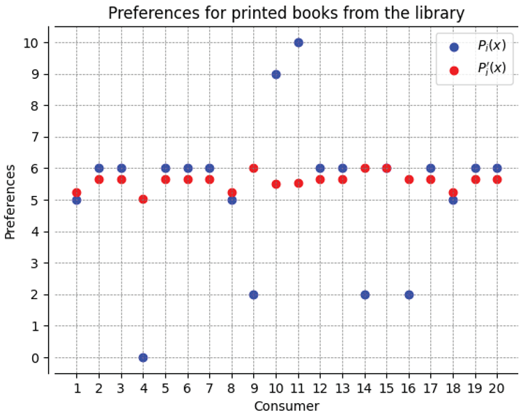
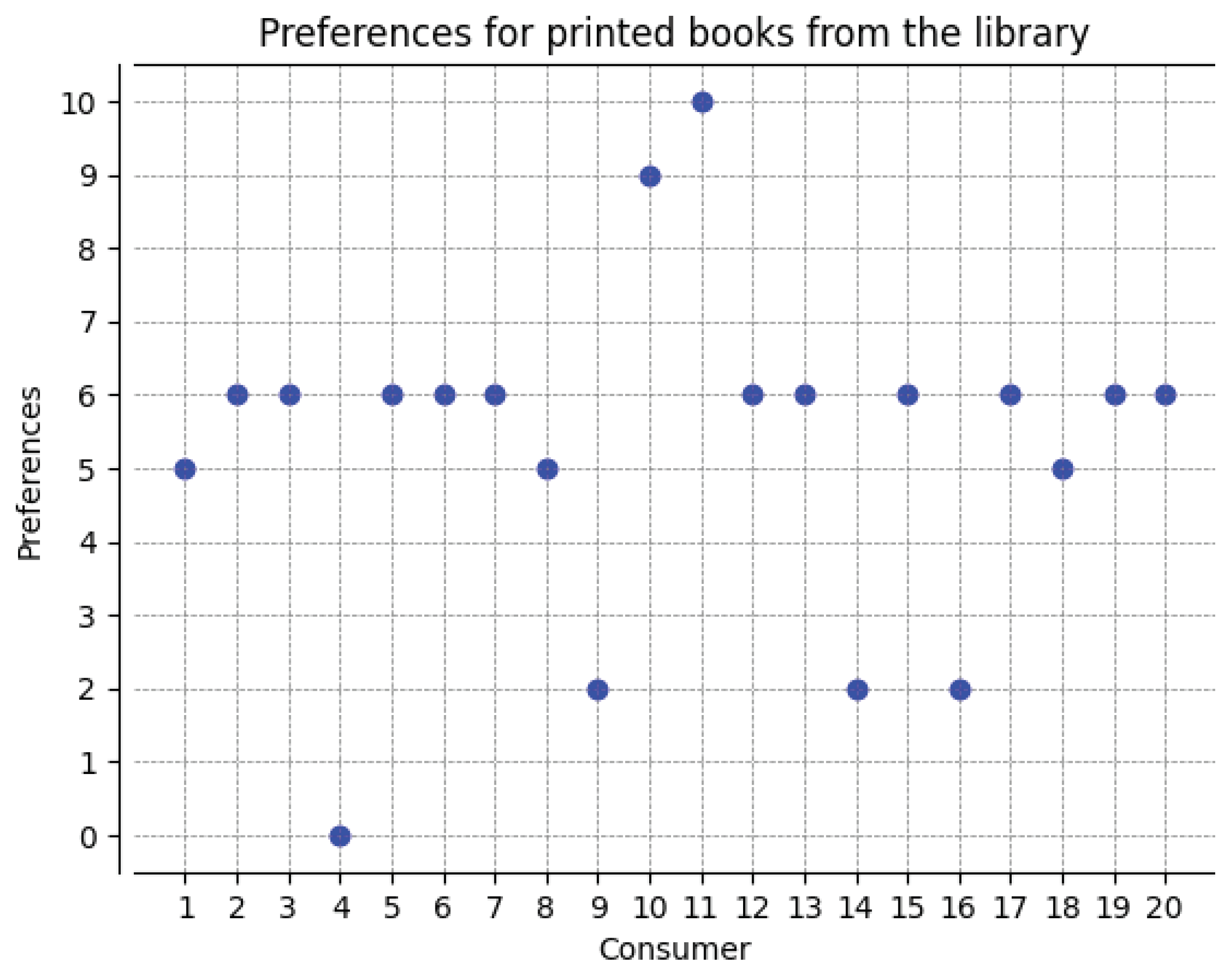
In the plot below (see Figure 1), we present declarations of 20 consumers, who have decided on the level of preferences for printed books from the library.

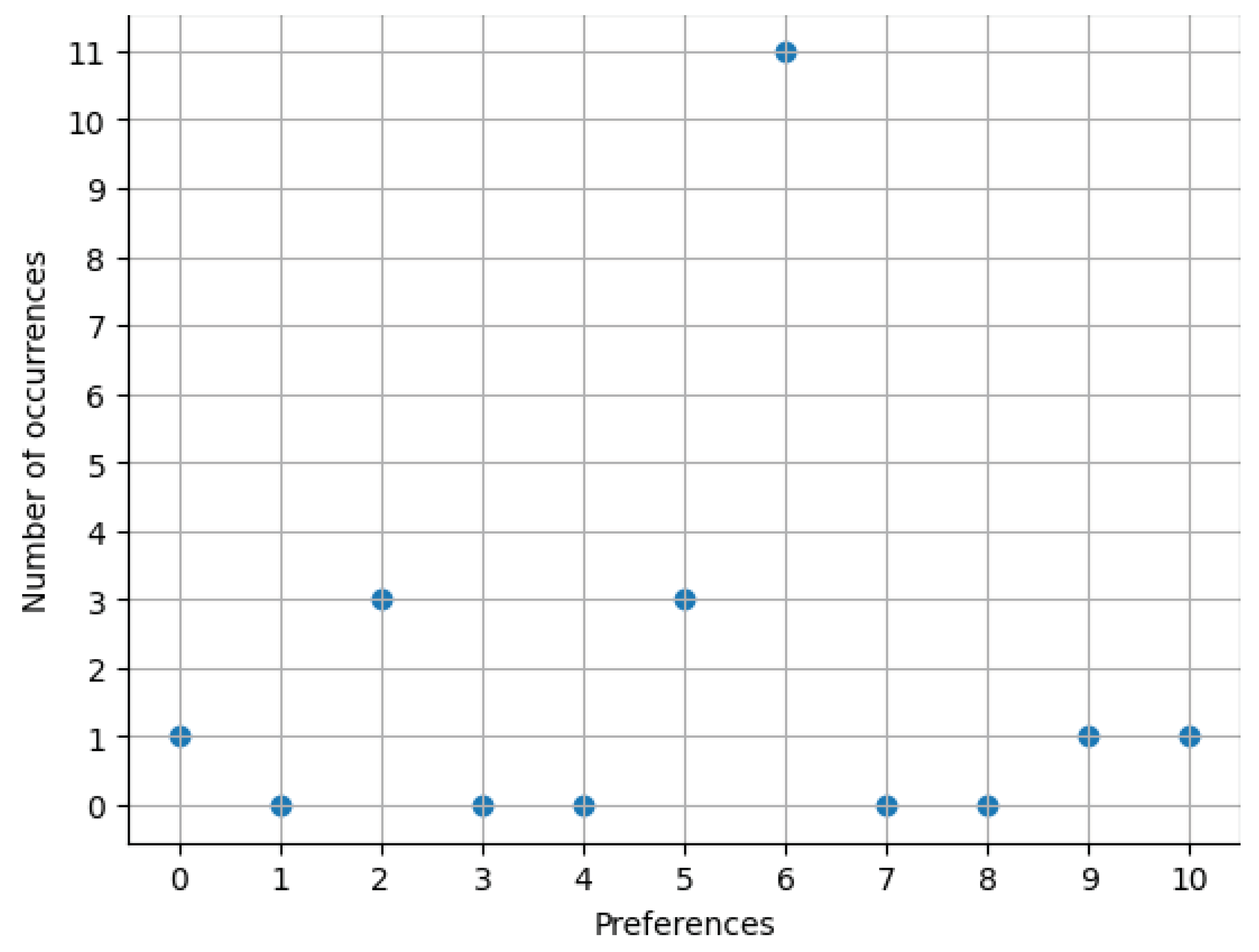
In the plot below (see Figure 2), we present the number of consumers based on their preference.

Indicating the values of preference weights based on the second plot (Figure 2): $W_0=\frac{1}{20}$, $W_2=\frac{3}{20}$, $W_5=\frac{3}{20}$, $W_6=\frac{11}{20}$, $W_9=\frac{1}{20}$ i $W_{10}=\frac{1}{20}$.

Let’s determine the value of social weight:

$S\left(x\right)=\frac{P_1^{\prime }\left(x\right)+...+P_n^{\prime }\left(x\right)}{n}=\frac{106}{10}=5,3$.

Let’s determine the value of individual preferences taking into account social preferences: $P_1^{\prime }\left(x\right)=5,25$, $P_2^{\prime }\left(x\right)\approx 5,66$, $P_4^{\prime }\left(x\right)\approx 5,04$, $P_9^{\prime }\left(x\right)\approx 6,01$, $P_{11}^{\prime }\left(x\right)\approx 5,54$ i $P_{10}^{\prime }\left(x\right)\approx 5,49$.

Now notice that the differences between individual preferences and preferences taking into account social factors:

In the analysis of differences between individual preferences and the combination of individual preferences with social ones dependent on social factors for various arguments, both positive and negative differences were observed. This suggests that the social influence on preferences is diverse and dependent on specific social context. This may be significant in decision-making contexts, especially when we want to understand which arguments are more susceptible to social influences. Analyzing cases with significant differences, for example for consumers 9, 10, 14, one may hypothesize that units with similar preferences characterized by higher social weight exert a greater influence on social preferences. For different arguments, the influence of social weight may vary, suggesting differences in how strongly social preferences depend on individual preferences depending on the social context. Differences between individual and social preferences may be more pronounced when the social average significantly differs from individual preferences. In cases where social preferences are more aligned with individual ones, it can be assumed that the social average reflects more dominant and accepted preferences in society.

Let $P_i,S:X\to Y$ and $P_i^{\prime }:[0,10]\times [0,1]\to Y$, where $Y=[0,m]$ for all $m\in {\mathbb{R}}_{+}$.

By analyzing the integral, where f represents the weight density function, with $\underset{0}{\overset{1}{\int }}f\left(W\right)dW=1$, we can observe how different values of social weight W contribute to the overall influence mass. This can provide information about whether there is a certain range of social weights that dominates in shaping social preferences. If $\underset{a}{\overset{b}{\int }}f\left(W\right)dW$ is close to ${\delta }_1$, we can interpret this as a limit of differentiation, indicating that we are analyzing the function f in the context of very small changes in W. This situation focuses on analyzing local changes in social weight and their impact on social preferences. It may be important to understand how small changes in social weight translate into the total social mass. This kind of approach can be used to find extrema of the function, where we analyze how very small changes in social weight affect changes in social preferences.

References

- Benhamouda, F., Bourse, F., Lipmaa, H., CCA-Secure Inner-Product Functional Encryption from Projective Hash Functions in: Lecture Notes in Computer Science. (s. 36-66). Cham: Springer International Publishing (2017). ISBN 978-3-319-70694-8.
- Boneh, D., Sahai, A., Waters, B., Functional Encryption: Definitions and Challenges, IACR, (2011), https://eprint.iacr.org/2011/543.pdf.
- Chambers, C., Echenique, F., Revealed Preference Theory, Cambridge: Cambridge University Press, (2016), ISBN 978-1-107-11971-9.
- Dryzek, J. S., Revealed Preference and the Pluralism of Rationality, Economics and Philosophy, 30 (3), (2014) 383-403.
- Manzini, P., Mariotti, M., Revealed Preference and Behavioral Economics, in Zamir, E., Teichman, D. (red.). The Oxford Handbook of Behavioral Economics and the Law, (2014), s. 3-21. Oxford: Oxford University Press. ISBN 978-0-19-994547-4.
- Samuelson, P. A., A note on the pure theory of consumers’ behaviour, Economica. New Series.5 (17): 61–71, 1938.
-
Azure Functions security, Microsoft Learn, (2022), https://docs.microsoft.com/en-us/learn/modules/secure-azure-functions/.