
Submitted:
20 March 2024
Posted:
21 March 2024
Read the latest preprint version here
Abstract
We describe a new approach for integrating multiple views of data into a common latent space using non-negative tensor factorization (NTF). This approach, which we refer to as the "Integrated Sources Model" (ISM), consists of two main steps: embedding and analysis. In the embedding step, each view is transformed into a matrix with common non-negative components. In the analysis step, the transformed views are combined into a tensor and decomposed using NTF. Noteworthy, ISM can be extended to process multi-view data sets with missing views. We illustrate the new approach using two examples: the UCI digit dataset and a public cell type gene signatures dataset, to show that multi-view clustering of digits or marker genes by their respective cell type is better achieved with ISM than with other latent space approaches. We also show how the non-negativity and sparsity of the ISM model components enable straightforward interpretations, in contrast to latent factors of mixed signs. Finally, we present potential applications to single-cell multi-omics and spatial mapping, including spatial imaging and spatial transcriptomics, and computational biology, which are currently under evaluation. ISM relies on state-of-the-art algorithms invoked via a simple workflow implemented in a Jupyter Python notebook.
Keywords:
Principal Component Analysis
; Non-negative Matrix Factorization
; Non-negative Tensor Factorization
; Multi-view Clustering
; Canonical Correlation Analysis
; Common Principal Components
; Multi Dimensional Scaling
1. Introduction
In machine learning, multi-view data involve multiple distinct sets of attributes (“views”) for a common set of observations. In the particular case where each view has the same attributes but is considered in a different context, the data is a multidimensional array of order 3 that can be thought of as a tensor. For example, an RGB image has three color channels: Red, Green and Blue, and each color channel is a two-dimensional matrix in which the intensity of the respective color is stored for each pixel. Non-negative Tensor Factorization (NTF) is a powerful latent space representation technique that is designed to analyze multidimensional arrays of order 3 or more. For example, color and spatial information of the image are captured by NTF non-negative factors, which can be used for various tasks such as image compression, enhancement, segmentation, classification and fusion [1].
Unfortunately, NTF cannot be applied to multi-view data when the views have heterogeneous content with distinct sets of attributes. For example, a text document can be mapped to different views, like Bag of Words, Topic Modeling, or Sentiment Analysis, each with a different set of attributes. Numerous algorithms have been proposed for this type of data, some of which have become popular in the machine learning community. For example, the MVLEARN package uses the Scikit-Learn API to make it easily accessible to Python users [2], and the Multi-Omics Factor Analysis (MOFA and MOFA+) Bioconductor packages [3,4] are widely used for the analysis of multi-omics datasets. However, because they assume a heterogeneous data structure, none of the algorithms implemented in these packages incorporate NTF's explicit factorization of a three-dimensional array. Other methods first convert each view into a similarity matrix between the observations. Since all views refer to the same observations, the similarity matrices have the same shape regardless of the view they come from, resulting in a tensor of similarity matrices. Multi-view clustering (MVC) is performed on these similarity matrices, sometimes using tensor-based approaches, such as Essential Tensor Learning for Multi-view Spectral Clustering or Multi-view Clustering via Semi-non-negative Tensor Factorization [5,6]. However, these clustering approaches cannot be applied to other tasks, such as data reduction. This is owing to the fact that the representations of such similarity matrices are not really a projection of the data from multiple views into a common latent space with a small number of common attributes, such as underlying factors or concepts.
In the context of heterogeneous views, we present in this article the Integrated Sources Model (ISM), which embeds each view into a common latent space using a sparse variant of Non-Negative Factorization (NMF). The embedded views having the same format constitute a three-dimensional array, which can be further analyzed by NTF. In addition to the NTF components, a view-mapping matrix is estimated to obtain an interpretable link between the dimensions of the latent space and the original attributes from each view.
ISM belongs to the class of multi-view Latent Space representation methods. Approaches such as Consensus PCA, Stepwise Common Principal Components (Stepwise CPCs), Generalized Canonical Correlation Analysis (GCCA), Latent Multi-view Subspace Clustering and Multi-View Clustering in Latent Embedding Space [7,8,9,10,11], Group Factor Analysis (GFA) [12,13], Regularized Multi-Manifold NMF [14], to name just a few, try to capture underlying factors or concepts that characterize the data in the latent space while filtering out noise and redundancy. For MVC applications, performing cluster analysis in the latent space generally results in more accurate and consistent cluster partitioning [15]. It is noteworthy that these approaches allow newly collected data (i.e. data that is not part of the data used to train/learn the model) to be embedded in the latent space, and thus are not limited to the purpose of multi-view clustering.
Compared to the above approaches, the originality of ISM lies in its simple workflow involving NMF and NTF steps. As a result, ISM also produces latent factors whose interpretation is greatly facilitated by the non-negativity of the attribute loadings that define them, since they cannot cancel each other out. In a clinical study comprising several surveys with heterogeneous content, for example, the interpretability of latent factors is of critical importance if they are to be used by an investigator as a follow-up tool. In addition, ISM benefits directly from the proven performance and convergence properties of the NMF and NTF algorithms, whose availability in the form of powerful Python or R packages ensures scalability and accessibility for the vast majority of the machine learning community.
2. Materials and Methods
2.1. Materials
UCI Digits Data: The data can found at Datasets - Datasets - UCI Machine Learning Repository and contains 6 heterogenous views: 76 Fourier coefficients of the character shapes, 216 profile correlations, 64 Karhunen-Love coefficients, 240 pixel averages of the images from 2x3 windows, 47 Zernike moments and 6 morphological features, where each class contains 200 labeled examples.
Signature 915 Data: The data can be found at https://academic.oup.com/bioinformatics/article/38/4/1015/6426077#supplementary-data in supplementary table S4 (list of 915 marker genes and corresponding cell types) and GEO Accession viewer (nih.gov) (expression data). In 4 views corresponding to different patients, the expressions of 915 marker genes are measured across 16 different cell-types. In other words, this dataset contains 4 views of the 915 gene markers (one view per patient) measured in 16 different cell-types.
2.1. Methods
Outline of ISM and comparison with other Latent Space approaches
Before delving into the details of the ISM workflow, let's introduce the main underlying ideas with an illustrative figure (Figure 1, panel A) and try to compare with other Latent Space approaches (Figure 2, panel B). The different views are represented by heatmaps on the left side of both panels, with attributes on the vertical axis and observations on the horizontal axis, respectively.
- ISM (Figure 1A):
In the central part of the figure, each view has been decomposed into the product of two matrices and using NMF. Each matrix corresponds to the transformation of a particular view to a latent space that is common to all transformed views. ISM ensures that the transformed views share the same number and type of latent attributes, called components, as explained in the detailed description. This transforming process, which we call embedding, results in a three-dimensional array, or tensor. The corresponding matrices contain the loadings of the original attributes on each component. We call these matrices the mapping between the original and transformed views.
In the right part of the figure, the three-dimensional array is decomposed into the tensor product of three matrices: using NTF. contains the meta-scores – the single transformation to the latent space common to all views. and contain the loadings of NMF latent attributes and views, respectively, on each NTF component. Each row of is represented by a diagonal matrix, where the diagonal contains the loadings for a particular view. This allows, for each view of the tensor, to translate in the figure the tensor product into a simple matrix product .
Other Latent Space approaches (Figure 1B):
In the right part of the figure, each view has been decomposed into the product of two matrices and using the latent space method algorithm. As with ISM, contains the meta-scores – the single transformation in the latent space common to all views.
- Comparison between ISM and other Latent Space approaches:
If we multiply in Figure 1A each mapping matrix by , we obtain a representation that is similar to Figure 1B. This shows that ISM belongs to the family of Latent Space decomposition methods. However, view loadings are a constitutive part of ISM, whereas they are derived in other models, e.g. using variance decomposition by factor as in the MOFA article [3].
- Detailed workflows
In this section, we present three workflows. The first workflow consists of training the ISM model to generate a latent space representation and view-mapping. The second workflow enables the projection of new observations obtained in multiple views into the latent space. The third workflow contains the detailed analysis steps for each example.
Workflow 1: Latent Space Representation and View-Mapping
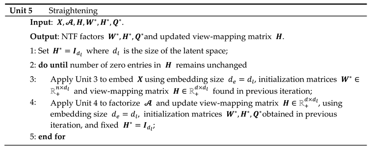
The training of the ISM model can be divided into 5 units as described in figure 2. The first 4 process units enable the discovery of the latent space in an “embedding” space. Once the latent space has been found, it is assimilated with the embedding space. During the fifth "straightening" unit, the latent space remains fixed, while the sequence of units 3, 4 and 2 is repeated to further parsimonize the view-mapping until the degree of sparsity remains unchanged. The sizes of the embedding space and the latent space are discussed in the section describing the third workflow.
- Unit 1: Initialization
A non-negative matrix factorization is first performed on the matrix of the concatenated views , resulting in the decomposition: where represents the transformed data, the columns of contain the loadings of the attributes across all views on each component, is the embedding size and is the total number of observations.
- Unit 2: Parsimonization
The initial degree of sparsity in is crucial to the embedding dimensions from being overly distorted between the different views during the embedding process, as will be seen in the next section. This is achieved by applying a hard-threshold to each column of the matrix. The threshold is based on the reciprocal of the Herfindhal-Hirschman index [16], which provides an estimate of the number of non-negligible values in a non-negative vector. For columns with strongly positively skewed values, the use of the L2 norm for the estimate’s denominator can lead to excessively sparse factors, which in turn can lead to an overly large approximation error during embedding. Therefore, the estimate is multiplied by a coefficient whose default value was set at 0.8 after extensive testing with various data sets.
- Unit 3: Embedding
and are further updated along each view, yielding matrices of common shape (number of observations factorization rank ) corresponding to the transformed views.
NMF multiplicative updates are used during view matching to leave the zeros in the primary matrix unchanged. Further optimizations of the simplicial cones for each view are therefore limited to the non-zero loadings so that they remain tightly connected. This ensures that the transformed views form a tensor. Multiplicative updates usually start with a linear rate of convergence, which becomes sublinear after a few hundred iterations [17]. By default, the number of iterations is set to 200 to ensure a reasonable approximation to each view, as required for the latent space representation described in the next section.
- Unit 4: Latent space representation and view-mapping
The resulting tensor is analyzed using NTF, which leads to the decomposition: where and is the dimension of the latent space. The components , and enable the reconstruction of the horizontal, lateral and frontal slices of the embedding tensor: the loadings of the views on each component are contained in the matrix ; the integrated multiple views, or meta-scores, are contained in the matrix ; and the matrix represents the latent space in the form of a simplicial cone contained in the embedding space. Finally, the view-mapping matrix is updated by applying steps 3-8 of unit 4. Its sparsity is ensured by further applying the parsimonization unit 2.
- Unit 5: Straightening
The sparsity of the view-mapping matrix can be further optimized together with the meta-scores and the view-loadings by repeating units 3, 4 and 2 until the number of 0-entries in remains unchanged. To achieve this, the embedding is restricted to the latent space defined by the simplicial cone formed by . In this simplified embedding space, becomes the Identity matrix when the updating process of and starts. In other words, embedding and latent spaces are being assimilated during the straightening process. Optionally, for faster convergence, can be fixed to , at the cost of a slightly higher approximation error, as observed in numerous experiments, due to only small deviations from .
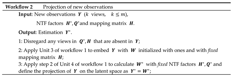
Workflow 2: Projection of New Observations
For new observations comprising views, , ISM parameters , and view-mapping matrix can be used to project on the latent ISM components, as described in workflow 2.
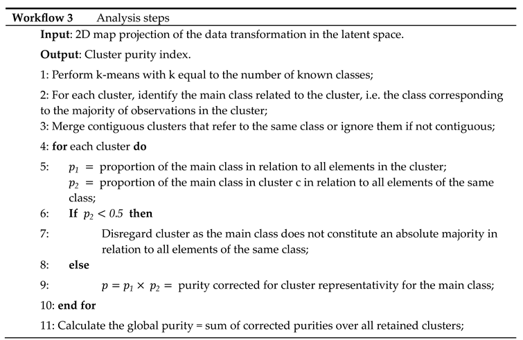
Workflow 3: Data Analysis
The data from the UCI Digits and Signature 915 datasets are analyzed using several alternative approaches: ISM, Multi-View Multi-Dimensional Scaling (MVMDS), NMF, NTF and Principal Components Analysis (PCA). Because PCA and NMF are not multi-view approaches, they are applied to the concatenated views. To facilitate interpretation, the transformed data is projected onto a 2D map before being subjected to k-means clustering, where k is the known number of classes (k-means clustering was chosen for its versatility and simplicity, as it only requires the number of clusters to be found, and this number is known in both our example datasets). Within each cluster, the class that contains the majority of the points, i.e. the main class, is identified. If two clusters share the same main class, they are merged, unless they are not contiguous (ratio of the distance between the centroids to the intra-cluster distance between points > 1). In this case, the non-contiguous clusters are excluded because they are assigned to the same class, which should appear homogeneous in the representation. Similarly, any cluster that does not contain an absolute majority is not considered clearly representative of the class to which it is assigned and is excluded. A global purity index is then calculated for the remaining clusters. To enhance clarity, the clusters are visualized using 95% confidence ellipses, while the classes are represented using as distinct colors as possible.
Multidimensional scaling (MDS) is applied to the 2D map projection. MDS uses a simple metric objective to find a low-dimensional embedding that accurately represents the distances between points in the latent space [18]. MDS is therefore agnostic to the intrinsic clustering performances of the methods that we want to evaluate. Effective embedding methods, e.g., UMAP or t-SNE, are not as optimal for preserving the global geometric structure in the latent space [19]. For example, a resolution parameter needs to be defined for the UMAP embedding of single-cell data, whereby a higher resolution leads to a higher number of clusters. In addition, the subtle differences between some cell types from one family can be smoothed out if the dataset contains transcriptionally distinct cell types from multiple families, as is the case with immune cells (second dataset in the article).
Latent Space methods require that the rank of the factorization is determined in advance. ISM benefits from the advantages of the NMF and NTF components, i.e. the choice of the correct rank is less critical than with other methods (we will come back to this point in the Results and Discussion). This allows, even if we expect some redundancy in the latent factors due to the proximity of certain digits or cell types, to set the rank to the number of known classes. However, the dimension of the ISM embedding space must also be determined during the discovery step. The choice of close dimensions for the embedding and latent spaces is consistent with the fact that both spaces are merged at the end of the ISM workflow. Thus, we examine the approximation error for an embedding dimension in the neighborhood of the chosen rank. The rank for PCA and MVMDS is set by inspecting the screeplot of the variance ratio.
The analysis of the Signature 915 data also examines the biological relevance of the distance between clusters in each latent multi-view space.
Detailed analysis steps are provided in workflow 3.
3. Results
Workflow 3 contains detailed calculation steps for the purity index; it was applied on the two datasets.
3.1. UCI Digits Data
PCA and MVMDS use a 10-factorization rank. ISM uses a primary embedding of dimension 9 and a 10-factorization rank. The clusterings of the digits along ISM, Multi-View Multi Dimensional Scaling (MVMDS), NMF and PCA components are shown in 2D scatterplots of the MDS projection of transformed data (Figure 3). The Karhunen-Love coefficients contain data with mixed signs, so the corresponding view is split into its positive part and the absolute value of its negative part when applying the non-negative approaches ISM and NMF. The clustering based on the application of MDS on the concatenated views is also shown. A k-means clustering with 10 classes is performed for each approach to identify digit-specific clusters containing an absolute majority of a given digit. ISM is the only method that separates the 10 classes of digits, with some of the classes forming isolated clusters, and with a higher purity index than all other competing approaches except NMF, which gives a slightly higher index than ISM (5.84 versus 5.81, Table 1). However, the digits 5 and 3 are mixed together so that one less digit is recognized. This illustrates the complementarity between the number of recognized classes and the purity index. Figure 4 shows how the views affect the individual ISM components by using a treemap chart. For each component, each view corresponds to a rectangle within a rectangular display, where the size of the rectangle represents the loading of the view. It is noteworthy that some components are only supported by a few views, e.g., component 1 (2 views) and 8 (3 views), while others involve most views, e.g., component 5 (6 views). As each component is associated with a digit, this emphasizes the specifics and complementarity of the image representations that are dependent on the respective digit. It is also interesting to note that for some components, the loadings of the views are diametrically opposed to the respective number of attributes, e.g. for component 8 the view of 240 pixel averages has the lowest loading, while the view of 6 morphological features has the highest loading. This clearly shows that the views are evenly balanced regardless of their respective number of attributes when using ISM.
3.2. Signature 915 Data
Prior to the analysis, each marker gene was normalized using the mean of the 4 highest expression values corresponding to the mean expression in the respective cell-type. PCA and MVMDS use a 10-factorization rank. ISM uses a primary embedding of dimension 16 and a 16-factorization rank. The clusterings of the marker genes along ISM, MVMDS, NMF, NTF and PCA components are shown in 2D scatterplots of the MDS projection of the transformed data (Figure 5). A k-means clustering with 16 classes is performed for each approach to identify cell type-specific clusters containing an absolute majority of the marker genes of a given cell type. ISM outperforms the other methods with 14 cell type-specific clusters, and with a higher purity index than any other approach (Table 2). As seen in the example of the UCI digits, the NMF purity index is close to the ISM index (11.24 versus 11.46). However, the naïve B cells are divided into two groups on either side of the neutrophil LD cells, resulting in one less cell type being recognized.
Regarding the positioning of the clusters on the 2D map, MVMDS places monocyte C and monocyte NC+I opposite of each other, contrary to all other approaches and, more importantly, against biological intuition. The ISM method outperforms other methods on this dataset as it reveals a tight proximity between transcriptionally and functionally close cell types of the major immune cell families. Indeed, three cell types from the myeloid lineage, including monocytes C, monocytes NC+I and mDC, were grouped together. The same trend is observed for three cell types from the B cell family, where only ISM revealed close proximity of naïve B cells, memory B cells and plasmablasts, out of the five methods considered. The most challenging cell types were in the T cell family, where ISM was able to identify clusters for three cell types (CD4+ effectors, naïve T cells and VD+ gamma delta non-conventional T cells) and place them in close proximity. VD+ gamma delta non-conventional T cells have also some similarities with NK cells in terms of expression of some receptors, and only the ISM method was able to recognize both cell types and place them in close proximity to reveal their similarity. The ISM method was also able to capture some other subtle similarities between two types of dendritic cells, mDC and pDC, which correspond to antigen-presenting cells.
Figure 6 shows how the 4 patients impact the individual ISM components by using a treemap chart. For each component, each patient corresponds to a rectangle within a rectangular display, where the size of the rectangle represents the loading of the patient. In contrast to the UCI digits data, most components are supported by 3 patients (3 components) or 4 patients (11 components). Two components involve only 2 patients.
The loadings of the view-mapping matrix are shown in Figure 7 by using a treemap chart. Recall that each attribute of this dataset is a combination of a patient and a cell-type, in which the expressions of 915 marker genes were measured. For each component, such a combination corresponds to a rectangle within a rectangular display, where the size of the rectangle represents the loading of the combination. ISM components 1 and 2 are both associated with the same cell type pDC, while component 15 is simultaneously associated with CD8-activated, VD2- and VD2+ cells. In the final clustering, the cluster comprising these 3 cell types has no main type and is therefore discarded, resulting in 13 identified cell-types.
3.3. Further Insights Regarding the Model
Model's Potential Dependency on Input Parameterization
In this section, we evaluate how ISM performance might be affected by changing the embedding dimension and the rank in the neighborhood of the chosen values. First, we examine the relative approximation error for an embedding dimension in the neighborhood of the chosen rank, in order to select an optimal value, as described in the analysis workflow. Second, we examine the relative error, number of found classes and purity for a rank in the neighborhood of the chosen embedding dimension.
For the UCI digits data, where the chosen ISM rank is 10, an embedding dimension of 9 clearly minimizes the relative error: 0.52 versus 0.72 or higher for other dimensions. The number of classes found and the purity index are also significantly higher (Table 3, upper part). The relative error associated with a rank is not as critical if it exceeds the number of known classes: Compared to a 10-rank ISM model, a 12-rank model also finds 10 classes and gives a slightly higher purity index: 6.24 versus 5.81, despite a larger relative error: 0.60 versus 0.52 (Table 3, bottom part). The next section discusses this point further.
For the Signature 915 data, where the chosen ISM rank is 16, the relative error does not change significantly for neighboring embedding dimensions: 0.33 for a 15-embedding and 0.34 for a 17-embedding (Table 4, upper part). Choosing an embedding dimension equal to the rank is more consistent with the ISM workflow, where embedding and latent spaces are united during the straightening process. Therefore, we chose an embedding dimension of 16. In terms of purity, a 17-rank ISM model gives results that are slightly superior to the 16-rank ISM model (Table 4, bottom part).
Overall, these results tend to confirm that ISM provides relatively stable estimates in the neighborhood of the chosen rank, in line with its parent methods NMF and NTF.
Evolution of the Relative Error over the Course of Model Training
In this section, we evaluate how each main factorization step performed in the ISM workflow contributes to the final approximation error. Specifically, we examine the relative error obtained after (i) the preliminary NMF, (ii) the first call to NTF prior to the straightening process, and (iii) the last iteration of NTF in the straightening process.
While the increase in relative error is very small for the Signature 915 data (0.35 versus 0.30), we observe a large increase for the UCI digit data (0.53 versus 0.36). This increase is mainly due to the straightening process (0.53 versus 0.39 before). Recall that this process iteratively parsimonizes the view-mapping matrix . The very sparse nature of the Signature 915 data explains the difference in behavior between the two datasets: For the denser UCI digit data, the increased sparsity of the view-mapping matrix induced by the straightening process significantly inflates the relative error, as more of the smaller values in the original views are filtered out. Unless the zero attribute loadings in some of the ISM components are relevant to digit class identification, this is not an issue. In fact, if we bypass the straightening process to achieve a smaller relative error, the performance of ISM is reduced: Only 9 digit classes are found instead of 10, and the purity is 5.45 instead of 5.81, indicating that the model becomes overfit. This illustrates how ISM manages to filter out the specific part of the signal that is irrelevant to the main mechanisms in the data and hinders their recovery.
4. Discussion
The performance metrics used with our two example datasets show that ISM performs as well as or better than other methods. The fact that the ISM workflow uses algorithms with proven performance and convergence properties, such as NMF and NTF, is consistent with the good performance of ISM observed in our examples.
To our knowledge, ISM is the first approach that uses NMF to transform heterogeneous views into a three-dimensional array and then uses NTF to extract consistent information from the transformed views. Just as NMF and NTF factors are more interpretable and meaningful because they cannot cancel each other out due to the non-negativity of their loadings, ISM produces latent factors whose interpretation is greatly facilitated by the non-negativity of the attribute loadings that define them, as illustrated by the example of the Signature 915 data.
Sparsity is an important element of the ISM workflow, which further facilitates the interpretation of latent factors. Noteworthy, no parameter for sparsity needs to be defined, as the hard threshold calculation for latent factors is automatically selected as the reciprocal of the Herfindhal-Hirschman index. However, for factors with strongly positively skewed values, the use of the L2 norm for the denominator of the index can lead to excessively sparse factors, which in turn can lead to an overly large approximation error during embedding. Therefore, this threshold can be scaled down by a multiplicative factor to achieve a better mapping to each view, which can lead to greater consistency in the analysis, as long as the intrinsic nature of the embedding tensor is preserved, i.e. the embedding dimensions remain comparable in the different views. In our workflow implementation, the default value for the multiplicative factor was set to 0.8 after extensive testing with various data sets.
As with all factorization methods, the factorization rank must be determined in advance. However, non-negative factorization-based methods, including ISM, are not subject to orthogonality constraints and can therefore create a new dimension by, for example, splitting a given component into two parts to disentangle close mechanisms that are otherwise intertwined in that component [20]. Finding the correct rank is therefore less critical than with mixed signed factorization approaches such as SVD, where low variance components tend to represent the noisy part of the data. However, multiple solutions have been proposed, among which the cophenetic correlation coefficient, which is widely used to estimate a rank that provides the most stable clustering derived from the NMF components [21]. A similar criterion, named concordance has been proposed in [22], where extensive simulations showed that NMF finds the most stable solutions around the correct rank, even if the latent factors are strongly correlated. While such approach could be used with ISM to determine the best combination for the preliminary embedding and latent space dimensions, it would become too greedy. However, in line with the fact that embedding and latent spaces are later merged in the ISM workflow, it can still be applied in the case where the model imposes the same dimensions for both parameters. Next, as was done in the analysis of our examples, the embedding dimension can be further optimized by examining the approximation error in the neighborhood of the chosen rank.
Redundancy in the latent factors is also a problem for NMF-based techniques, as identified and illustrated early on with Donoho's swimmer data set, where a ghost torso was found in all basis vectors representing the body parts with different orientations [23]. L1 regularization techniques, e.g. using Hoyer’s sparsity index [24,25] or appropriate initialization such as Non-Negative SVD (NNSVD) [26] can help to mitigate these problems. Of note, in our ISM workflow implementation, the Herfindhal-Hirschman index used in the embedding step is mathematically equivalent to the Hoyer sparsity index, and NNSVD is used for NMF and NTF initialization.
ISM intrinsic view loadings also enable the automatic weighting of the views within each latent factor. This allows the simultaneous analysis of views of very different sizes without the need for prior normalization to give each view the same importance, as is the case with Consensus PCA, for example.
Recently, graph transformers and deep learning approaches have been proposed for the inference of biological single-cell networks [27]. The preliminary NMF in Unit 1 of Workflow 1, which combines the data prior to the application of NTF, is in a way reminiscent of the 'attention' mechanism used in transformers prior to the application of a lightweight neural network [28]. This could explain why ISM can outperform NTF when applied to a multidimensional array, i.e. even if the data structure is suitable for the direct application of NTF, as shown by the clustering of marker genes achieved in the application example. This could also explain why, although NMF performance is close to ISM performance in terms of the purity index, ISM outperforms NMF in both examples in terms of number of recognized classes and, in the second example, by generating a better positioning of recognized cell types on the 2D map projection.
Like other latent space methods, ISM is not limited to the purpose of multi-view clustering. The ISM components, as well as the view-mapping matrix, can be used for data reduction on newly collected data (i.e. data that is not part of the data used to train/learn the model) by fixing these components in the ISM model. Data reduction for newly collected data is still feasible even if some of the views contained in the training data are missing, as the ISM parameters are compartmentalized by view.
ISM is not limited to views with non-negative data. Each mixed-signed view can be split into its positive part and the absolute value of its negative part, resulting in two different non-negative views, as illustrated in the UCI digits data example.
An important limitation of ISM and of other multi-view latent space approaches is the required availability of multi-view data for all observations in the training set. For financial or logistical reasons, a particular view may be missing in a subset of the observations, and this subset is in turn dependent on the view under consideration. We are currently evaluating a variant of ISM that can process multi-view data with missing views. In this approach, sets of views that have enough common observations are integrated with ISM separately. By using the model parameters, the transformation into the latent ISM space can be expanded to all views over all observations belonging to the set, resulting in much larger transformed views than the original intersection would allow. This expansion process enables the integration of the ISM-transformed data from the different view sets, again using the ISM. For this reason, we call this variant the Integrated Latent Space Model, ILSM. Interestingly, a similar integrated latent space approach has already been proposed to study the influence of social networks on human behavior [29]. After masking a large number of views, the dataset of UCI digits was analyzed using ILSM. A more detailed description of the expansion process (Workflow S1, Figure S1) and promising results (Figure S2) can be found in the supplementary materials.
5. Conclusion
To illustrate the key benefits of ISM, we present some potential applications that are currently being evaluated and the results of which will be published in future articles.
In longitudinal clinical studies, where participants are followed up later in the study, the ISM model can be trained at baseline and applied to subsequent data to calculate meta-scores. The fact that the associated components are fully interpretable increases the appeal of ISM meta-scores to clinicians, in contrast to mixed-sign latent factors provided by other factorization methods.
Let’s consider complex multidimensional multi-omics data from one and the same set of cells (single cell technology). In fact, there is a growing amount of single-cell data corresponding to different molecular layers of the same cell. Data integration is a challenge as each modality can provide a different clustering stemming from a specific biological signal. Therefore, data integration and its projection into a space must (i) preserve the consensus between two clusterings and (ii) highlight the differences that each modality may bring. The ISM view loadings can address these two key requirements: Components with similar contributions from each molecular layer highlight a consensus that can be inferred from the clustering based on the ISM meta-scores of such components. In contrast, components with differing contributions from each molecular layer highlight the specificities of each modality, which can be inferred from the clustering based on the ISM meta-scores of such components.
The area of spatial mapping, including spatial imaging and spatial transcriptomics, is expanding at an unprecedented pace. An effective method for integrating different levels of information such as gene or protein expression and spatial organization of cell phenotypes is an unmet methodological need. We believe that ISM can integrate these different levels of information, as shown in the analysis of the UCI digits data, to capture the constituents that allow spatial patterns to be distinguished across all levels.
The identification of new chemotypes with biological activity which is similar to that of a known active molecule is an important challenge in drug discovery known as "scaffold hopping" [30]. In this context, we are currently analyzing the fingerprints of the docking of tens of thousands of molecules to dozens of proteins, with protein-associated fingerprints forming the different views of each molecule. The goal is to use the ISM-transformed fingerprints to predict scaffold-hopping chemotypes. Given the enormous size of the dataset – each fingerprint contains more than 100 binary digits – the ILSM strategy is being evaluated as a possible way to reduce computational problems, as smaller sets of views can be analyzed on smaller subsets of observations before integrating them in their entirety.
6. Implementation
For k-means, MDS and PCA, Scikit-learn [31] was used. The mvlearn package was used for MVMDS.
NMF and NTF were performed with the package adnmtf.
ISM is implemented in Python and is invoked from a Jupyter Python notebook available on the Advestis GitHub. (Advestis part of Mazars · GitHub)
Matplotlib, Pyplot tutorial — Matplotlib 3.8.2 documentation was used to create the clustering figures.
Treemaps were obtained with the Graph Builder platform from JMP®, Version 17.2.0. SAS Institute Inc., Cary, NC, 1989–2023.
The distinctipy package was used to generate colors that are visually distinct from one another.
Figure 1 was created using elements provided by Servier Medical Art (Citation & Sharing - Servier Medical Art).
7. Patents
Paul Fogel has filed a Provisional Application: US 63/616,801 under 35 USC 111(b) with the United States Patent and Trademark Office (USPTO) under the title “THE INTEGRATED SOURCES MODEL: A GENERALIZATION OF NON-NEGATIVE TENSORFACTORIZATION FOR THE ANALYSIS OF MULTIPLE HETEROGENEOUS DATA VIEWS.”
Supplementary Materials
The following supporting information can be downloaded at the website of this paper posted on Preprints.org, Figure S1: ILSM analysis of the UCI digits data with masked views.
Author Contributions
Conceptualization: P.F. and G.L.; methodology, software and visualization: P.F.; writing—original draft preparation, P. F., C.G. and G.B; writing—review and editing: F.A., C.G and G.L.; investigation: G.B. and F.A. All authors have read and agreed to the published version of the manuscript.
Funding
This research received no external funding.
Data Availability Statement
The data used in this article and the ISM Jupyter python notebook can be downloaded from the Advestis part of Mazars GitHub repository.
Acknowledgments
Our sincere thanks to Prasad Chaskar, Translational Medicine Senior Expert Data Science Lead at Galderma, for stimulating discussions, especially on potential limitations arising from missing views when training latent models with multiple views; to Philippe Pinel, Center for Computation Biology, Mines Paris/PSL and Iktos SAS, Paris France, for discussions on addressing ISM calculation challenges in Computational Biology.
Conflicts of Interest
The authors declare no conflicts of interest.
References
- Cichocki, A., Zdunek, R., Phan, A., & Amari, S. (2009). Nonnegative Matrix and Tensor Factorizations - Applications to Exploratory Multi-way Data Analysis and Blind Source Separation. IEEE Signal Processing Magazine, 25, 142-145.
- Perry, R., Mischler, G., Guo, R., Lee, T.V., Chang, A., Koul, A., Franz, C., & Vogelstein, J.T. (2020). mvlearn: Multiview Machine Learning in Python. ArXiv, abs/2005.11890.
- Argelaguet, R., Velten, B., Arnol, D., Dietrich, S., Zenz, T., Marioni, J.C., Buettner, F., Huber, W., & Stegle, O. (2018). Multi-Omics Factor Analysis—a framework for unsupervised integration of multi-omics data sets. Molecular Systems Biology, 14. [CrossRef]
- Argelaguet, R., Arnol, D., Bredikhin, D., Deloro, Y., Velten, B., Marioni, J.C., & Stegle, O. (2020). MOFA+: a statistical framework for comprehensive integration of multi-modal single-cell data. Genome Biology, 21. [CrossRef]
- Wu, J., Lin, Z., & Zha, H. (2018). Essential Tensor Learning for Multi-View Spectral Clustering. IEEE Transactions on Image Processing, 28, 5910-5922. [CrossRef]
- Li, J., Gao, Q., Wang, Q., Xia, W., & Gao, X. (2023). Multi-View Clustering via Semi-non-negative Tensor Factorization. ArXiv, abs/2303.16748.
- Smilde, A.K., Westerhuis, J.A., & de Jong, S. (2003). A framework for sequential multiblock component methods. Journal of Chemometrics, 17. [CrossRef]
- Trendafilov, N.T. (2010). Stepwise estimation of common principal components. Comput. Stat. Data Anal., 54, 3446-3457. [CrossRef]
- Tenenhaus, A., & Tenenhaus, M. (2013). Regularized generalized canonical correlation analysis for multiblock or multigroup data analysis. Eur. J. Oper. Res., 238, 391-403. [CrossRef]
- Zhang, C., Hu, Q., Fu, H., Zhu, P.F., & Cao, X. (2017). Latent Multi-view Subspace Clustering. 2017 IEEE Conference on Computer Vision and Pattern Recognition (CVPR), 4333-4341.
- Chen, M., Huang, L., Wang, C., & Huang, D. (2020). Multi-View Clustering in Latent Embedding Space. AAAI Conference on Artificial Intelligence.
- Leppäaho, E., Ammad-ud-din, M., & Kaski, S. (2016). GFA: Exploratory Analysis of Multiple Data Sources with Group Factor Analysis. J. Mach. Learn. Res., 18, 39:1-39:5.
- Zhao, S., Gao, C., Mukherjee, S., & Engelhardt, B.E. (2016). Bayesian group factor analysis with structured sparsity. J. Mach. Learn. Res., 17, 196:1-196:47.
- Zhang, X., Zhao, L., Zong, L., Liu, X., & Yu, H. (2014). Multi-view Clustering via Multi-manifold Regularized Nonnegative Matrix Factorization. 2014 IEEE International Conference on Data Mining, 1103-1108. [CrossRef]
- Fu, L., Lin, P., Vasilakos, A.V., & Wang, S. (2020). An overview of recent multi-view clustering. Neurocomputing, 402, 148-161. [CrossRef]
- Hirschman, A.O. (1964). The Paternity of an Index. The American Economic Review, 54, 761-762.
- Badeau, R., Bertin, N., & Vincent, E. (2010). Stability Analysis of Multiplicative Update Algorithms and Application to Nonnegative Matrix Factorization. IEEE Transactions on Neural Networks, 21, 1869-1881. [CrossRef]
- Demaine, E.D., Hesterberg, A., Koehler, F., Lynch, J., & Urschel, J.C. (2021). Multidimensional Scaling: Approximation and Complexity. International Conference on Machine Learning.
- Zhai, Z., Lei, Y.L., Wang, R., & Xie, Y. (2022). Supervised capacity preserving mapping: a clustering guided visualization method for scRNA-seq data. Bioinformatics, 38, 2496 - 2503. [CrossRef]
- Fogel, P., Hawkins, D.M., Beecher, C., Luta, G., & Young, S.S. (2013). A Tale of Two Matrix Factorizations. The American Statistician, 67, 207 - 218. [CrossRef]
- Brunet, J., Tamayo, P., Golub, T.R., & Mesirov, J.P. (2004). Metagenes and molecular pattern discovery using matrix factorization. Proceedings of the National Academy of Sciences of the United States of America, 101, 4164 - 4169.
- Fogel, P., Geissler, C., Morizet, N., & Luta, G. (2023). On Rank Selection in Non-Negative Matrix Factorization Using Concordance. Mathematics. [CrossRef]
- Donoho, D.L., & Stodden, V. (2003). When Does Non-Negative Matrix Factorization Give a Correct Decomposition into Parts? Neural Information Processing Systems.
- Hoyer, P.O. Non-negative matrix factorization with sparseness constraints. J. Mach. Learn. Res. 2004, 5, 1457–1469. [CrossRef]
- Potluru, V.K., Plis, S., Le Roux, J., Pearlmutter, B.A., Calhoun, V.D., & Hayes, T.P. (2013). Block Coordinate Descent for Sparse NMF. CoRR, abs/1301.3527.
- Boutsidis, C.; Gallopoulos, E. SVD based initialization: A head start for nonnegative matrix factorization. Pattern Recognit. 2008, 41, 1350–1362. [CrossRef]
- Ma, A., Wang, X., Li, J., Wang, C., Xiao, T., Liu, Y., Cheng, H., Wang, J., Li, Y., Chang, Y., Li, J., Wang, D., Jiang, Y., Su, L., Xin, G., Gu, S., Li, Z., Liu, B., Xu, D., & Ma, Q. (2023). Single-cell biological network inference using a heterogeneous graph transformer. Nature Communications, 14. [CrossRef]
- Vaswani, Ashish, Noam M. Shazeer, Niki Parmar, Jakob Uszkoreit, Llion Jones, Aidan N. Gomez, Lukasz Kaiser and Illia Polosukhin. “Attention is All you Need.” Neural Information Processing Systems (2017).
- Park, J., Jin, I.H., & Jeon, M. (2021). How Social Networks Influence Human Behavior: An Integrated Latent Space Approach for Differential Social Influence. Psychometrika, 88, 1529 - 1555. [CrossRef]
- Pinel, P., Guichaoua, G., Najm, M., Labouille, S., Drizard, N., Gaston-Mathé, Y., Hoffmann, B., & Stoven, V. (2023). Exploring isofunctional molecules: Design of a benchmark and evaluation of prediction performance. Molecular Informatics, 42. [CrossRef]
- Pedregosa, F., Varoquaux, G., Gramfort, A., Michel, V., Thirion, B., Grisel, O., Blondel, M., Louppe, G., Prettenhofer, P., Weiss, R., Weiss, R.J., Vanderplas, J., Passos, A., Cournapeau, D., Brucher, M., Perrot, M., & Duchesnay, E. (2011). Scikit-learn: Machine Learning in Python. ArXiv, abs/1201.0490.
Figure 1.
Comparison between ISM, (panel A) and other Latent Space approaches (panel B).
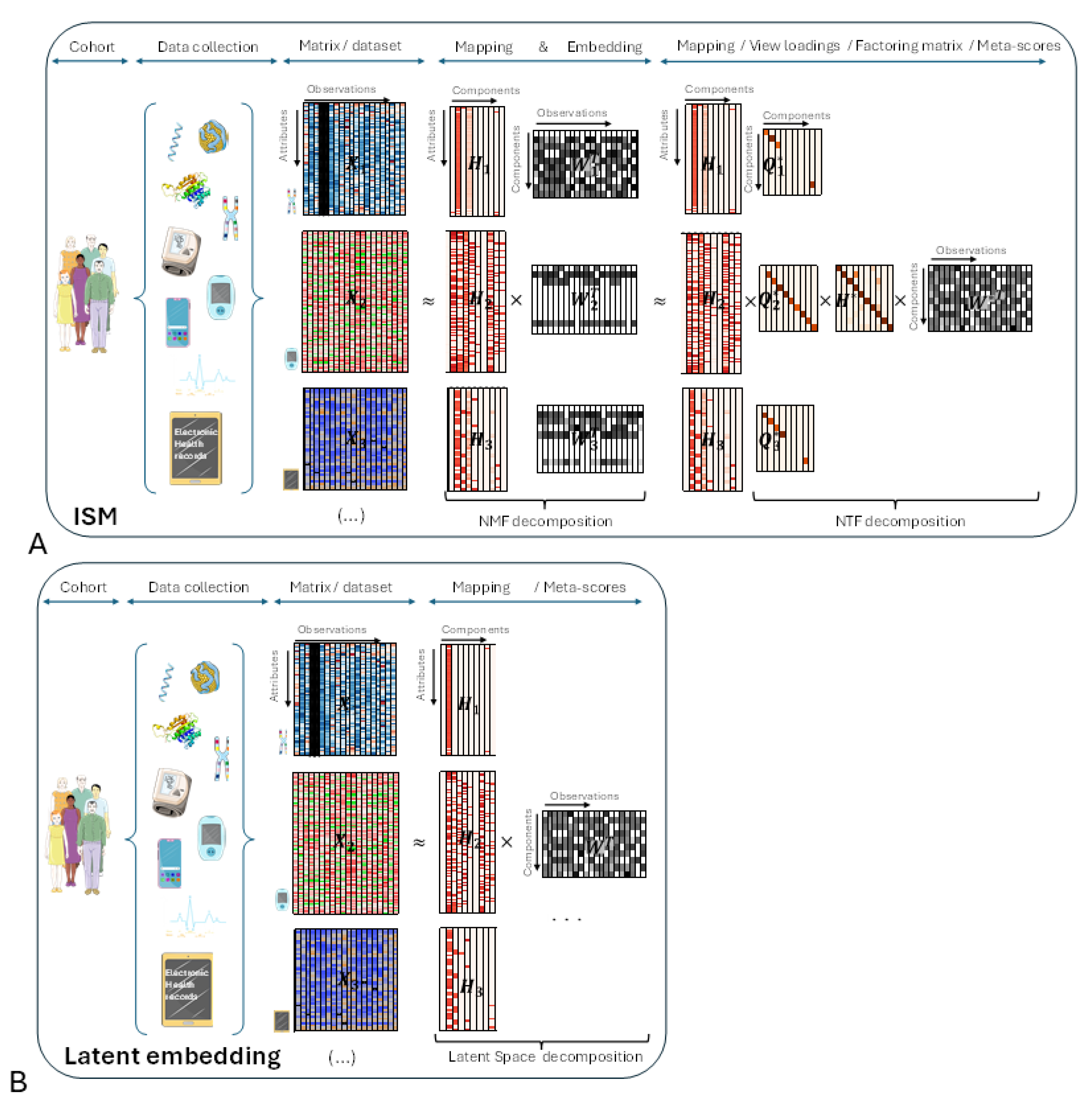
Figure 2.
Training of the ISM model.
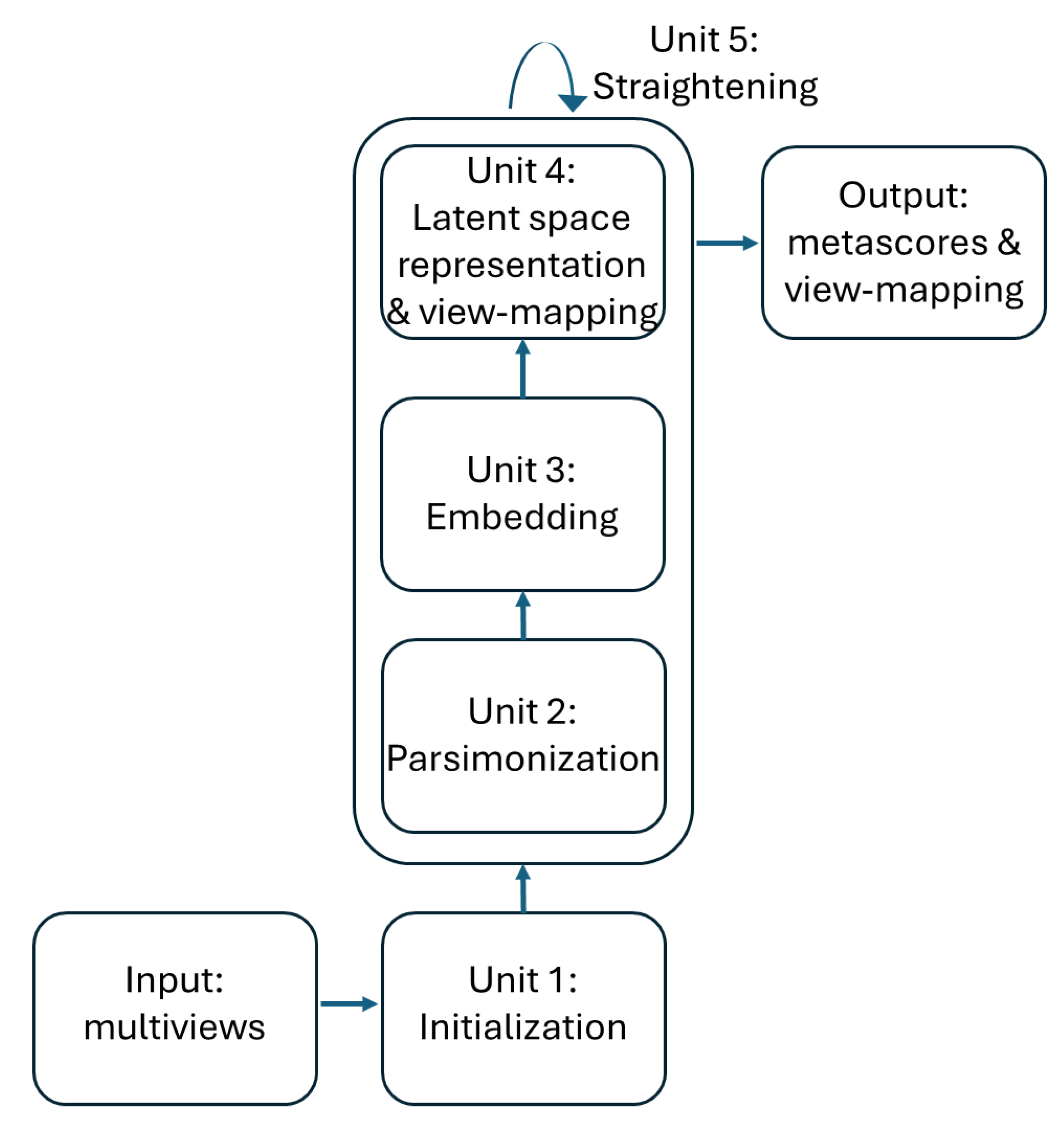
Figure 3.
UCI Digits Data: clustering of digit images along ISM, Multi-View Multi Dimensional Scaling (MVMDS), NMF and PCA components in 2D scatterplots of the MDS projection of transformed data. The left bottom view contains the MDS projection of the concatenated views.
Figure 3.
UCI Digits Data: clustering of digit images along ISM, Multi-View Multi Dimensional Scaling (MVMDS), NMF and PCA components in 2D scatterplots of the MDS projection of transformed data. The left bottom view contains the MDS projection of the concatenated views.
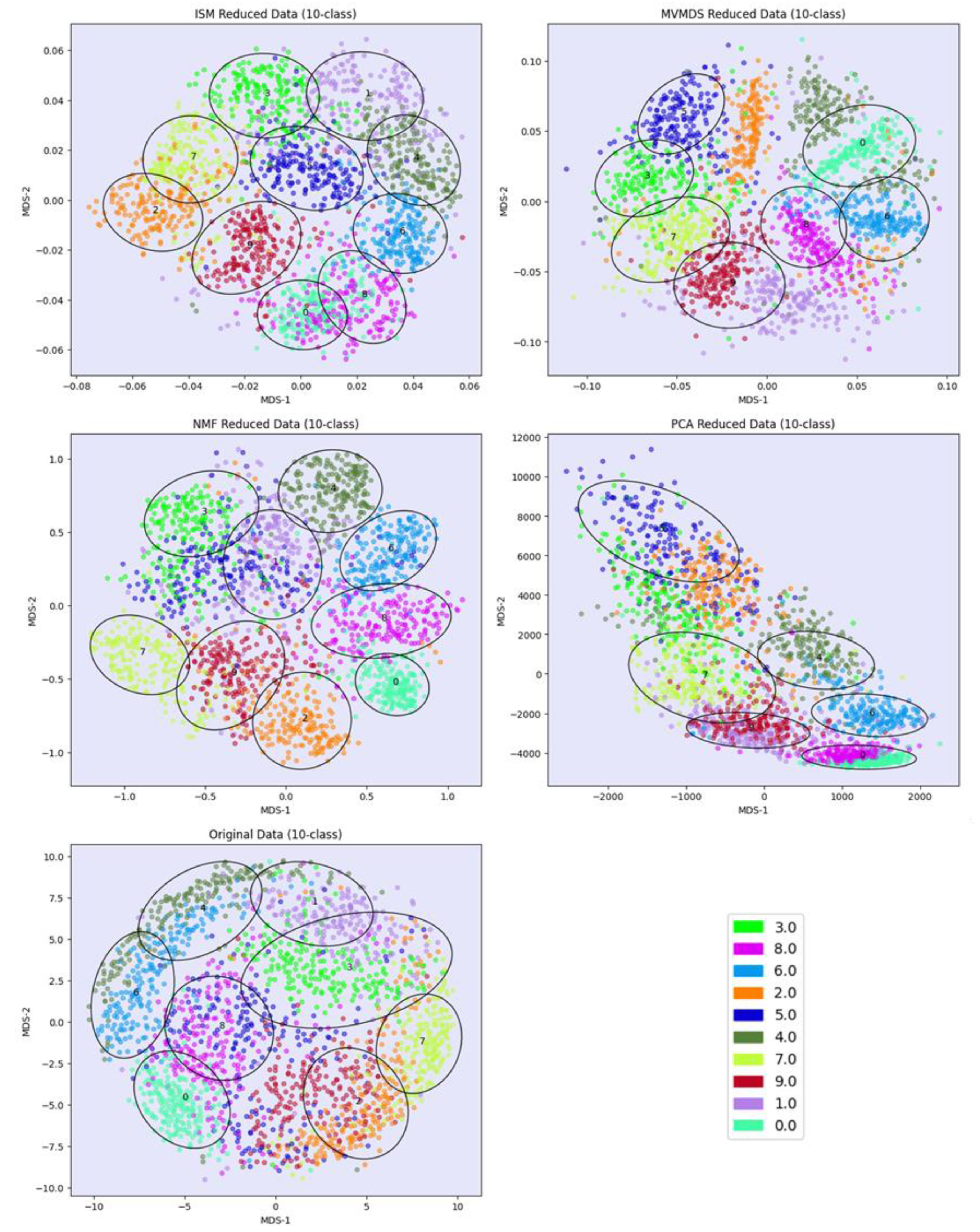
Figure 4.
UCI Digits Data: treemap of ISM view weights.
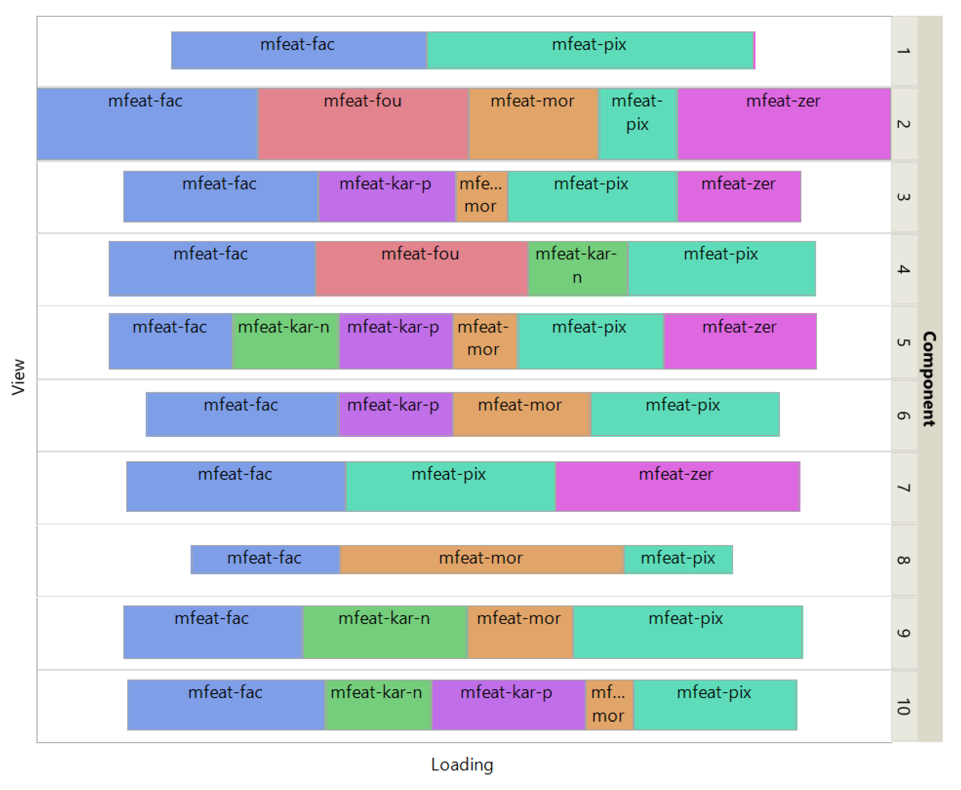
Figure 5.
Signature 915 Data: clustering of cell-type marker genes along ISM, MVMDS, NMF, NTF and PCA components in the 2D scatterplots of the MDS projection of the transformed data.
Figure 5.
Signature 915 Data: clustering of cell-type marker genes along ISM, MVMDS, NMF, NTF and PCA components in the 2D scatterplots of the MDS projection of the transformed data.
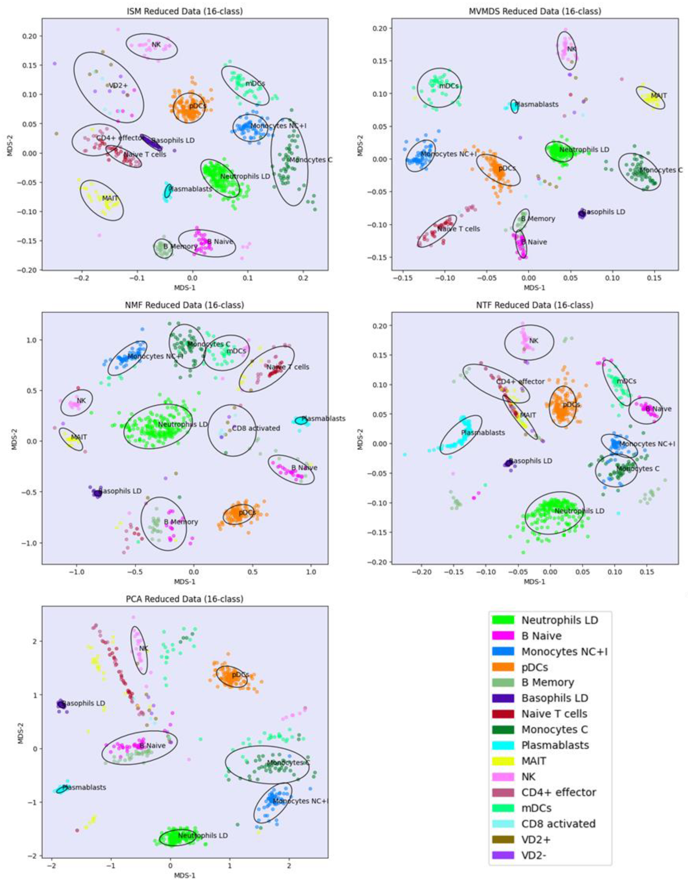
Figure 6.
Signature 915 Data: treemap of ISM view weights.
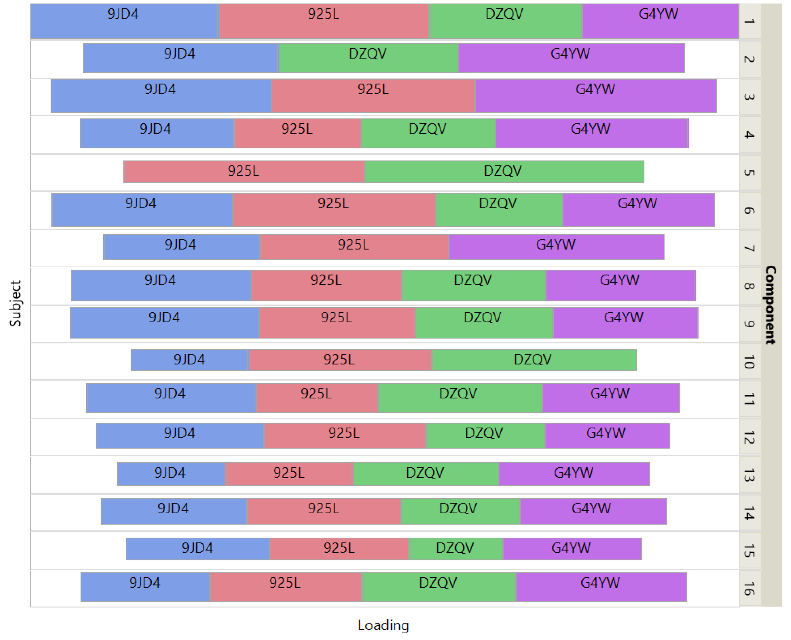
Figure 7.
Signature 915 Data: treemap of ISM loadings of the view-mapping matrix.
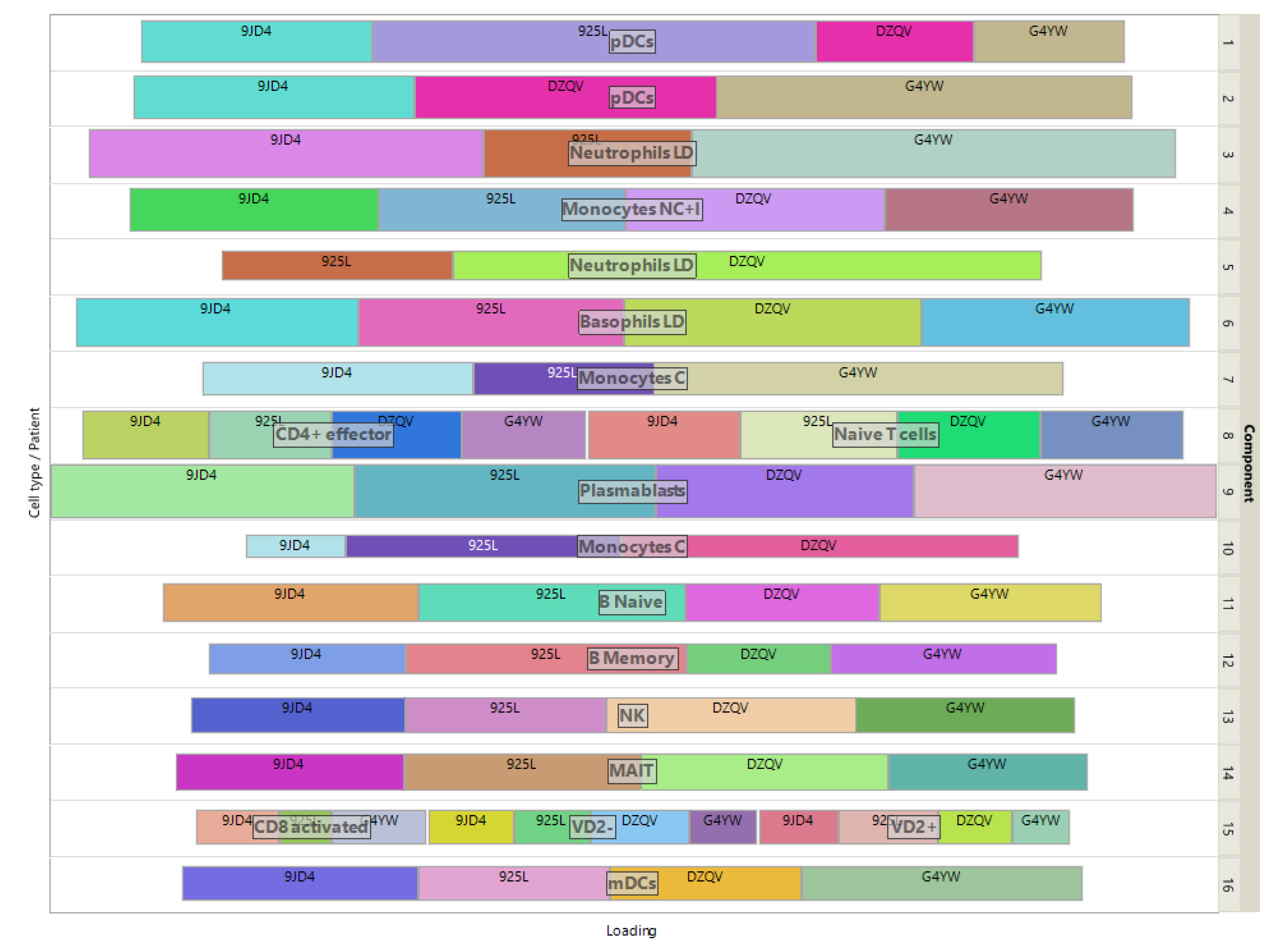

Table 1.
Number of found clusters and purity for 4 latent-space methods and using the concatenated data.
Table 1.
Number of found clusters and purity for 4 latent-space methods and using the concatenated data.
| Method | Number of clusters | Purity |
|---|---|---|
| ISM | 10 | 5.81 |
| MVMDS | 7 | 4.06 |
| NMF | 9 | 5.84 |
| PCA | 6 | 2.87 |
| Concatenated data | 8 | 3.34 |
Table 2.
Number of found classes and purity for 5 latent-space methods and using the concatenated data.
Table 2.
Number of found classes and purity for 5 latent-space methods and using the concatenated data.
| Method | Number of found classes | Purity |
|---|---|---|
| ISM | 14 | 11.46 |
| MVMDS | 12 | 11.19 |
| NMF | 13 | 8.78 |
| NTF | 11 | 8.39 |
| PCA | 8 | 6.68 |
| Concatenated data | 9 | 7.21 |
Table 3.
Relative error, number of found classes and purity as a function of the embedding dimension and rank (UCI digits data). In bold, the most performant combinations.
Table 3.
Relative error, number of found classes and purity as a function of the embedding dimension and rank (UCI digits data). In bold, the most performant combinations.
| Embedding dimension | Rank | Relative Error | Number of found classes | Purity |
|---|---|---|---|---|
| 8 | 10 | 0.84 | 7 | 2.96 |
| 9 | 10 | 0.52 | 10 | 5.81 |
| 10 | 10 | 0.72 | 5 | 2.07 |
| 11 | 10 | 1.2 | 8 | 4.73 |
| 12 | 10 | 0.91 | 7 | 3.22 |
| 9 | 12 | 0.6 | 10 | 6.24 |
| 9 | 11 | 0.62 | 9 | 4.15 |
| 9 | 10 | 0.52 | 10 | 5.81 |
| 9 | 9 | 0.52 | 8 | 3.58 |
| 9 | 8 | 0.7 | 8 | 3.5 |
Table 4.
Relative error, number of found classes and purity as a function of the embedding dimension and rank (Signature 915 data). In bold, the most performant combinations.
Table 4.
Relative error, number of found classes and purity as a function of the embedding dimension and rank (Signature 915 data). In bold, the most performant combinations.
| Embedding dimension | Rank | Relative Error | Number of found classes | Purity | |
|---|---|---|---|---|---|
| 14 | 16 | 0.36 | 10 | 8.77 | |
| 15 | 16 | 0.33 | 12 | 11.09 | |
| 16 | 16 | 0.34 | 14 | 11.46 | |
| 17 | 16 | 0.34 | 13 | 10.76 | |
| 18 | 16 | 0.38 | 13 | 11.92 | |
| 16 | 18 | 0.31 | 10 | 8.81 | |
| 16 | 17 | 0.32 | 14 | 12.12 | |
| 16 | 16 | 0.34 | 14 | 11.46 | |
| 16 | 15 | 0.34 | 14 | 11.66 | |
| 16 | 14 | 0.39 | 11 | 9.59 |
Disclaimer/Publisher’s Note: The statements, opinions and data contained in all publications are solely those of the individual author(s) and contributor(s) and not of MDPI and/or the editor(s). MDPI and/or the editor(s) disclaim responsibility for any injury to people or property resulting from any ideas, methods, instructions or products referred to in the content. |
© 2024 by the authors. Licensee MDPI, Basel, Switzerland. This article is an open access article distributed under the terms and conditions of the Creative Commons Attribution (CC BY) license (http://creativecommons.org/licenses/by/4.0/).
Copyright: This open access article is published under a Creative Commons CC BY 4.0 license, which permit the free download, distribution, and reuse, provided that the author and preprint are cited in any reuse.


