Leveraging the Sensitivity of Plants with Deep Learning to Recognize Human Emotions

Recent advances in artificial intelligence combined with behavioral sciences have led to the development of cutting-edge tools for recognizing human emotions based on text, video, audio, and physiological data. However, these data sources are expensive, intrusive, and regulated, unlike plants which have been shown to be sensitive to human steps and sounds. A methodology is proposed to use plants as human emotion detectors. Electrical signals from plants are tracked and labeled based on video data. Labeled data are then used for classification. MLP, biLSTM, MFCC-CNN, MFCC-ResNet, and additionally, Random Forests, 1-Dimensional CNN, and biLSTM without windowing models are set using a grid search algorithm with cross-validation. Finally, best-parameterized models are trained and used with the test set for classification. The performance of this methodology is measured with a case study with 54 participants, who were watching an emotionally charged video, as ground truth their facial emotions were simultaneously measured using face emotion analysis. The Random Forest model shows the best performance, particularly in recognizing high-arousal emotions, achieving an overall weighted accuracy of 55.2% and demonstrating high weighted recall in emotions such as fear 61.0% and happiness 60.4%. The MFCC-ResNet model offers decently balanced results, with Accuracy(MFCC-ResNet)=0.318 and Recall (MFCC-ResNet)=0.324. With the MFCC-ResNet model fear and anger are recognized with 75% and 50% recall respectively. Thus, using plants as an emotion recognition tool seems worth investigating, addressing both cost and privacy concerns.

Keywords:

Subject: Computer Science and Mathematics - Artificial Intelligence and Machine Learning

1. Introduction

Emotions are an integral part of the human being. They condition our actions and decisions [1]. There’s nothing more personal than an emotion, and yet, Ekman and Friesen [2] has demonstrated the universal nature of basic emotions, enabling everyone to recognize them, independently of their culture or education.

Human emotion recognition is a widely studied topic in human behavioral research. Different types of data such as video [3,4,5], speech [6,7], and text [8,9,10] are used for analysis. However, the high cost (in terms of acquisition, operation, and maintenance) as well as the privacy intrusiveness and regulations surrounding these types of data are an obstacle to the development of human emotion detection [11]. Unlike these sensors, which are difficult to accept, plants are part of people’s daily lives. In addition to their benefits for the quality of human life [12], it has been shown that plants can sense human steps [11] and sounds [13]. The question then arises if this ability of plants can be leveraged to detect human emotions?

This article proposes a methodology using plants as sensors to detect human emotions. This approach addresses the concerns and high costs of traditional emotion tracking methods and will pave the way for new research in human emotion detection and recognition.

The article is structured as follows. Section 2 will provide an overview of the research on human emotion detection as well as the use of plants as sensors. Then, Section 3 will present the material and methodology necessary to use plants as human emotion detectors. Section 4 will describe the results obtained by applying the proposed methodology to a real-world experiment. Limitations and directions for further research will be discussed in Section 5. Finally, Section 6 will conclude the article by recalling the contribution and limits of the proposed methodology as well as future research directions.

2. State of the art

Although both plants and emotions are an integral part of people’s daily lives, the use of the former to recognize the latter is unprecedented. In order to better understand the foundations supporting the development of a methodology enabling the use of plants as human emotion detectors, an overview of the research on emotion recognition (SubSection 2.1) and plant-based sensors (SubSection 2.2) is given in the following section.

2.1. Emotion recognition

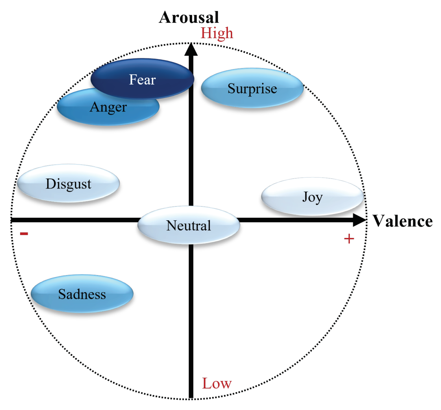
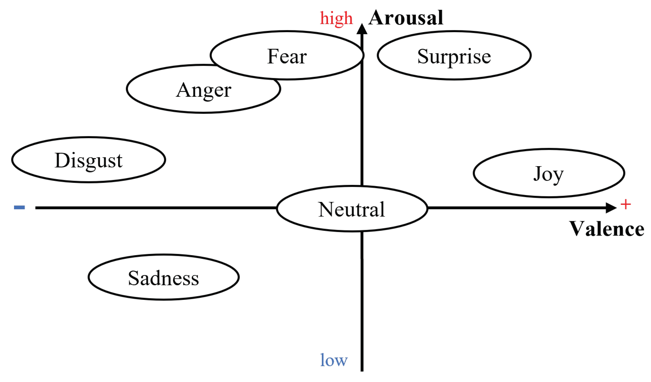
What could be more personal than an emotion? Emotions reflect an automatic, unconscious evaluation of a situation, based on past personal experience and human evolution [14]. Thus, emotions are, by definition, subjective and personal. Since each person has their own personal history, the same situation can provoke a wide variety of emotions of varying intensity in different people [15]. Despite the various psychological and philosophical debates on the rational (cognitive and intellectual) or irrational (emotional and social) nature of human beings [16], the power and omnipresence of emotions, as well as their influence on decision-making is widely accepted [1]. Emotions have a major influence on an individual’s reactions (choices and actions) and on the assessment of others’ behavior in a given situation [15]. The structure of emotional spaces is still up for debate [17]. Since Darwin [18], first introducing the notion of emotions, different approaches have been proposed. For Ekman [19], six basic emotions are present in all cultures recognizable by the same facial expressions. This supports the universalist theory of emotions to the detriment of the cultural hypothesis [2,14]. Thus, for Ekman [19], fear, anger, joy, surprise, disgust, and sadness are the primary colors of the chromatic palette of emotions. When the basic emotions are mixed, they form a vast variety of more complex emotions such as pride, excitement or amusement [14]. Others, such as Russell [20], model emotions on a continuum. The Valence-Arousal model describes a person’s emotional state according to the level of pleasantness (valence positive or negative) and arousal (arousal high or low) of the emotion felt [20]. These two models are not mutually exclusive. Indeed, the six basic emotions defined by [19], and the resulting complex emotions, can be placed on the continuum proposed by [20] as illustrated in Figure 1.

With the advancement of new technologies and the constant increase in computing power, those conceptualizations of human emotion form the basis of automatic emotion recognition (AER). Although the discrete conceptualization of emotions (such as Ekman [19]) resulting in a classification problem is cited frequently in the relevant literature [17], the continuum Valence-Arousal can also be used for regression purposes [4,5]. Regardless of the chosen framework, a wide range of data sources can be used to detect emotions.

Text analysis is one of the most widely used techniques, due to the abundance of opinions and emotions shared by individuals on social networks or e-commerce platforms [9,10]. Emotion detection from text can be handled by a keyword-based approach or, more rarely, a rule-based approach. However, the most commonly used approach is based on learning, since it offers the best performance to deal with the implicit expression of emotions (such as irony or sarcasm) [9,10]. Within this approach, we find machine learning tools (support vector machine (SVM), decision trees, random forest (RF), k-NN or Hidden Markov Model (HMM) [8]) and deep Learning tools (Convolutional Neural Network (CNN), Long-Short Term Memory (LSTM) and transformers) [9,10]. SVM, CNN, and LSTM are also commonly used for emotion detection using image analysis [3].

Image analysis is extremely relevant for emotion detection since two-thirds of the information transmitted by an individual is in the form of non-verbal elements, particularly through facial expressions [3]. The work of Ekman and Friesen [21] makes it possible to characterize the basic emotions described by Ekman [19] felt by an individual according to facial expressions. More recently, these hand crafted-attributes used in conventional methods have been replaced by training automated facial emotion recognition (FER) models such as Mühler [22] which automatically generate attributes for classification [3]. Although non-verbal information is omnipresent, speech remains the most natural and fastest method of communication for humans. Speech analysis is therefore an important element of AER.

Speech analysis uses the same classification tools as image or text analysis. These include machine learning methods such as SVM, HMM, or k-NN [6] but also deep learning approaches such as DNN, CNN, and LSTM [7]. One of the most important challenges faced in speech analysis is the extraction of attributes with significant emotional representativeness, regardless of the lexical content used. El Ayadi et al. [6] describes continuous, qualitative, spectral, and Teager-energy-operator (TEO)-based attributes as the four categories of attributes that can be extracted from speech analysis. Spectral attributes are used as a short-term representation of speech signals and Mel-frequency cepstral coefficients (MFCC) feature extraction is an important data-processing tool since those features hold promise for the representation of speech for multiclass classification [6]. Although many advances have been made in the use of text, images, and speech for emotion recognition, they are based on elements that can be consciously manipulated by individuals. Physiological data will limit that risk.

The expression of emotions generates physiological changes in individuals which are hard to fake [23]. Thus, data from physiological data such as brain activity (EEG), body temperature, heart rate signals (ECG), muscle activity (EMG), sweat levels or respiration levels can be used as "honest" input into emotion recognition models [23]. Once again, machine learning and deep learning tools such as SVM, k-NN, RF, CNN, LSTM and DNN are used in those contexts.

The influence of emotions on people’s choices and behavior makes AER an exciting field of study for many sectors such as robotics, marketing, education, health care [9,10] and also finance [8].

However, the high cost (in terms of acquisition, operation, and maintenance), as well as the privacy intrusions and regulatory restrictions of collecting these types of data (video, audio, text, EEG, etc.), are an obstacle to the development of automated human emotion detection systems [11].

2.2. Using plants as sensors

Unlike cameras, microphones, or EEG, plants are part of people’s daily lives. In addition to their benefits for the quality of human life [12], it has been shown that plants can be used as sensors that are able to monitor their environment [24]. More precisely, plants are sensitive to changes in luminous intensity, pressure, and temperature as well as changes in the electromagnetic or gravitational field [25]. They respond to these environmental changes by generating different types of electrical signals within and between cells [24]. The effects of environmental changes on plants can be rapidly observed thanks to the propagation speed of bioelectric signals, ranging from 0.05 cm/s to 40 m/s [25]. To detect electrical reactions in plants, electrodes can be placed on the plant [26] or directly inside the plant, in contact with the targeted cells [27]. The resulting signal corresponds to the difference in potential between the plant cells and the soil.

The use of electrical signals emanating from plants as sensors has been exploited in a limited number of works. Chatterjee et al. [28] uses electrical signals from tomato plants to recognize the chemicals to which the plants are exposed. Signals collected using internal electrodes placed in roots, stems and leaves are statistically processed and the extracted attributes are used as input to a linear discriminant analysis (LDA) classification model. The study classifies with an accuracy of approximately 70% the sodium chloride (NaCl), sulphuric acid (H2SO4), and ozone (O3) to which plants are exposed.

In addition to their ability to recognize chemicals, plants can also be useful for recognizing individuals and their moods (happy or sad) [11]. Oezkaya and Gloor [11] use external electrodes with the SpikerBox [29] to record electrostatic changes caused by a person’s gait. The signal generated by the plant is processed by MFCC and then classified using a random forest (RF) model. Using this method, one can recognize one individual among six others with an accuracy of 66%. It can also determine a person’s mood with an accuracy of 85%. Finally, Peter [13] showed that plants are also sensitive to sound. Using statistical modeling of plant signals combined with an MLP classifier, the three sounds used in the experiments were classified with an accuracy of 72%.

Thus, it has been shown that the external sensing capabilities of plants can be used for the development of sensors with a quality comparable to that of dedicated devices. With simple, inexpensive operations and no need to record personal data, plants appear to be an interesting data-acquisition tool that remains relatively unexploited. In the remainder of this paper we investigate the ability of plants to detect human emotions.

3. Method

Traditional sensors to capture human emotions are often perceived as intrusive, they are highly regulated and can be costly to acquire, operate, and maintain. On the other hand, plants are an integral part of our environment. In addition to their aesthetic aspect, it has been shown that plants are endowed with an astonishing capability for sensing their environment [11,13,28]. This study seeks to further this knowledge and proposes a methodology enabling the use of plants as human emotion detectors. To test this research hypothesis, a research method was developed and verified in an experiment.

3.1. Experimental setup

To develop a methodology to detect human emotions with a plant, an experiment was designed to simultaneously collect the emotions of an individual and the reactions of the plant-based sensor to the human [30]. The purpose of the experiment was to induce strong emotions in the participant and to record the responses obtained by the plant-based sensor. The experiment was structured into 5 steps:

1.: First, the participant’s consent was collected and the observer in charge of running the session answered any open questions.
2.: Then the observer quickly described to the participant the task that they would be asked to perform. The task was to watch a video sequence designed to elicit strong emotional responses from participants. The video sequence was created based on previous work by Gloor et al. [31] and is described in Table 1.
3.: The participant then sat in the experimental room and the sensors (plant and camera) were activated. Figure 2 is a photograph of the experimental set-up.

A screen displays the videos that elicit the participants’ emotional reactions (see Table 1). These reactions are filmed by a wide angle camera placed just below the screen. The camera is set up to obtain a zoomed image of the participant’s face. Finally a basil plant Ocimum basilicum, equipped with a sensor SpikerBox [29] is positioned in front of the participant.
4.: Then the observer started the video sequence and left the room to let the participant watch the video.
5.: Once the video sequence was finished, all sensors were deactivated and the data collected by the plant sensor and the camera was saved.

This protocol was repeated for each participant in the study. As participants watched those videos, their emotional reactions were recorded by the plant-based sensor and the camera. The individual files were then stored in two data bases named "plant signals" and "video".

3.2. Analysis

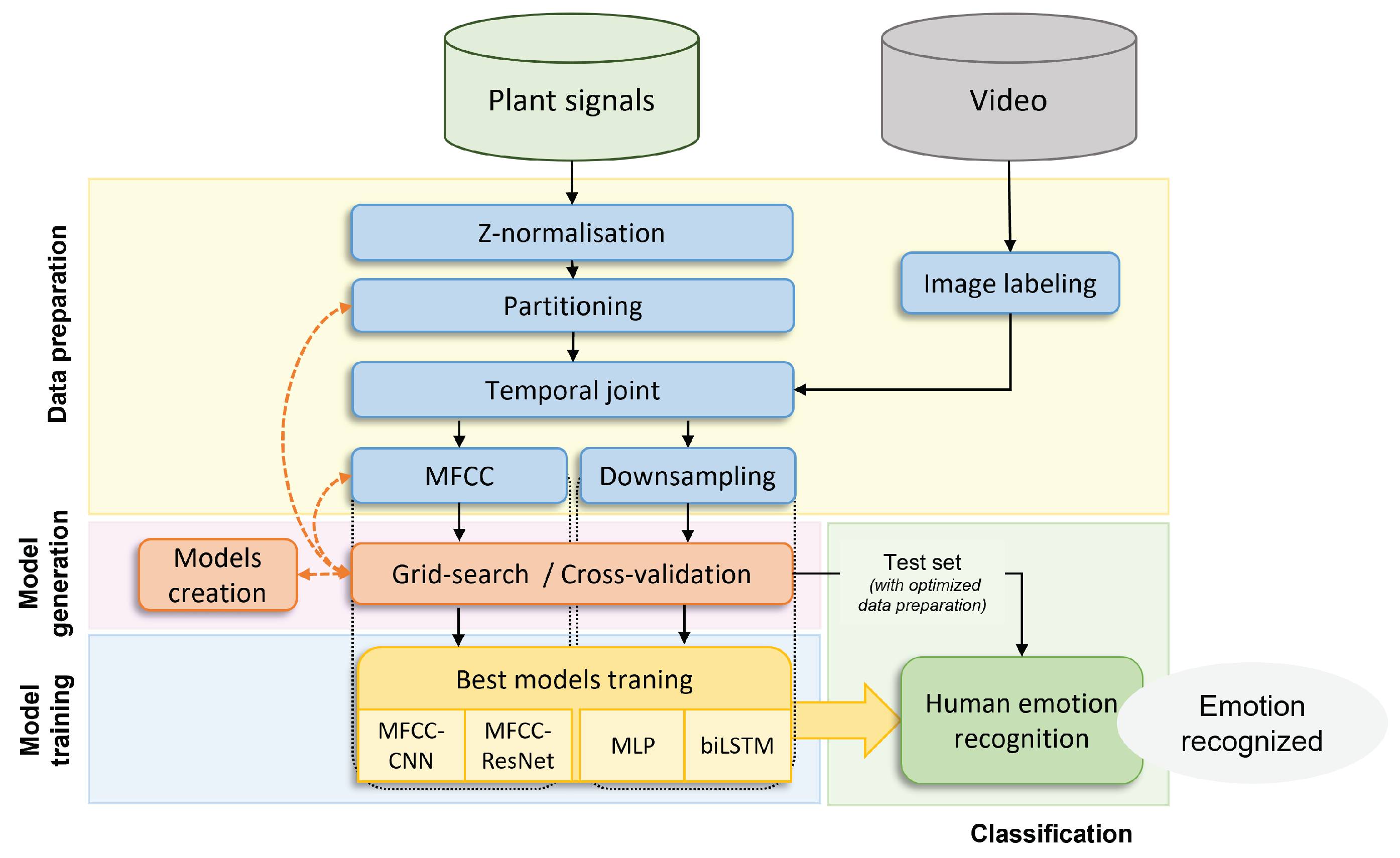
To analyze the data of plants as detectors of human emotions, the four-step algorithm illustrated in Figure 3 was used.

First, the data was preprocessed. The plant signals were cleaned and formatted so that the classification algorithms could use them. They were also labeled using video data, which computed the emotions felt by the participants during each second of the experiment from their facial expression. Once the plant signals were formatted and labeled, they were used in the subsequent classification model generation step.

In the classification model generation step, different deep-learning models were tried and parameterized using the cross-validation and Grid-Search algorithms. The Grid-Search algorithm used the cross-validation folders to find the best combination of hyperparameters for both model architecture and data preparation.The best parametrization for each of the models was saved and used in the model training step.

In the model training step, training and validation sets were once again used to further train the selected models. The trained models were finally tested with the test set. The goal was for the plant sensor to exclusively predict the emotion of the viewer.

Each step of the methodology is detailed below.

3.3. Data preparation

Data preparation is a necessary step to transform raw data into data that can be used by artificial intelligence algorithms. Although both data sources must be pre-processed, the signals from the plant sensor undergo more significant transformations. In our research, we implemented two distinct methodologies for data preprocessing, each yielding divergent outcomes. The initial method, henceforth referred to as "MFCC Extraction," involves segmenting the electrical signal into 20-second intervals, followed by the extraction of Mel Frequency Cepstral Coefficients (MFCC) from these segments. The second method, which we designate as "Raw Signal Analysis," entails isolating 1-second fragments from the raw electrical signal. These fragments directly correspond to facial emotions detected over a 1-second duration. This approach focuses on analyzing the amplitude variations within the signal. The methodologies are described in detail in the subsequent sections.

3.3.1. Initial data preparation approach - MFCC extraction with windowing

First, each signal must be treated in order to limit the effect of the experimental conditions on the signal analysis. Indeed, although the experimental conditions are controlled, interferences due to the environment or the position of the sensors on the plant can alter the signal. These conditions are considered constant throughout the same experimental session. The signals are normalized using a z-normalization on a per-file basis.

Then the signal is partitioned in order to transform it into a set of shorter windows. Each window represents a portion of the normalized signal whose length is determined by the hyperparameter window expressed in seconds. Another hyperparameter named hop allows one to choose the number of seconds between the beginning of two successive windows. This specificity allows the succession of overlapping time windows if the hop value is smaller than the window window size. This is the principle of the sliding window used in time series processing. Those hyperparameters are tuned using the cross-validation and Grid-search algorithm presented in the following step of the methodology.

In order to classify the responses of the plant according to the emotions felt by the participants, it is important to collect the real emotion felt by them. Image analysis for emotion detection has been widely studied and recognized by the scientific community (See Section 2.1). Thus, the emotions recognized in the images extracted from the videos are used as ground truth in order to label the signals obtained by the plant-based sensor. During the image labeling, each second of the video results in the extraction of an image. Those images then are used as input to the well-known emotion detection model face-api.js [22] to obtain the emotion felt by the participant during the one-second window considered.

A temporal join is then used to associate the labels obtained from the video input with the processed signals obtained from the plant sensor. The plant data window labels are assigned based on the label at the end of the data window. Furthermore, data points where the label proposed by face-api.js does not match the expected emotion specified in the column Expected emotion of Table 1 are excluded. The emotions to be detected are stored in an emotion list containing

n b_{e m o t i o n}

different emotions.

Finally, two independent data sets are created from the short plant signals.

The first dataset consists of the downsampled short-plant signals. Since the plant sensor has a high sampling rate (10kHz), a downsampling of the signals is required before feeding them into the different training models. Downsampling reduces the complexity of the signal while retaining the relevant information [11]. Its rate is a hyperparameter called downsampling rate whose value is determined by trial and error.
The second dataset consists of the computation of MFCC features from each window. The result is a 2D matrix of shape [time steps, number of MFCCs] that can be processed by various deep learning algorithms such as LSTM or CNN.

Obtaining these two data sets concludes the first step of the methodology, the data processing. The classification models as well as the optimization of the hyperparameters can be initiated in the second step of the methodology, the model generation.

3.3.2. Alternative data preparation approach - raw electrical signal analysis

In contrast to the previous approach, the alternative data preparation method focuses on analyzing the raw electrical signals from the plant sensor without downsampling and windowing. This approach aims to explore the full complexity and granularity of the data, potentially revealing subtle nuances in the signals that are associated with different emotional responses in participants.

The electrical signals are captured from a SpikerBox [29] attached to a plant in the same environment as participants viewing emotional videos. Each participant’s electrical signal data, represented as an array, consists of 6,900,000 samples, reflecting the sampling rate of the sensor (10,000 Hz) and the total length of the watched videos (690 seconds). The ground truth for emotions is derived from video recordings, labeled with timestamps and corresponding emotions.

The raw electrical signals are processed without downsampling to preserve the original signal fidelity. The signal for each participant is segmented into 1-second intervals, corresponding to the timestamps of the emotion data. This segmentation results in 690 segments per participant, each containing 10,000 samples. Each signal segment is normalized using z-normalization to reduce the impact of variations in signal amplitude and to facilitate comparability across different participants. Instead of downsampling or computing MFCC features, this approach focuses on analyzing the raw, normalized signal data. This decision is based on the hypothesis that the high-resolution data might contain intricate patterns associated with different emotional states.

The labeled emotions from the video data are used to tag each corresponding signal segment. The process involves aligning the timestamps from the emotion data with the signal segments, ensuring that each segment is labeled with the corresponding emotional state of the participant at that specific second. The normalized signal segments and their associated emotion labels are integrated into a cohesive dataset. This dataset forms the basis for the subsequent modeling and analysis, wherein the relationship between the raw electrical signals and the participants’ emotions had been explored.

The final dataset comprises two main components: the normalized electrical signal segments and their corresponding emotion labels. This dataset is ready for the next phase of the study, which involves the development and training of models to classify the signals based on the emotional states of the participants.

3.4. Models generation

The generation of classification models allows for the definition of their architecture and also their parameterization. Many hyperparameters influence the performance of the studied models which is why it is important to choose them carefully.

The creation of the models aims at defining the general architecture of the different models considered for the detection of human emotions from plant signals. This task corresponds to a multiclass classification of time series. As neural networks are known to perform well on those tasks (see SubSection 2.1), three different types of architectures are considered. Table 2 summarizes the key elements of the architecture of each model. All models were producing an output of a vector of size

[1, n b_{e m o t i o n}]

representing the probability of occurrence of each detected emotions present in the emotions list.

A fully connected Multi-layer Perceptron neural network (MLP) is used as a baseline, while an LSTM-based model (biLSTM) and CNN-based models (MFCC-CNN and MFCC-ResNet) are used to process downsampled signals and MFCC features, respectively. The ResNet is a deeper convolutional network proposed by He et al. [32] and trained on ImageNet [33]. The model MFCC-ResNet uses the neural network ResNet to process the MFCC data extracted during the data preparation phase. In this work, the architecture of the neural network ResNet was slightly modified to fit the emotion detection task. Indeed, the last layer of every model is expected to be a dense layer activated by the SoftMax activation function and containing

n b_{e m o t i o n}

neurons each representing one of the detected emotions present in the

E m o t i o n s

list. Additionally, for the raw, unwindowed plant electrical data, a Random Forest model is employed, taking advantage of its ability to handle diverse datasets efficiently. It operates using a large ensemble of decision trees, configured with parameters like the number of trees and maximum depth, to ensure a balance in managing complex classification tasks. A 1-Dimensional CNN (1D CNN) is also utilized for the data, particularly suited for analyzing time-series data such as raw plant electrical signals. This model consists of a sequence of convolutional and pooling layers, followed by dense layers with a ’softmax’ activation function in the output layer for class probability estimation. Lastly, another variant of the LSTM model, the biLSTM, is applied to capture long-term dependencies in the time-series data. This model’s architecture features bidirectional LSTM layers followed by dense layers, fine-tuned to optimize performance for emotion detection tasks. All models share the common trait of outputting a probability vector, indicating the likelihood of each emotion detected in the dataset. The output vector of all models is then a probability vector of size [1,

n b_{e m o t i o n}

Each of those models has hyperparameters that are important to optimize to ensure their best performance. Table 3 presents the specific values associated with each of the models’ hyperparameters that should be tested during the grid-search.

In addition to the hyperparameters specific to each model, general hyperparameters related to data preparation or model training must also be taken into account. Table 3 summarizes all these hyperparameters and defines the ranges of values to be tested during the optimization of hyperparameters by grid-search.

In all models considered, the optimization of the hyperparameters window and hop used in the partitioning task during the data preparation is needed. This is also the case for the learning rate and for balancing hyperparameters. The learning rate is used for the training of each model while the balancing hyperparameter is used to handle the unbalanced dataset. When the value balance is chosen, rare classes are oversampled while the majority classes are undersampled. In the case where the value weights is chosen, the weight of each class is incorporated into the loss function so that all classes have the same impact on this loss. Finally, if the value none is chosen, nothing is done to compensate for the data unbalancing.

The other hyperparameters are model specific. In the MLP model, the number of dense layers (dense layers), the number of neurons per layer (dense units), as well as the dropout rate (dropout rate), are hyperparameters inherent to the model. Similarly in the biLSTM model, the number of LSTM layers (LSTM Layers), the number of neurons per layer (LSTM units), and the dropout rate (dropout rate), are hyperparameters to optimize. In the MFCC-CNN model, the dropout rate, the number of convolutional layers (conv layers), as well as the output dimensionality (conv filter) and the size of the 2D convolution window (conv kernel size) are hyperparameters inherent to the model. Finally, In the MFCC-ResNet model, only two hyperparameters are model specific. The pretrained hyperparameter determines if the weights from the ImageNet training are used, while the number of MFCCs determines the number of MFCCs features extracted during the data preparation step. In the case of the Random Forest model, key hyperparameters include the number of trees in the forest (n_estimators), the maximum depth of the trees (max_depth), and the class weights (class_weight). For the 1D CNN model, important hyperparameters comprise the number of filters (filters), the kernel size (kernel_size) in the convolutional layers, the pool size (pool_size) in the pooling layers, and the number of neurons in the dense layers (dense units). The model is also characterized by its learning rate (learning_rate) and loss function (loss). Lastly, in the biLSTM model, critical hyperparameters include the number of LSTM layers (LSTM Layers), the number of units in each LSTM layer (LSTM units), and the learning rate (learning_rate) of the optimizer. These hyperparameters are crucial for fine-tuning the models’ performance in emotion detection tasks.

The combinations of each value presented in Table 3 are tested by training each classification model independently over a predetermined number of epochs.

3.5. Models training

To identify the best parameters for each model, a grid search of configuration is used with cross-validation. A five-fold cross-validation leads to a training, validation, and test split of 60%, 20% and 20% of the data.

Since the output of all presented models is a probability vector obtained from the SoftMax activation function, the standard associated loss function called categorical cross-Entropy (CE) is used for training [34]. As explained by Qin et al. [34], the measurement of the cross entropy between the true label y and the label ŷ resulting from the SoftMax activation function allows adjusting the model parameters by backpropagation. The stochastic gradient descent method known as the Adam optimizer [35], is used to train the models on the training data, grouped by batch size 64. Overfitting of the model is monitored using the validation set.

To measure the performance of the models during training, two metrics are used. The overall accuracy presented in equation 1 measures the rate of correct prediction of the model. The average recall per class presented in equation 2 measures the sensibility of the model. In other words, it measures the ability of the model to find a good positive class.

O v e r a l l A c c u r a c y = \frac{T P + T N}{T P + F P + T N + F N}

(1)

A v e r a g e R e c a l l p e r C l a s s = \frac{1}{n b_{c l a s s}} \sum_{\forall c l a s s} R e c a l l_{c l a s s} = \frac{1}{n b_{c l a s s}} \sum_{\forall c l a s s} {(\frac{T P}{T P + F N})}_{c l a s s}

(2)

\begin{matrix} W h e r e : \\ T P = T r u e P o s i t i v e \\ F P = F a l s e P o s i t i v e \\ T N = T r u e N e g a t i v e \\ F N = F a l s e N e g a t i v e \end{matrix}

During the grid search, each configuration is tested with the train and validation sets of different folds. Thus the whole dataset is found at least once in the test. The models are trained on a limited number of epochs. Using the EarlyStopping function, the training can be stopped if the loss on the validation set does not improve after a predetermined number of epochs called patience. The performance of each configuration is the average of the metrics (overall accuracy and recall) obtained for each fold.

Once this first training is done, the configuration having obtained the best score for each model is kept and will be used for the final training.

The final training is exactly the same as the one used during the grid search with the difference that the number of training periods is higher.

These can now be used in the last step, classification.

3.6. Classification

The classification step aims at feeding the trained models with new data never observed before (test set) in order to detect the emotion associated with the input signal. As was explained in subSection 3.4, the vector obtained in the output of the model is a vector of size

[1, n b_{e m o t i o n}]

representing the probability of each of the detected emotions according to the input signal used. The emotion recognized by the model from the input signal corresponds to the class associated with the highest probability in the resulting output vector of the model. The classification performance of the models is evaluated in the case study presented below (Section 4).

4. Results

The methodology described in Section 3.1 was tested in an experiment with 71 participants to obtain data suitable for analysis.

4.1. Data collection

Video data and plant signals were collected during two sets of experiments performed in a controlled environment. The experiments were performed in accordance with the MIT Committee on the Use of Humans as Experimental Subjects (COUHES) guidelines.

In the first experiment, 40 individuals participated in the data collection as described in Section 3.1. Due to some malfunctions of the plant sensor (no signal recorded) during the experiment, 12 data points had to be removed from the data set leading to 28 data points.

The second experiment was conducted with 31 individuals. As with the first experiment, an analysis of the quality of the data collected identified 5 incomplete data points, leading to 26 data points as input for analysis.

The case study therefore focusses on the analysis of 54 data points using the methodology presented in SubSection 3.2.

4.2. Analysis

The data was analyzed using Python 3.8 and available libraries such as keras [36], scipy [37], scikit-learn [38] and Numpy [39]. The 54 data points of video data and plant signals were used as input. Subsequently normalization, partitioning, labeling as well as the downsampling and MFCCs extraction were executed. The dowsampling hyperparameter was empirically set to 500Hz. The video data was transformed into images with a frequency of 1Hz. These images were labeled using face-api.js [22]. The following emotions were computed:

A n g e r, D i s g u s t, F e a r, H a p p i n e s s, N e u t r a l, S a d n e s s, S u r p r i s e

The number of detectable emotions thus was

n b_{e m o t i o n} = 7

which is used for generating the models as described in Table 2.

The approach described above applies to the first four models in our study, where windowing and downsampling techniques were utilized. In contrast, for the last three models (Random Forest, 1D CNN, and biLSTM), a different preprocessing strategy was employed. These models did not utilize downsampling due to their distinct handling of the raw data. Furthermore, during the analysis, it was observed that the classes of emotions were significantly unbalanced when no windowing preprocessing was done. Specifically, a large majority of instances were being classified as Neutral, leading to skewed results.

To address this imbalance and enhance the performance of the last three models, the Neutral emotion was excluded from analysis. This adjustment resulted in a more balanced distribution of emotion classes and improved the models’ ability to distinguish between the remaining emotions. Consequently, for the Random Forest, 1D CNN, and biLSTM models, the set of emotions considered was reduced to six, namely Anger, Disgust, Fear, Happiness, Sadness, and Surprise. Therefore, in these cases, the number of detectable emotions was

n b_{e m o t i o n} = 6

. This modification was crucial for ensuring the effectiveness and accuracy of these models in emotion detection tasks, as outlined in Table 2.

To optimize the other hyperparameters, grid search was performed on the MIT SuperCloud high-performance compute cluster [40] using its GPU compute nodes with two Intel Xeon Gold 6248 20-core processors, 384GB RAM and two Nvidia Volta V100 GPUs with 32GB VRAM each. A maximum of 50 epochs was used for grid search. Table 4 synthesized the optimized parameters obtained by the grid-search algorithm for each model.

Once the hyperparameters were defined, model training was undertaken on the same MIT SuperCloud high-performance computing cluster as for the grid research. Final training was carried out over a maximum of 1000 epochs. The test set was then used to compute the overall accuracy (equation 1) and average recall per class (equation 2). In this study the number of classes was either

n b_{c l a s s} = 6

n b_{c l a s s} = 7

since there are

n b_{e m o t i o n} = 6

n b_{e m o t i o n} = 7

emotions.

4.3. Evaluation

The results obtained for each of the models are presented in Table 5. Since five-split cross-validation was used, the values presented in Table 5 correspond to the average from the five splits.

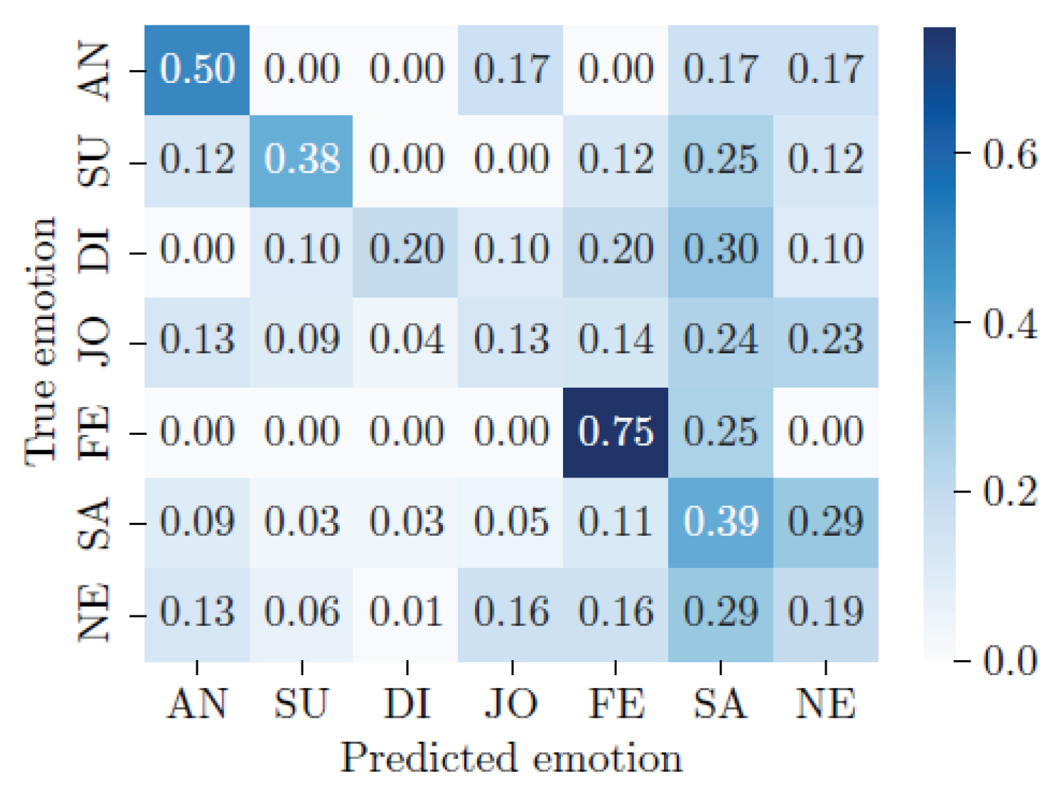
According to the results shown in Table 5, model MLP gives the best accuracy (

A c c u r a c y_{M L P} = 0.399

) but also the worst recall (

R e c a l l_{M L P} = 0.220

). This is often a sign of an overfitting on the majority class. This behavior can also be observed for the model MFCC-CNN (

A c c u r a c y_{M F C C - C N N} = 0.377

and

R e c a l l_{M F C C - C N N} = 0.275

). In the opposite case, the model biLSTM proposes a low

A c c u r a c y_{b i L S T M} = 0.260

but a relatively high

R e c a l l_{b i L S T M} = 0.351

. Finally, the model MFCC-ResNet proposes the best balance between accuracy and recall with respectively

A c c u r a c y_{M F C C - R e s N e t} = 0.318

and

R e c a l l_{M F C C - R e s N e t} = 0.324

. See Figure 4.

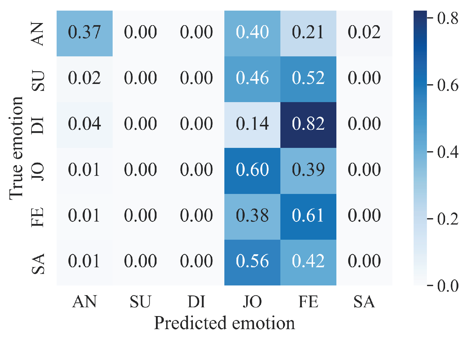
In contrast, the models utilizing "the raw data no windowing" preprocessing approach show different performance characteristics. The RF no windowing model achieved the highest accuracy (

W e i g h t e d A c c u r a c y_{R F n o w i n d o w i n g} = 0.552

) and recall (

W e i g h t e d R e c a l l_{R F n o w i n d o w i n g} = 0.552

) among all models, indicating a strong overall performance. The 1D CNN no windowing model also showed promising results with an accuracy of

A c c u r a c y_{1 D C N N n o w i n d o w i n g} = 0.461

and a recall of

R e c a l l_{1 D C N N n o w i n d o w i n g} = 0.514

, suggesting a good balance in its ability to correctly classify emotions. Lastly, the biLSTM no windowing model exhibited an accuracy of

A c c u r a c y_{b i L S T M n o w i n d o w i n g} = 0.448

and a recall of

R e c a l l_{b i L S T M n o w i n d o w i n g} = 0.380

, which reflects its competent performance though slightly lagging behind the RF and 1D CNN models in this specific setup. See Figure 5.

The confusion matrix resulting from the MFCC-ResNet model shows the model’s strong potential for detecting fear and anger, with 75% and 50% correctly predicted emotions for these two classes. Sadness is correctly detected in 39% of cases but can be mistaken for a neutral emotion or fear in 29% and 11% of cases respectively. Neutral, happiness, and disgust are difficult to predict for the model. The model’s performance for these classes is below 20% .

In comparison, the RF no windowing model shows a varied performance across different emotions. For anger (AN), it has a recall of 0.373, precision of 0.721, and an F1 Score of 0.492. The model is unable to effectively detect surprise (SU), disgust (DI), and sadness (SA), with recall, precision, and F1 Score all being 0.000 for these emotions. Happiness (JO) and fear (FE) are better detected, with the model achieving a recall of 0.604 and 0.610, precision of 0.556 and 0.540, and F1 Scores of 0.579 and 0.573, respectively. This indicates a stronger ability of the model to recognize emotions such as happiness and fear, while struggling significantly with surprise, disgust, and sadness.

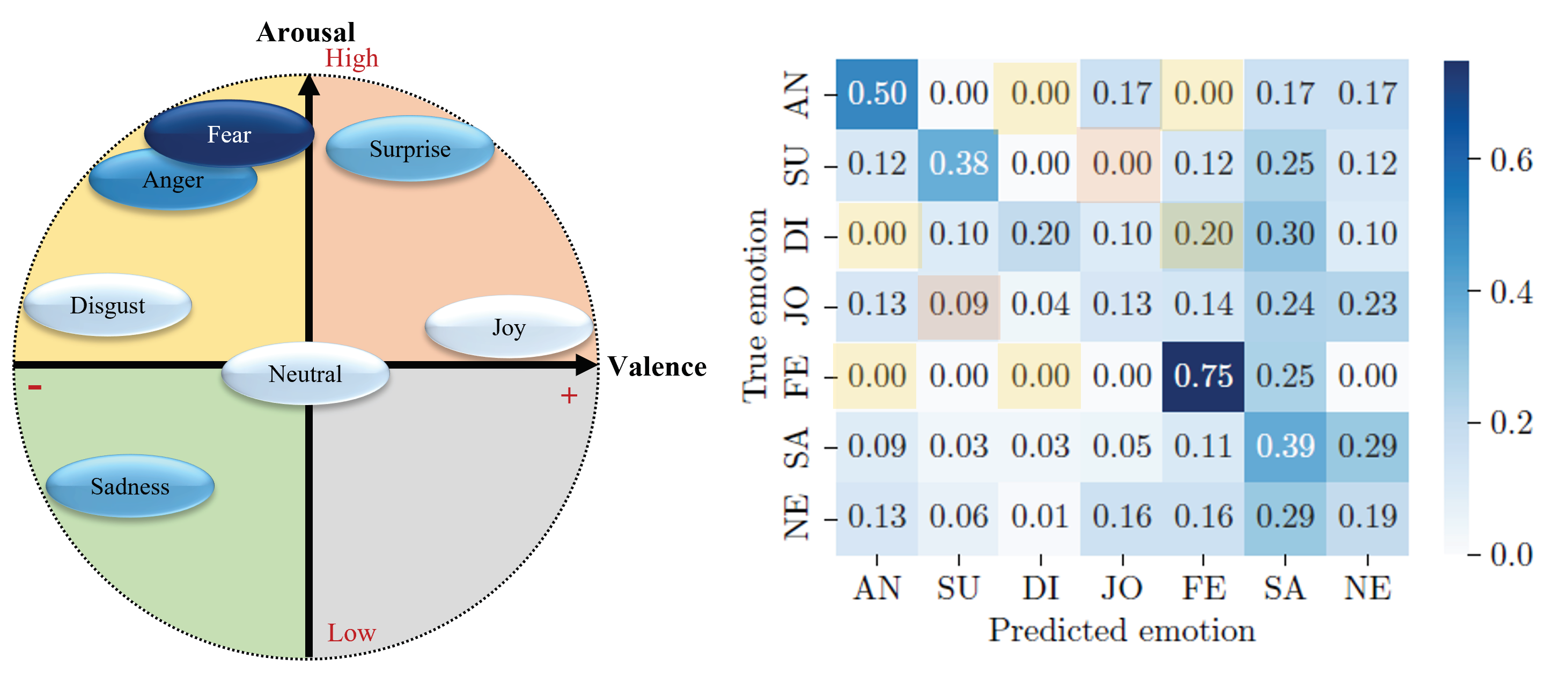
These results can be explained using Figure 6, with the valence-arousal emotional model from Russell [20] and the basic emotions of Ekman [19] presented in subSection 2.1.

As we can see on Figure 6, emotions with a high intensity of arousal, whether high or low, are relatively well predicted by the MFCC-ResNet model. Fear and anger are two emotions with a high arousal value and a negative valence. These two emotions are recognized best by the model, with 75% and 50% correct classifications. For the RF no windowing model, anger shows a moderate performance with a recall of 0.373 and an F1 Score of 0.492, while fear is better recognized with a recall of 0.610 and an F1 Score of 0.573.

Sadness has a relatively low arousal value and negative valence. The MFCC-ResNet model’s performance for classifying this emotion is equivalent to that for detecting the emotion of surprise, which has high arousal but positive valence. The rate of correct detection of the two emotions, symmetrical to the neutral emotion in the valence-arousal conceptualization of emotions, is equivalent to around 38%. Both emotions are poorly predicted by the RF no windowing model, with recall, precision, and F1 Scores all being 0.000 for sadness and surprise.

Finally, emotions with a medium level of arousal such as joy, disgust, and neutral emotion are difficult to classify by the MFCC-ResNet model, with a correct classification rate of no more than 20%. However, joy shows a relatively better performance in the RF no windowing model compared to disgust, with a recall of 0.604 and an F1 Score of 0.579.

Note that the accuracy for the MFCC-ResNet model is unweighted, which makes sense because the underrepresented categories have been oversampled during training to get a balanced distribution, as the original data distribution was as follows: anger: N=6, surprise: N=8, disgust: N=10, joy: N=95, fear: N=4, sadness: N=149, neutral: N=194. For the RF no windowing model the unbalanced data was directly used for the model, which led to higher weighted accuracy than for the MFCC-ResNet model. The N in this case is for fear: 141, joy: 4927, surprise: 390, anger: 588, sadness: 4676, and disgusted: 230.

Using the confusion matrix associated with the valence-arousal model of emotions also enables the analysis of the distribution of the model’s classification errors. Indeed, if the different emotions are grouped according to the quadrant to which they belong, as shown in Figure 7, one can see that the models rarely make classification errors within a single quadrant, but rather tend to decipher an emotion as belonging to another quadrant of the valence-arousal model.

The first frame, shown in orange in Figure 7, corresponds to emotions with positive valence and high arousal, i.e. surprise and joy. When surprise is detected, it is never confused with joy. Conversely, when joy is detected by the MFCC-ResNet model, it is confused with surprise in 9% of cases. Surprise is the second least confused with joy after disgust (4% confusion).

The MFCC-ResNet model’s ability to distinguish between emotions within the same quadrant is all the more apparent when the model’s second quadrant is studied. Since the frame represents a negative valence and a high arousal level, shown in yellow in Figure 7, no inter-class confusion is found, with the exception of the model’s classification of disgust as fear.

5. Discussion

Based on the results introduced above, the use of plants as sensors for emotion recognition deserves further investigating. The best model (MFCC-ResNet) shows an overall accuracy of nearly 32% and an average recall per class of 32.4%. The model is particularly good in recognizing emotions with high-arousal levels and negative valence with 75% and 50% of accuracy for the fear and the anger classes.

Furthermore, the RF no windowing model demonstrates even more promising results in this context. This model achieved an overall accuracy of 55.2% and displayed significant strengths in recognizing certain emotions. For instance, it had a high recall of 61.0% for fear, 60.4% for happiness, and 37.3% for anger, indicating its effectiveness in identifying these high-arousal, negative valence emotions. However, it is important to note that the model struggled with emotions like surprise, disgust, and sadness, as indicated by a recall and precision of 0.000 for these classes. This variation in performance across different emotions highlights the complexity of emotion recognition using plant signals and underscores the potential of further refining these models to improve their accuracy and recall across a broader spectrum of emotions.

This phenomenon might be explained by the type of sensor used to collect signals from the plant and the physiological responses associated with emotions. As described in Section 2.2, the SpikerBox sensor measures the potential difference between the plant and the soil. According to Rooney et al. [41], emotional arousal increases skin conductivity. Thus, the study of plants’ ability to detect variations in emotional arousal based on the electrical activity of individuals’ skin could be explored in future research.

Another hypothesis would explain the model’s performance by the physical reactions triggered by the respective emotions. Emotions such as fear, anger or surprise lead to more body movements than emotions such as disgust or joy. The latter emotions result in small movements, often facial expressions, which only marginally influence the environment surrounding the plant. Thus the strength of the physical reactions triggered by an emotion could explain the model’s recognition performance.

The fact that the emotion of sadness is also overused for the classification of other emotions also raises the question of the uniqueness of sadness. Although considered a basic emotion by [19], Shirai and Suzuki [42] argue that sadness is not unique and is more complex. "The exact nature of sadness is still quite vague in comparison to other emotions" [42], this vagueness could be one of the explanations for the lack of precision observed in the classification of sadness. Since signal labeling is based on the recognition of emotions on images (see Section 3.3.2), a poor definition of the emotion of sadness can lead to poor signal labeling, resulting in model confusion for this class.

Nevertheless, these results also demonstrate that deep learning tools typically used for multiple classification tasks such as emotion recognition can also be used to process signals from plants. As mentioned by He et al. [32], the depth of the CNN network does have a positive impact on model performance (

R e c a l l_{M F C C - C N N} < R e c a l l_{M F C C - R e s N e t}

). Also, taking into account the temporal aspect of signals improves model sensitivity (

R e c a l l_{b i L S T M} > R e c a l l_{M L P}

). A relevant line of research would be to join these two models in a hybrid model to use the performance of the ResNet model while taking into account the temporality of signals with LSTMs. This combination has already been successfully used by Yu and Sun [43] to recognize emotions from physiological data.

5.1. Limitations and Further Research

It is important to underline certain limitations of the present study to identify relevant areas of research for future investigation.

First of all, data collection by the SpikerBox Brains [29] sensor allows the acquisition of the plant’s electrical signals using external electrodes. However, the use of external electrodes can lead to inaccuracy in the collected signal [13]. The use of internal electrodes could be considered to improve the quality of the collected signal and quantify its influence on the plants’ ability to recognize emotions.

Also, the effectiveness of plant-based sensors has only been proven in extremely controlled environments [11,13,28]. This is also the case in this study. However, it is rare that the environment in which individuals operate on a daily basis is that strictly controlled. So, to propose real applications for emotion recognition based on plants, it would be interesting to test the model’s performance in a real-world environment and to carry out a sensitivity analysis of the model’s external influence factors.

Another limitation can be found in the data preparation phase. The proposed method uses the last image of a time window as a representation of the emotions felt during that period. This method enables rapid labeling, but may limit the coherence of the emotion associated with the plant signal. However, this consistency of emotions over time is crucial for model learning. The labeling task could be improved by taking the class of the majority of emotions detected by the face-api interface over the period as a representation of the emotional state of the time window. Also, the use of another deep learning model for signal labeling (face-api [22]) can lead to an accumulation of errors. An estimate of this risk could be of interest to better analyze the results obtained by the plant-based emotion recognition model.

Moreover, as with any deep learning model, lack of explicability and overfitting are two limitations of the proposed method. The presumed overfitting in the MLP and MFCC-CNN models is a risk that it is important to mitigate. The use of the EarlyStopping function and the optimization of hyperparameters by a grid search search help to limit it. However, overfitting remains an inherent limitation of the deep learning models.

Finally, we need to address the issue of obtaining varying results based on the windowing and no windowing data preprocessing approaches.

In the domains of signal processing and time-series analysis, the choice of preprocessing techniques plays a crucial role in the performance of machine learning models. The observed variation in results between models using windowing and those employing a no windowing approach can be attributed to fundamental differences in how these preprocessing strategies manipulate and represent the underlying data.

Windowing, a technique commonly used in time-series analysis, involves segmenting the signal into smaller, fixed-size segments or ’windows.’ This process enables the model to capture temporal dynamics and short-term patterns within each window, which can be crucial for understanding signals with time-dependent structures. By focusing on these localized segments, windowing can enhance the model’s ability to detect subtle changes and temporal patterns that might be indicative of specific emotional states. Moreover, windowing can also help in noise reduction and managing computational complexity by simplifying the data structure.

On the other hand, the no windowing approach processes the signal in its entirety or in larger segments. This method preserves the global context and long-range dependencies in the data, which can be particularly beneficial for capturing overall trends and patterns across the entire signal. However, this approach may overlook finer, localized temporal features that are critical for distinguishing between certain emotional states. The larger data segments also increase the complexity of the model, which can lead to challenges in learning and generalization, especially when dealing with high-dimensional data.

Furthermore, the inherent characteristics of the plant signals being analyzed also contribute to the differential performance of these models. Plant-based bio-signals might exhibit variations in both short-term and long-term patterns when responding to emotional stimuli. Therefore, models employing windowing may be better suited to capture rapid, transient responses, while no windowing models might be more effective in detecting sustained or cumulative signal responses over time.

Therefore, the choice between windowing and no windowing approaches reflects a trade-off between capturing localized temporal features and preserving global signal characteristics. The effectiveness of each method is contingent upon the nature of the data and the specific requirements of the emotion detection task. This underscores the importance of selecting an appropriate preprocessing strategy in signal-based emotion recognition, especially in novel and complex domains such as plant signal analysis.

This research opens the way to emotion recognition using non-intrusive elements such as plants. Other research, such as the use of continuous paradigm [20] to do regression on plant signals, the use the inter-class confusion of the model to better understand the links between emotions or the use of personal characteristics such as personality traits as dependent variable to recognize emotion should be investigated to improve the proposed methodology.

6. Conclusions

The recognition of human emotions is a popular research topic in behavioral science. Several conceptualizations have made it possible to structure emotions discretely [19] or continuously [20] from a behavioral point of view. Current technologies enable emotion recognition from audio recordings [6,7], video recordings [3,4,5], text [8,9,10] and even physiological data [23]. However, these data sources are expensive, intrusive and regulated [11]. That’s why it’s important to find new sources of information that can monitor people’s emotions without bothering them. Plants don’t just have amazing abilities to recognize chemical elements in their environment [28], but also sounds [13], people and moods [11]. For these reasons, a 4-step methodology enabling the use of plants as human emotion detectors has been introduced. First, the data are prepared by denoising, formatting and labeling the plant signals using video data. Then, different machine-learning and deep-learning models (MLP, biLSTM, MFCC-CNN, MFCC-ResNet, Random Forests, and 1D CNN) are created and parameterized using the cross-validation and grid search algorithm to optimize the parameterization for each model. The best models are trained and are used for classification. The emotion detected based only on the plant sensor is the result of this method.

To evaluate the performance of the proposed methodology, a study was carried out with 71 participants to detect seven emotions (Anger, Disgust, Fear, Happiness, Sadness, Surprise, and Neutral). Classification performance on seven model classes MLP, biLSTM, MFCC-CNN and MFCC-ResNet were evaluated using overall accuracy and average recall per class metrics. The MLP and MFCC-CNN models offer the greatest accuracy but also the worst recall with [

A c c u r a c y_{M L P} = 0.399

R e c a l l_{M L P} = 0.220

] and [

A c c u r a c y_{M F C C - C N N} = 0.377

R e c a l l_{M F C C - C N N} = 0.275

] respectively. This phenomenon can be viewed as a sign of possible overfitting. On the contrary, the biLSTM model proposes a low

A c c u r a c y_{b i L S T M} = 0.260

but a relatively high

R e c a l l_{b i L S T M} = 0.2351

and the MFCC-ResNet model proposes the best balance between Accuracy and Recall with respectively

A c c u r a c y_{M F C C - R e s N e t} = 0.318

and

R e c a l l_{M F C C - R e s N e t} = 0.324

The models using no windowing preprocessing, particularly the RF no windowing, show varied performance with

W e i g h t e d A c c u r a c y_{R F n o w i n d o w i n g} = 0.552

and

W e i g h t e d R e c a l l_{R F n o w i n d o w i n g} = 0.613

, highlighting its strength in classifying certain emotions. The 1D CNN no windowing and biLSTM no windowing models also show promising results but with lower performance metrics compared to the RF model.

Analysis of the confusion matrix obtained using the model MFCC-ResNet highlights the good classification performance of emotions such as fear (75%) or anger (50%). Surprise and sadness are relatively well classified, with 38% and 39% correct classification respectively. The model has more difficulty classifying emotions with a neutral level of arousal [20], such as disgust, joy, or neutral emotion, with no more than 20% correct classification on these three classes. The models using no windowing preprocessing, particularly the RF no windowing, show varied performance. The RF no windowing model achieved an overall accuracy of 55.2%, demonstrating its effectiveness in classifying certain emotions. It showed a strong performance in detecting fear (61.0% recall) and happiness (60.4% recall), but struggled with surprise, disgust, and sadness, as indicated by the zero recall and precision for these classes.

In view of the results presented in Section 4, the hypothesis that plants can be used for the recognition of emotions is worth investigating. However, it is important to note that the use of external electrodes, the need for a controlled environment, the labeling process based on the last emotion felt, the lack of applicability, and the overfitting of models remain limitations of this study. But these limitations can also be seen as fantastic research opportunities that should be explored in future work. Other avenues of research, such as the use of the continuous paradigm [20] to regress on plant signals, the use of model interclass confusion to better understand the links between emotions, or the use of personal characteristics such as personality traits as a dependent variable to recognize emotion, should also be investigated.

The proposed methodology is a first step toward an innovative sensor that will address the concerns and high costs of traditional sensors and pave the way for new research areas in human emotion detection and recognition.

Ethical Statement

This study was approved by MIT COUHES under IRB 1701817083 dated 1/19/2023.

References

Lerner, J.S.; Li, Y.; Valdesolo, P.; Kassam, K.S. Emotion and Decision Making. Annual Review of Psychology 2015, 66, 799–823. [Google Scholar] [CrossRef]
Ekman, P.; Friesen, W. Constants across cultures in the face and emotion. Journal of personality and social psychology 1971, 17, 124. [Google Scholar] [CrossRef]
Ko, B.C. A Brief Review of Facial Emotion Recognition Based on Visual Information. Sensors 2018, 18. [Google Scholar] [CrossRef]
Li, I.H. Technical Report for Valence-Arousal Estimation on Affwild2 Dataset. 2021, arXiv:cs.CV/2105.01502. [Google Scholar]
Verma, G.; Tiwary, U. Affect representation and recognition in 3D continuous valence–arousal–dominance space. Multimed Tools Appl 2017, 76, 2159–2183. [Google Scholar] [CrossRef]
El Ayadi, M.; Kamel, M.S.; Karray, F. Survey on speech emotion recognition: Features, classification schemes, and databases. Pattern Recognition 2011, 44, 572–587. [Google Scholar] [CrossRef]
Khalil, R.A.; Jones, E.; Babar, M.I.; Jan, T.; Zafar, M.H.; Alhussain, T. Speech Emotion Recognition Using Deep Learning Techniques: A Review. IEEE Access 2019, 7, 117327–117345. [Google Scholar] [CrossRef]
Bi, J. Stock Market Prediction Based on Financial News Text Mining and Investor Sentiment Recognition. Mathematical Problems in Engineering 2022, pp. 2427389 (9 pp.) –. [Google Scholar] [CrossRef]
Kusal, S.; Patil, S.; Choudrie, J.; Kotecha, K.; Vora, D.; Pappas, I. A Review on Text-Based Emotion Detection – Techniques, Applications, Datasets, and Future Directions. 2022, arXiv:cs.CL/2205.03235. [Google Scholar]
Alswaidan, N.; Menai, M. A survey of state-of-the-art approaches for emotion recognition in text. Knowl Inf Syst 2020, 62, 2937–2987. [Google Scholar] [CrossRef]
Oezkaya, B.; Gloor, P.A. Recognizing Individuals and Their Emotions Using Plants as Bio-Sensors through Electro-static Discharge. 2020, arXiv:eess.SP/2005.04591. [Google Scholar]
Relf, P.D. People-plant relationship. In Horticulture as therapy: Principles and practice; (Eds.), S.P.S..M.C.S., Ed.; Haworth Press, 1998; pp. 21–42. [Google Scholar]
Peter, P.K. Do Plants sense music? An evaluation of the sensorial abilities of the Codariocalyx Motorius. PhD thesis, Universität zu Köln, 2021.
LLC, P.E.G. Universal emotions, 2022. Last accessed 26 May 2023.
Ekman, P. Emotions Revealed: Recognizing Faces and Feelings to Improve Communication and Emotional Life; Henry Holt and Company, New York, 2003.
Izard, C.E. Human Emotions; Springer Science & Business, Springer New York, NY, 2013. [CrossRef]
Thanapattheerakul, T.; Mao, K.; Amoranto, J.; Chan, J.H. Emotion in a Century: A Review of Emotion Recognition, New York, NY, USA, 2018. [CrossRef]
Darwin, C. The expression of the emotions in man and animals; John Murray: United Kingdom, 1872. [Google Scholar]
Ekman, P. , Expression and the nature of emotion. In Approaches to emotion; 1984.
Russell, J. A circumplex model of affect. Journal of Personality and Social Psychology. Journal of Network and Computer Applications 1980, 39, 1161–1178. [Google Scholar] [CrossRef]
Ekman, P.; Friesen, W. Facial Action Coding System (FACS). APA PsycTests 1978. [Google Scholar] [CrossRef]
Mühler, V. justadudewhohacks/face-api.js: v0.22.2, 2022. Last accessed 24 May 2023.
Shu, L.; Xie, J.; Yang, M.; Li, Z.; Li, Z.; Liao, D.; Xu, X.; Yang, X. A Review of Emotion Recognition Using Physiological Signals. Sensors (Basel, Switzerland) 2018, 18, 2074. [Google Scholar] [CrossRef] [PubMed]
Volkov, A.G.; Ranatunga, D.R.A. Plants as Environmental Biosensors. Plant Signaling & Behavior 2006, 1, 105–115. [Google Scholar] [CrossRef]
Volkov, A.G.; Courtney, L.B. Electrochemistry of plant life. In Plant electrophysiology; (Ed.), A.G.V., Ed.; Springer Berlin Heidelberg, 2006; pp. 437–457. [CrossRef]
Volkov, A.G. A. g. volkov (ed.) ed.; Springer Berlin, Heidelberg, 2006. [CrossRef]
Chatterjee, S. An approach towards plant electrical signal based external stimuli monitoring system. PhD thesis, University of Southampton, 2017.
Chatterjee, S.K.; Das, S.; Maharatna, K.; Masi, E.; Santopolo, L.; Mancuso, S.; Vitaletti, A. Exploring strategies for classification of external stimuli using statistical features of the plant electrical response. Journal of The Royal Society Interface 2015, 12, 20141225. [Google Scholar] [CrossRef]
Brains, I.B. The plant spikerbox, 2022. Last accessed 24 May 2023.
Kruse, J. Comparing Unimodal and Multimodal Emotion Classification Systems on Cohesive Data, 2022. Master’s thesis at Technical University Munich.
Gloor, P.A.; Fronzetti Colladon, A.; Altuntas, E.; Cetinkaya, C.; Kaiser, M.F.; Ripperger, L.; Schaefer, T. Your Face Mirrors Your Deepest Beliefs Predicting Personality and Morals through Facial Emotion Recognition. Future Internet 2022, 14. [Google Scholar] [CrossRef]
He, K.; Zhang, X.; Ren, S.; Sun, J. Deep Residual Learning for Image Recognition. 2015, arXiv:cs.CV/1512.03385. [Google Scholar]
Deng, J.; Dong, W.; Socher, R.; Li, L.J.; Li, K.; Fei-Fei, L. ImageNet: A large-scale hierarchical image database. In Proceedings of the 2009 IEEE Conference on Computer Vision and Pattern Recognition; 2009; pp. 248–255. [Google Scholar] [CrossRef]
Qin, Z.; Kim, D.; Gedeon, T. Rethinking Softmax with Cross-Entropy: Neural Network Classifier as Mutual Information Estimator. 2020, arXiv:cs.LG/1911.10688. [Google Scholar]
Kingma, D.P.; Ba, J. Adam: A Method for Stochastic Optimization. 2017, arXiv:cs.LG/1412.6980. [Google Scholar]
Chollet, F.; et al. Keras, 2015.
Virtanen, P.; Gommers, R.; Oliphant, T.E.; Haberland, M.; Reddy, T.; Cournapeau, D.; Burovski, E.; Peterson, P.; Weckesser, W.; Bright, J.; et al. SciPy 1.0: Fundamental Algorithms for Scientific Computing in Python. Nature Methods 2020, 17, 261–272. [Google Scholar] [CrossRef]
Pedregosa, F.; Varoquaux, G.; Gramfort, A.; Michel, V.; Thirion, B.; Grisel, O.; Blondel, M.; Prettenhofer, P.; Weiss, R.; Dubourg, V.; et al. Scikit-learn: Machine Learning in Python. Journal of Machine Learning Research 2011, 12, 2825–2830. [Google Scholar]
Harris, C.R.; Millman, K.J.; van der Walt, S.J.; Gommers, R.; Virtanen, P.; Cournapeau, D.; Wieser, E.; Taylor, J.; Berg, S.; Smith, N.J.; et al. Array programming with NumPy. Nature 2020, 585, 357–362. [Google Scholar] [CrossRef] [PubMed]
Reuther, A.; Kepner, J.; Byun, C.; Samsi, S.; Arcand, W.; Bestor, D.; Bergeron, B.; Gadepally, V.; Houle, M.; Hubbell, M.; et al. Interactive supercomputing on 40,000 cores for machine learning and data analysis. In Proceedings of the 2018 IEEE High Performance extreme Computing Conference (HPEC). IEEE; 2018; pp. 1–6. [Google Scholar]
Rooney, B.; Benson, C.; Hennessy, E. The apparent reality of movies and emotional arousal: A study using physiological and self-report measures. Poetics 2012, 40, 405–422. [Google Scholar] [CrossRef]
Shirai, M.; Suzuki, N. Is Sadness Only One Emotion? Psychological and Physiological Responses to Sadness Induced by Two Different Situations: "Loss of Someone" and "Failure to Achieve a Goal". Frontiers in psychology 2017, 8, 288. [Google Scholar] [CrossRef]
Yu, D.; Sun, S. A Systematic Exploration of Deep Neural Networks for EDA-Based Emotion Recognition. Information 2020, 11, 212. [Google Scholar] [CrossRef]

Figure 1. Approximate position of Ekman [19] basic emotions on Russell [20] Valence-Arousal model.

Figure 2. Experimental Set-up to detect human emotions with a plant-based sensor.

Figure 3. Four-step algorithm to detect human emotions with a plant-based sensor.

Figure 4. Confusion matrix of the final MFCC-ResNet plant classier normalized per row or true emotion. The numbers represent Recall values. Labels represent the following emotions: AN=anger, SU=surprise, DI=disgust, JO=happiness, FE=fear, SA=sadness, NE=neutral.

Figure 5. Confusion matrix of the final Random Forest (without windowing) plant classifier normalized per row for true emotion. The numbers represent recall values. Labels represent the following emotions: AN=anger, SU=surprise, DI=disgust, JO=happiness, FE=fear, SA=sadness.

Figure 6. Confusion matrix results applied to the Valence-arousal model.

Figure 7. Intra quadrant analysis of the confusion matrix based on the Valence-Arousal model.

Table 1. Description of the video sequence used to elicit participants’ emotions. Adapted from [31].

Video ID	Name	Short description	Expected emotion	Duration (sec)
1	Puppies	Cute puppies running	Happiness	13
2	Avocado	A toddler holding an avocado	Happiness	8
3	Runner	Competitive runners supporting a girl from another team over the finish line	Happiness	24
4	Maggot	A man eating a maggot	Disgust	37
5	Raccoon	Man beating raccoon to death	Anger	16
6	Trump	Donald Trump talking about foreigners	Anger	52
7	Montain bike	Mountain biker riding down a rock bridge	Surprise	29
8	Roof run	Runner almost falling of a skyscraper	Surprise	18
9	Abandoned	Social worker feeding a starved toddler	Sadness	64
10	Waste	Residents collecting electronic waste in the slums of Accra	Sadness	31
11	Dog	Sad dog on the gravestone of his master	Sadness	11
12	Roof bike	Person biking on top of a skyscraper	Fear	28
13	Monster	A man discovering a monster through his camera	Fear	156
14	Condom ad	Child throwing a tantrum in a supermarket	Multiple	38
15	Soldier	Soldiers in battle	Multiple	35

Table 2. Synthesis of models architecture.

Model Name	Utility	Input	Architecture
MLP	Baseline		Alternation of ReLu-activated densely connected layers with dropout layers to limit overfitting.
			The last layer is a SoftMax activated dense layer of $n b_{e m o t i o n}$ neurons.
biLSTM	Considers the temporal dependencies of the plant signal		Two blocks’ model
		Downsampled plant signal	1. LSTM Layers embedded in a bidirectional wrapper
			2. Alternation of 2 ReLu-activated dense layers with dropout layers. Each dense layer is composed of 1024 and 512 neurons respectively.
			The last layer is a SoftMax activated dense layer of $n b_{e m o t i o n}$ neurons.
MFCC-CNN	Specialized in 2D or 3D inputs like in multifeatured time-series		Two blocks’ model.
			1. Alternation of convolutional layers with $2 \times 2$ max pooling operations.
			2. Alternation of ReLu activated dense layers with dropout layers.
		MFCCs features	The last layer is a SoftMax activated dense layer of $n b_{e m o t i o n}$ neurons
MFCC-ResNet	Pretrained DeepCNN to emphasize the importance of the network depth		ResNet architecture slightly modified to fit the emotion detection task. The top dense layers used for classification are replaced by a dense layer of 1024 neurons, followed by a dropout layer.
			The last layer is a SoftMax activated dense layer of nbemotion neurons
Random Forest not windowed	Effective for diverse datasets. Good overall robustness.		Utilizes an ensemble of decision trees. Parameters include $n_{e s t i m a t o r s}$ : 300 (number of trees), $\max_{d e p t h}$ : 20 (maximum depth of each tree), and ${class}_{w e i g h t}$ : None. This configuration is aimed at handling complex classification tasks, balancing bias and variance.
1-Dimensional CNN not windowed	Suitable for time-series analysis		Sequential model with a 1D convolutional layer (64 filters, kernel size of 3, `swish’ activation, input shape of (10000, 1)). Followed by a MaxPooling layer (pool size of 2), a Flatten layer, a Dense layer (100 neurons, `swish’ activation), and an output Dense layer (number of neurons equal to unique classes in `y’, ’softmax’ activation). Compiled with Adam optimizer, `sparse_categorical_crossentropy’ loss, and accuracy metrics..
		Raw plant signal normalized, not windowed	The last layer is a SoftMax activated dense layer of nbemotion neurons
biLSTM not windowed	Considers the temporal dependencies of the plant signal		Sequential model with a Bidirectional LSTM layer (1024 units, return sequences true, input shape based on reshaped training data), followed by another Bidirectional LSTM layer (1024 units). Concludes with a Dense layer (100 neurons, ’swish’ activation) and an output Dense layer (number of neurons equal to unique classes in `y’, ’softmax’ activation). Optimized with Adam (learning rate 0.0003), using ${sparse}_{c a t e g o r i c a l_c r o s s e n t r o p y}$ loss and accuracy metrics.
			The last layer is a SoftMax activated dense layer of nbemotion neurons

Table 3. Synthesis of the hyperparameters to be tested by the Grid Search algorithm.

Model Name	Parameter	Values	Number of configurations
MLP	Dense Units Dense Layers Dropout Rate Learning Rate Balancing Window Hop	1024, 4096 2,4 0, 0.2 3e-4, 1e-3 Balance, Weights, None 5, 10, 20 5, 10	288
biLSTM	LSTM Units LSTM Layers Dropout Rate Learning Rate Balancing Window Hop	64, 256, 1024 1,2,3 0, 0.2 3e-4, 1e-3 Balance, Weights, None 5, 10, 20 5, 10	648
MFCC-CNN	Conv Filters Conv Layers Conv Kernel Size Dropout Rate Learning Rate Balancing Window Hop	64, 128 2,3 3,5,7 0, 0.2 3e-4, 1e-3 Balance, Weights, None 5, 10, 20 5, 10	864
MFCC-ResNet	Pretrained Number of MFCCs Dropout Rate Learning Rate Balancing Window Hop	Yes, No 20, 40, 60 0, 0.2 3e-4, 1e-3 Balance, Weights, None 5, 10, 20 5, 10	432
RF no windowing	Number of estimators Max Depth Balancing	100, 200, 300, 500, 700 None, 10, 20, 30 Balance, Weights, None	60
1D CNN no windowing	Conv Filters Conv Layers Conv Kernel Size Dropout Rate Learning Rate Balancing	64, 128 2,3 3,5,7 0, 0.2 3e-4, 1e-3 Balance, Weights, None	144
biLSTM no windowing	LSTM Units LSTM Layers Dropout Rate Learning Rate Balancing	64, 256, 1024 1,2,3 0, 0.2 3e-4, 1e-3 Balance, Weights, None	108

Table 4. synthesis of the optimized hyperparameters.

Model Name	Parameters	Values
MLP	Dense Units	4096
	Dense Layers	2
	Dropout Rate	0.2
	Learning Rate	0.001
	Balancing	Balanced
	Window	20sec
	Hop	10sec
biLSTM	LSTM Units	1024
	LSTM Layers	2
	Dropout Rate	0
	Learning Rate	0.0003
	Balancing	Balanced
	Window	20sec
	Hop	10sec
MFCC-CNN	Conv Filters	96
	Conv Layers	2
	Conv Kernel Size	7
	Dropout Rate	0.2
	Learning Rate	0.0003
	Balancing	Balanced
	Window	20sec
	Hop	10sec
MFCC-ResNet	Pretrained	No
	Number of MFCCs	60
	Dropout Rate	0.2
	Learning Rate	0.001
	Balancing	Balanced
	Window	20sec
	Hop	10sec
RF no windowing	Number of estimators	300
	Max Depth	20
	Balancing	None
1D CNN no windowing	Conv Filters	96
	Conv Layers	2
	Conv Kernel Size	7
	Dropout Rate	0.2
	Learning Rate	0.0003
	Balancing	None
biLSTM no windowing	LSTM Units	1024
	LSTM Layers	2
	Dropout Rate	0
	Learning Rate	0.0003
	Balancing	None

Table 5. Final performance of all model architectures for the plant emotion data.

Model	Test set Accuracy	Test set Recall
MLP	0.399	0.220
biLSTM	0.260	0.351
MFCC-CNN	0.377	0.275
MFCC-RestNet	0.318	0.324
RF no windowing	0.552	0.552
1D CNN no windowing	0.461	0.514
biLSTM no windowing	0.448	0.380

Disclaimer/Publisher’s Note: The statements, opinions and data contained in all publications are solely those of the individual author(s) and contributor(s) and not of MDPI and/or the editor(s). MDPI and/or the editor(s) disclaim responsibility for any injury to people or property resulting from any ideas, methods, instructions or products referred to in the content.

© 2024 by the authors. Licensee MDPI, Basel, Switzerland. This article is an open access article distributed under the terms and conditions of the Creative Commons Attribution (CC BY) license (http://creativecommons.org/licenses/by/4.0/).

Copyright: This open access article is published under a Creative Commons CC BY 4.0 license, which permit the free download, distribution, and reuse, provided that the author and preprint are cited in any reuse.

MDPI Initiatives

Important Links

Choose an area of interest and we will send you notifications of new preprints at your preferred frequency.

Disclaimer