Preprint

Article

Enhancing Reliability in Wind Turbine Power Curve Estimation

Altmetrics

Downloads

Views

Comments

A peer-reviewed article of this preprint also exists.

Pere Marti-Puig^*

,José Ángel Hernández,

Jordi Solé-Casals

Moisès Serra-Serra

Pere Marti-Puig^*

,José Ángel Hernández,

Jordi Solé-Casals

Moisès Serra-Serra

This version is not peer-reviewed

Submitted:

19 February 2024

Posted:

19 February 2024

You are already at the latest version

Alerts

Abstract

Accurate power curve modelling is essential to continuously evaluate the performance of a wind turbine (WT). In this work, we characterize the wind power curves using SCADA data acquired at a frequency of 5 minutes in a wind farm (WF) consisting of 5 WTs. Regarding the non-parametric methods, we select artificial neural networks (ANNs) to make curve estimations. Given that, we have the curves provided by the manufacturer of the WTs given by some very precisely measured pair of wind speed and power points. We can evaluate the difference between the manufacturer characterization and the ones estimated with the data provided by the SCADA system. Before the estimation, we propose a method of filtering the anomalies based on the characteristics provided by the manufacturer. We use three-quarters of the available data for curve estimation and one-quarter for the test. One WT suffered a break in the test part, so we can check how the test estimates reflect this problem in its wind-power curve compared to the estimations obtained in the WTs that worked adequately.

Keywords:

Subject: Engineering - Energy and Fuel Technology

1. Introduction

The world’s needs for cleaner and renewable energy show no signs of slowing down, leaving markets seeking immediate solutions. Researchers face a daunting task: discovering ways to meet this ever-growing demand. Wind energy offers a promising possibility, particularly with the proliferation of wind farms.

While advances in wind technology are encouraging, many existing farms were built hastily, neglecting crucial long-term maintenance considerations.

Given that an essential part of the costs of generating wind energy originates in wind farms’ operation and maintenance stage, the most relevant line of action is making wind energy more competitive by reducing these costs. Once the WFs are built, O&M costs are the few parts of the process involved in generating wind power that can be addressed. To do so, condition-based maintenance (CBM) is considered one of the best solutions [1]. Supervisory control and data acquisition (SCADA) systems are used for data collection in wind farms, providing operational and condition information about wind turbines. These systems collect information from sensors distributed over different parts of the WT and provide the recorded captures’ maximum, minimum, average, and standard deviation values every 5/10 minutes. Although the SCADA systems were not originally designed to perform WTs prognosis, due to their wide availability and low cost (since we found them installed), much research has been generated to take advantage of their data.

As is well known, WTs are highly non-linear systems. One of the simplest and most efficient ways used by the manufacturers of WTs to characterize their performance is through the curve that relates the power generated as a function of the wind speed. These curves have four zones. The wind turbines do not generate power in zone 1, corresponding to low speeds. In zone 2, above a wind speed value, the generated power increases as the wind increases. In zone 3, the wind turbine generates its nominal power, and even if the wind speed continues to increase, the generated power remains constant. In zone 4, from a critical wind speed, the wind turbine stops for safety.

Given a wind speed profile, the power curve is used for the planning and development of wind farms and, as it is known that the malfunction of a wind turbine can drastically reduce its power generation capacity and that the fact is reflected in this curve, it is also used to diagnose its health [2,3]. WT manufacturers certify these curves for specific wind conditions and turbine types, including air density and temperature at tower height. The International Electrotechnical Commission (IEC) standard 61400-12-1 describes the certification process for measuring and recording the power performance characteristics of a single turbine. In practice, the power curve is constructed using historical data from the supervisory control and data acquisition (SCADA) system, with several SCADA-based models proposed for this purpose [4,5,6]. It is not surprising, therefore, that among the various magnitudes captured by SCADA, wind speed and active power output have attracted the attention of researchers [6]. When the pair of wind speed and power points are plotted directly from the SCADA data, the points are distributed around the theoretical curve, exhibiting some dispersion due to measurement errors and showing variations from the curve of the manufacturer, among other causes, in the 5-minute averages made by the SCADA system. In addition, from the representation of the power curves from the raw data, a set of points appears outside the expected area, far from the manufacturer-given points. In this context, we call such points anomalies. To correctly estimate the power curves, it is necessary to clean the data anomalies [7,8,9]. These anomalies remain after typical outlier detection based primarily on statistical techniques. Most of the applied filtering and anomaly detection techniques are still based on statistical criteria and apply rules based on interquartile ranges (IQR) or other statistical measures such as skewness or kurtosis or more sophistical methods based on Machine Learning techniques such as self-organized maps (SOM, linear mixture LSOM) which are unsupervised methods.

According to the literature [2], power curve modelling methods can be classified into discrete, deterministic/probabilistic, parametric/non-parametric, and based on the data used for modelling methods [2,3,10]. This work has focused on modelling power curves with non-parametric methods as they are suitable for extracting models from large amounts of data. So, concerning modelling wind turbines’ power curves, the main non-parametric methods used explore artificial neural networks (ANN) [11], adaptive neuro-fuzzy inference system (ANFIS) [12,13], clustering [14], regression models, as well as different machine learning methods, such as support vector machine (SVM) and Gaussian Process (GP), due to their capabilities to modelling nonlinearities [15]. In addition, and in a very particular way to the estimation of power curves, copula models focus on learning the joint probability of wind speed and wind power [16].

This work characterizes wind power curves using SCADA data, a new anomalies filtering technique approach and artificial neural networks (ANNs) to estimate curves. Previously, we applied a method to filter anomalies. Our approach introduces a filtering method that directly applies geometric methods expressed as a condition that we apply to each pair of wind speed and power points. Removing such points using this method is fast and improves estimations. So, before making the estimation, a method of filtering anomalies based on geometrical criteria on the power curve characteristics provided by the manufacturer is proposed. As for this work, we also have the curves of the particular WT model used in the experiments provided directly by the manufacturer; we can compare the characterization of the manufacturer concerning the estimated curves obtained from their estimation using the SCADA.

This work will be organized into a Materials and Methods (section 2) where we provide detailed descriptions of the following components: data used, Fuhrländer FL 2500/100 power curve provided by the manufacturer, Anomaly filtering, and Wind Power curves estimation. The results are presented in Section 3, where we provide detailed descriptions of the following components: filtering and isolation of anomalies, using the filtered SCADA signals to estimate power curves, the training data, using the filtered SCADA signals to estimate power curves and the test. Section 4 has a Discussion, and the main Conclusions are summarized in Section 5.

2. Materials and Methods

2.1. Data used

This study utilizes a comprehensive three-year SCADA log from five 2.5 MW Fuhrläender FL2500 wind turbines. The SCADA system employs the IEC 61400-25 standard communication protocol for transferring the wind turbine’s data and storing it in a MySQL database (DB). The database encompasses 312 analogue variables sourced from 78 different sensors. The initial DB entry commences on January 1, 2012, at 01:00 and concludes on December 8, 2014, at 06:00. The Fuhrläender FL2500 comprises various components, including the grid, transmission, generator, converter, nacelle, hydraulic system, rotor, meteorological unit, turbine, and tower. Signal categorization is organized into nine groups based on the specific system to which the signal pertains. Additionally, events and statistical parameters such as mean, standard deviation, maximum, and minimum values are documented at five-minute intervals. The used data is extracted from the database freely available at https://github.com/alecuba16/fuhrlander.

Of all the measurements provided by the SCADA system, we mainly use two signals that collect the wind and the power measured for each WT with an additional signal to confirm whether the WT is active or not. We use the wgdc_avg_TriGri_PwrAt signal provided by the generator subsystem (wgdc) of each WT for active power measurements. For the wind speed, the signals wnac_avg_WSpd1 are obtained from each WT’s sensor in their Nacele system (wnac). Additionally, we use the rotation speed of the central axis of the turbine wgen_avg_RtrSpd_IGR in those cases where we need to verify that a WT is stopped despite high wind registers being measured. In all three signals, we use 5-minute average (avg) values. We identify the five WTs with the following names: WT80, WT81, WT82, WT83 and WT84. 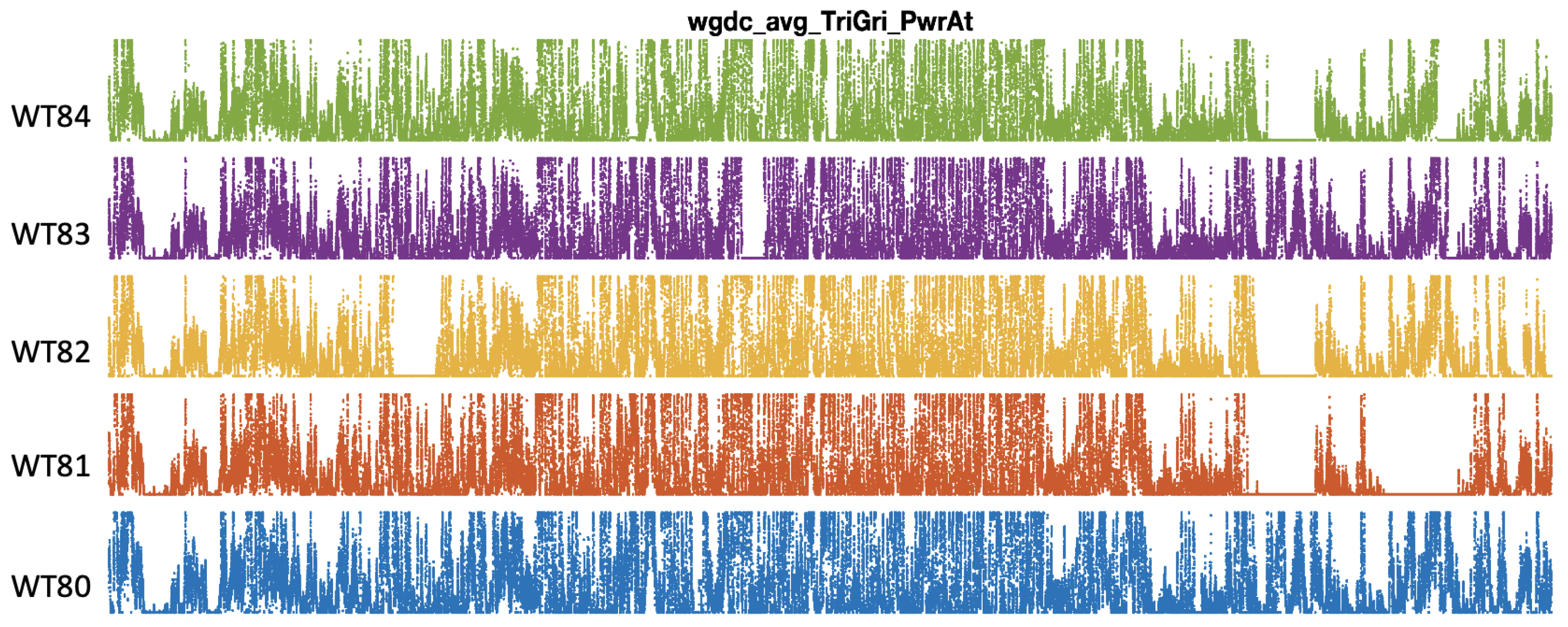Figure 1 shows the training portion of the wgdc_avg_TriGri_PwrAt signals, corresponding to the active power of each WT in the same temporal reference. The representation collects two-thirds of the total available signals. The third part is reserved for the test. Notice the strong similarity between signals, although it is occasionally observed that some WTs are not producing while the rest are.

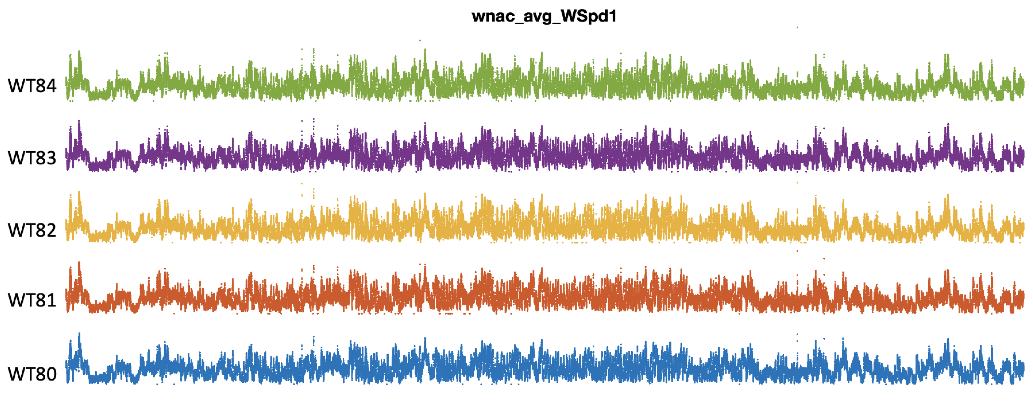
Figure 2 shows the training portion of the wnac_avg_WSpd1 signals, corresponding to the wind speed measured in the nacelle of each WT in the same temporal reference. As in Figure 1, the representation collects two-thirds of the available signals. We note the close similarities of the envelopes of the wind signals, much greater than the powers generated for each WT.

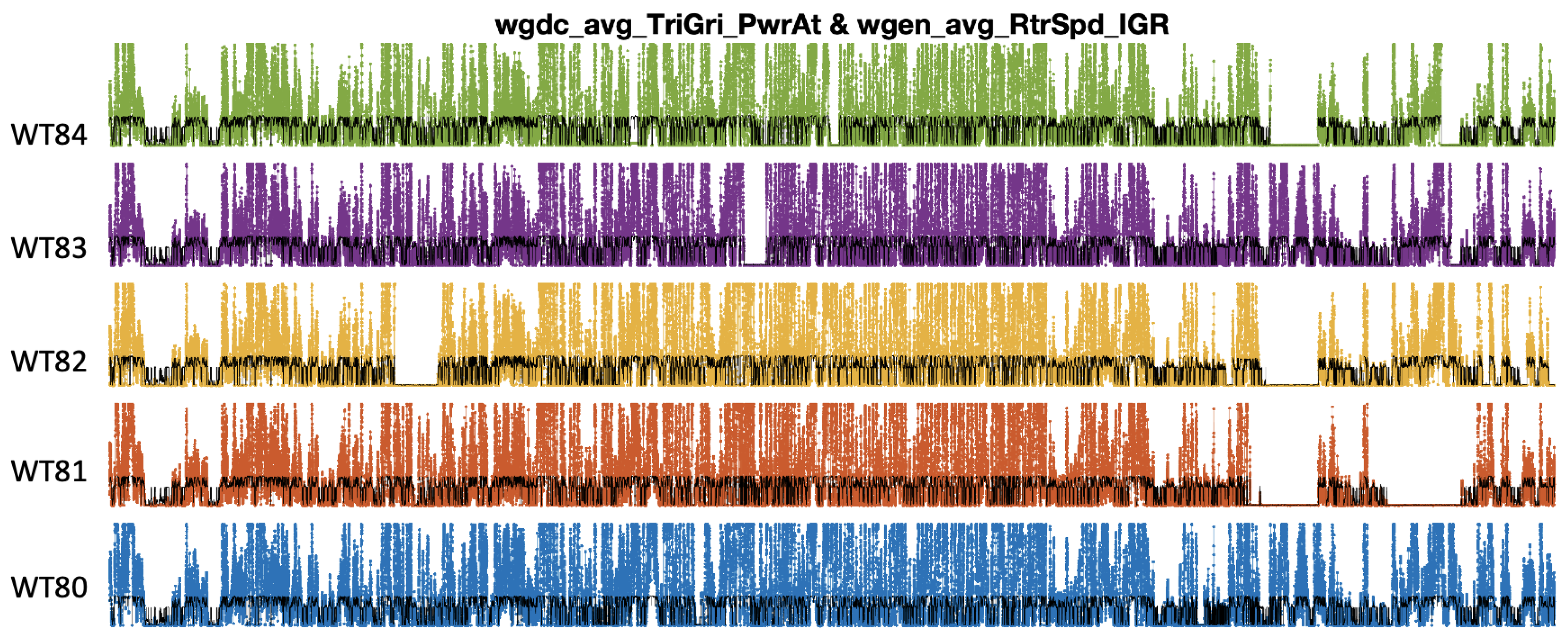
In Figure 3, for each WT, we superimpose over the signals wgdc_avg_TriGri_PwrAt the rotation speed of the rotors provided by wgen_avg_RtrSpd_IGR, which are represented scaled and in black colour, to confirm that in the intervals where power is not produced, the WT is indeed also stopped. So the data is consistent and reliable.

2.2. Fuhrländer FL 2500/100 power curve provided by the manufacturer

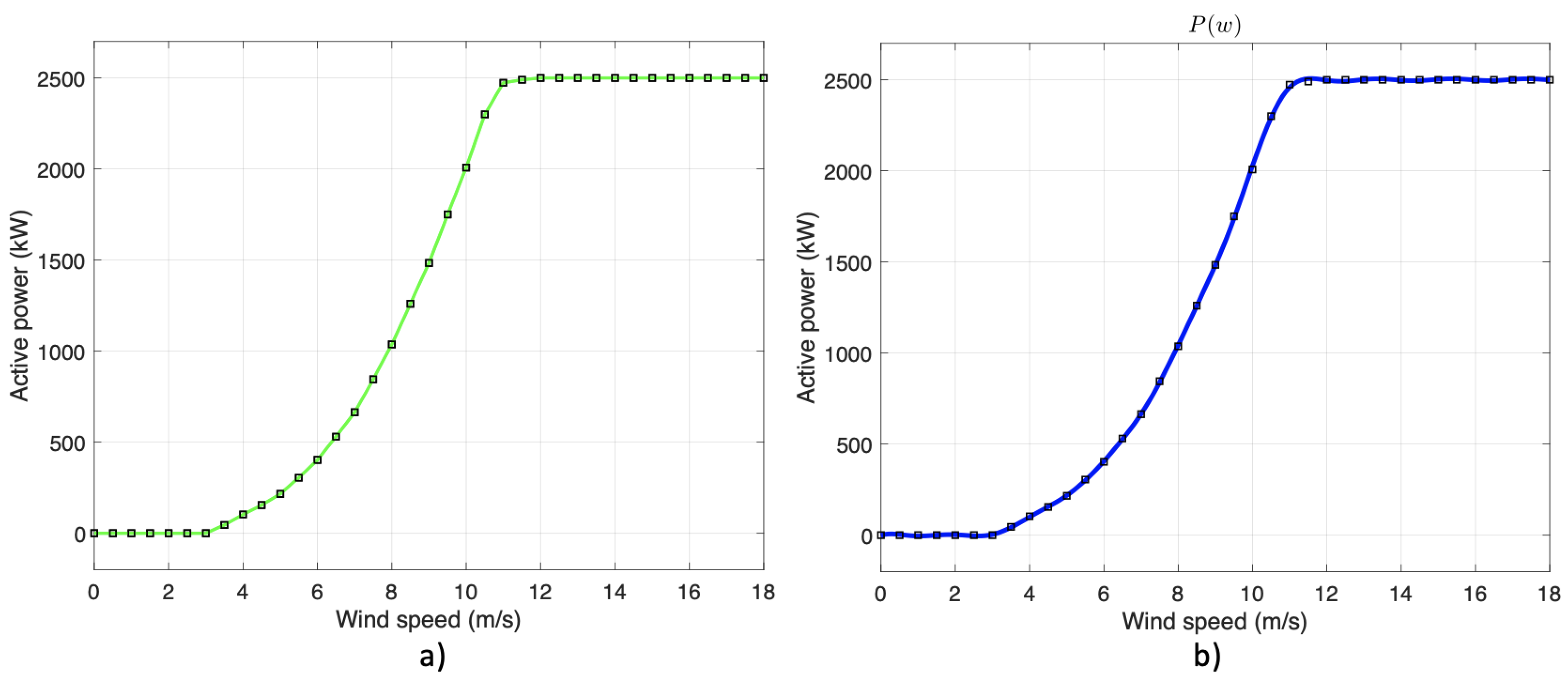
The Fuhrländer FL 2500/100 manufacturer characterizes the power generated with the wind speed of its WT model at increments of 0.5 m/s. One can find such data at https://www.thewindpower.net/turbine_en_154_fuhrlander_fl-2500-100.php.

These measurements were taken in a controlled environment. In the left graph of Figure 4, one can see the points provided by the manufacturer represented by small black squares. The green line connects the points with a straight line. Indeed, carrying out these measurements is expensive, so we need to manage the intermediate values between the given points. In the representation on the right of Figure 4, we show the continuous function used to have a power value for the wind speeds between the points provided by the manufacturer. So, we have found a continuous function that better adjusts the manufacturer’s points in terms of root mean squared error (RMSE). Previously, to decide the used curve, we compared techniques such as polynomial approximations of different orders, developments in the Fourier series, and even third-order splines to make this approximation. We discarded the third-order splines because we did not want to handle a piecewise function with such many parts. Of the contrasted approximations, the decomposition into sinusoidal functions is the one that provides better results in terms of RMSE, better even than the Fourier series for the same number of terms. Using sinusoidal functions, we have verified that seven sinusoidal terms obtain a better approximation than nine. For the approximation of the curve, we use the following expression:

P_{N} (w) = \sum_{i = 1}^{N} A_{i} s i n (a_{i} w + ϕ_{i}) .

(1)

where

P_{N} (w)

provides the power at the wind speed w. So, we particularize

P_{N} (w)

for

N = 7

. We represent the values of amplitudes

A_{i}

, frequencies

a_{i}

, and phases

ϕ_{i}

in Table 1.

2.3. Anomaly filtering

According to the distribution presented by these points, the anomalies, there are authors such as in [8] who classify them according to three typologies: (1) of power sensor failures, (2) wind speed sensors failure or (3) due to the starting and stopping effect of the WT.

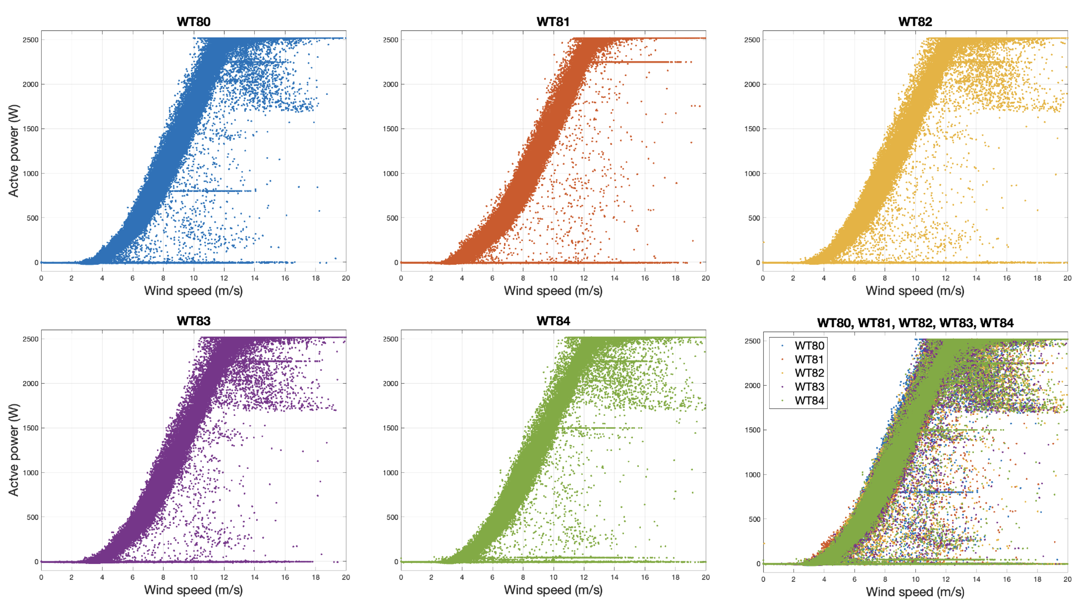
In Figure 5, we see represented the power curves of each WT resulting from directly crossing the wnac_avg_WSpd1 and wgdc_avg_TriGri_PwrAt signals provided by the SCADA. A total of 3/4 of the available signals are used. In some of these curves, anomalies appear, forming horizontal lines, which are attributed to failures of type (1), which are related to the power sensors. The anomalies distributed randomly inside the curves are of type (3), mainly attributed to the phenomenon of starting and stopping the WTs.

In any case, the anomalies introduce errors in estimating the wind power curves. Before the estimation of the power curves of each WT, it is necessary to filter them.

So, to filter the data of each WT, we use the continuous manufacturer’s curve approximated by

P_{7} (w)

given in (1) that we move horizontally to the right

w_{o f f}

and vertically down a distance

p_{o f f}

. Considering the signals wnac_avg_WSpd1 and wgdc_avg_TriGri_PwrAt at the point k to be

w_{k}

p_{k}

respectively, then if the following inequality fulfils, we establish tha

p_{k}

is an anomaly:

p_{k} < P_{7} (w_{k} - w_{o f f}) - p_{o f f}

(2)

We initially determine

w_{o f f}

and

p_{o f f}

empirically to 1m/s and 100W, respectively. Later on, we realize that small variations of such values do not affect the estimations.

Note that if

w_{o f f}

increases, we collect more points around the curve, but we can also enter some anomalies, mainly of type 3. Otherwise, maintaining a value of

p_{o f f}

of 100 allows us to collect the points of the curve that present slight measurement errors when the WTs are stopped or working at total capacity.

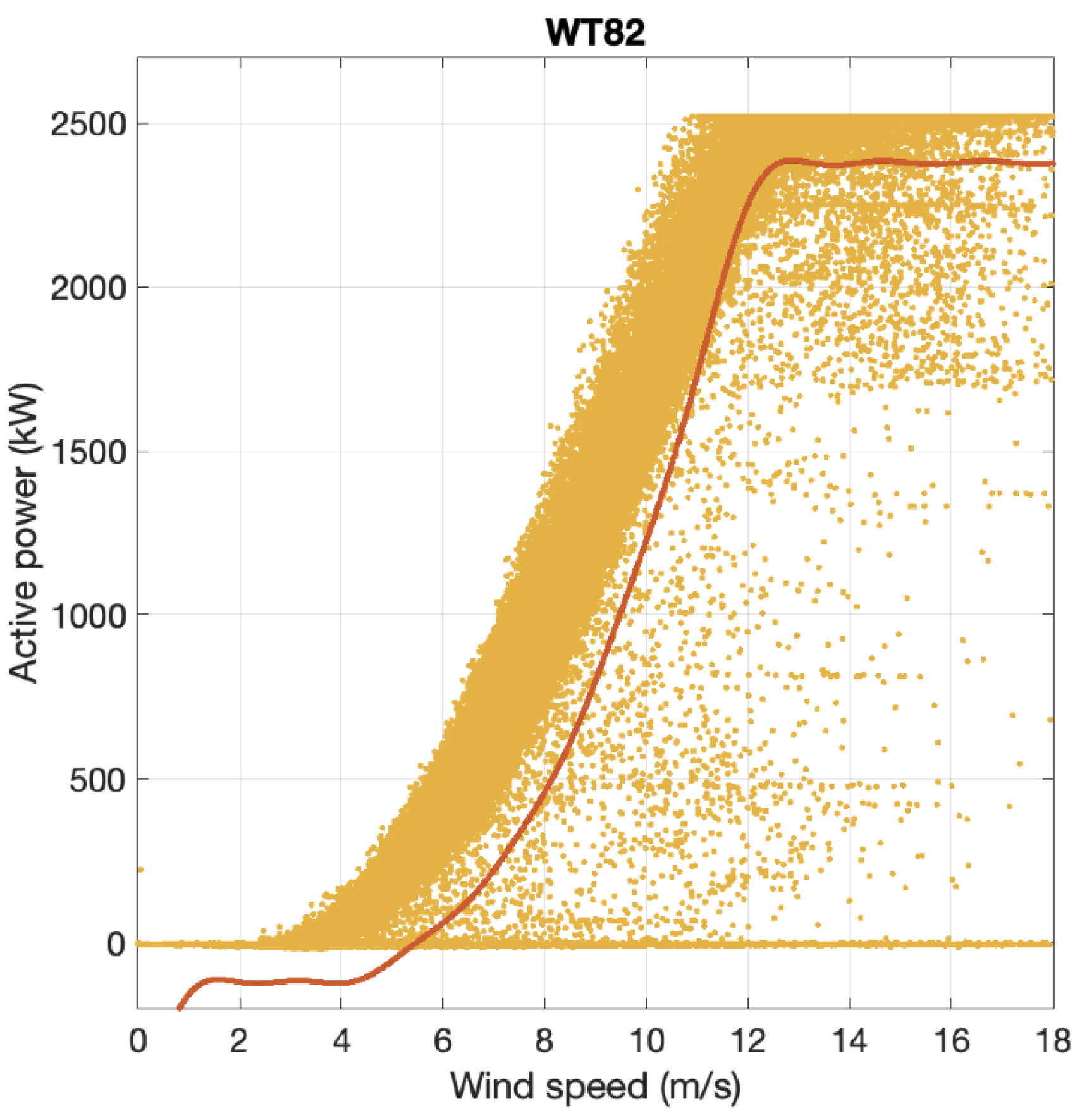
In Figure 6, we can see the graphic interpretation of the filtering rule where superimposed on the WT82 points, in red, is represented the function

P_{7} (w_{k} - 1.3) - 120

2.4. Wind Power curves estimation

Once the SCADA data anomalies have been filtered according to the rule described in the previous section, we estimate the wind power curve. Of all the existing non-parametric methods, we choose to use a classical neural network of relatively small dimensions since we understand that the filtering quality used to eliminate anomalies and clean the data used for the training has more influence on the results than the chosen method or increase the dimensions of the network.

Then, considering s the wind speed and

p (s)

the power for such s, the ANN model N hidden neurons takes the form:

p (s) = w_{o}^{T} σ (w_{i} s + b_{i}) + b_{o}

(3)

where the column vectors

w_{i}

and

w_{o}

of size N contain the input and output weights, respectively. The same size vector

b_{i}

contains the input biases while the scalar

b_{o}

contains the output bias. Function

σ ()

stands for the activation function, which, in this case, applies the hyperbolic tangent sigmoid to all the elements of its input vector.

We use the Levenberg-Marquard algorithm for training with 2/3 of the total available data. We chose N=10. The test will use the last third of the available data.

Once the network weights are calculated, p(s) provides the curve directly.

3. Results

3.1. Filtering and isolation of anomalies

This section presents the result of filtering anomalies according to the expression in (2). The same filtering values of

w_{o f f} = 1.3

m/s and

p_{o f f} = 120

W have been used for all WTs. In all Figures from Figure 7, Figure 8, Figure 9, Figure 10 and Figure 11 we show the same results WT to WT.

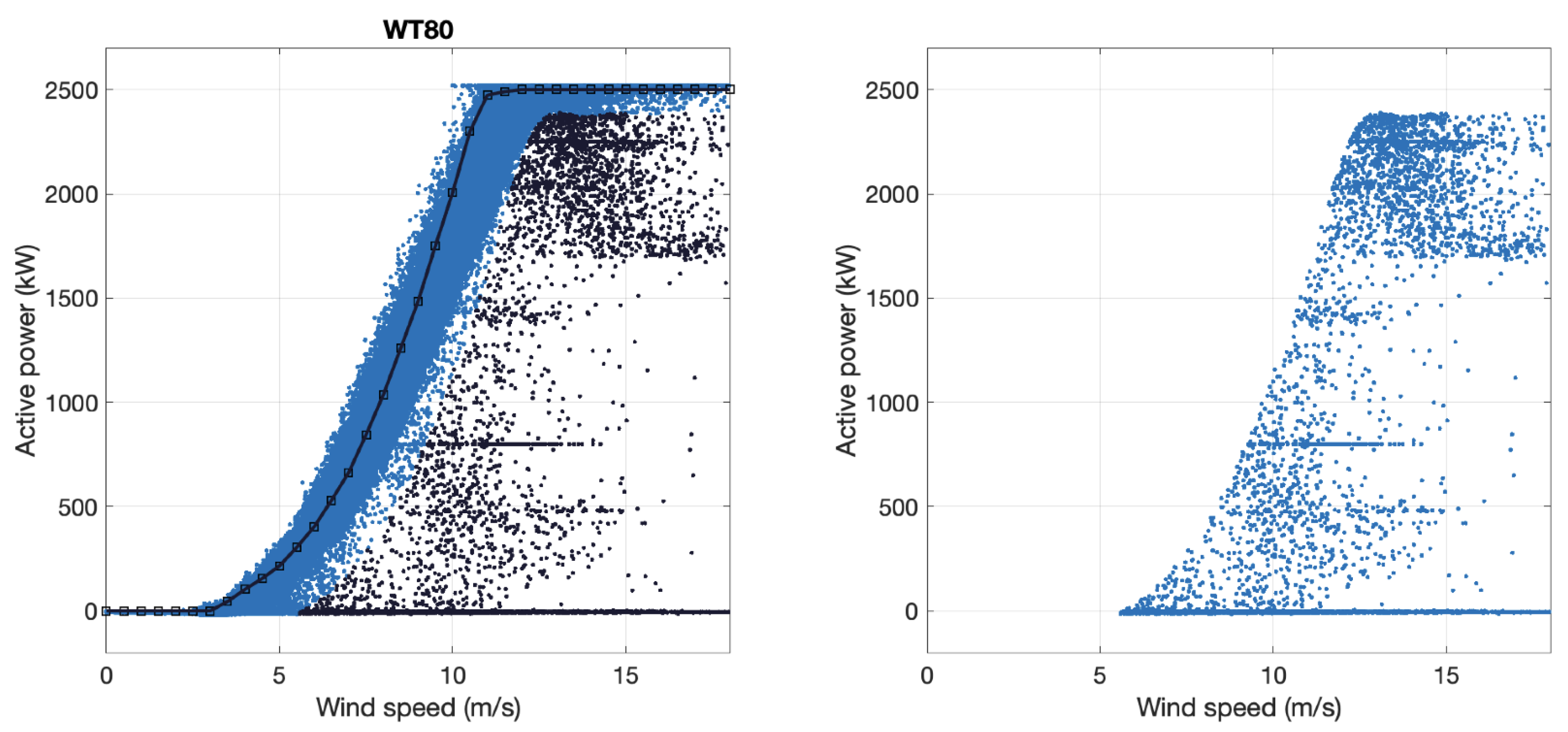
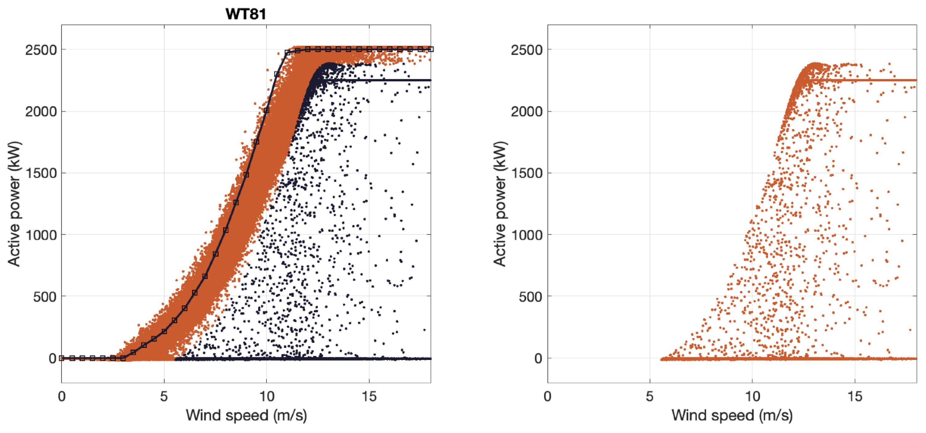
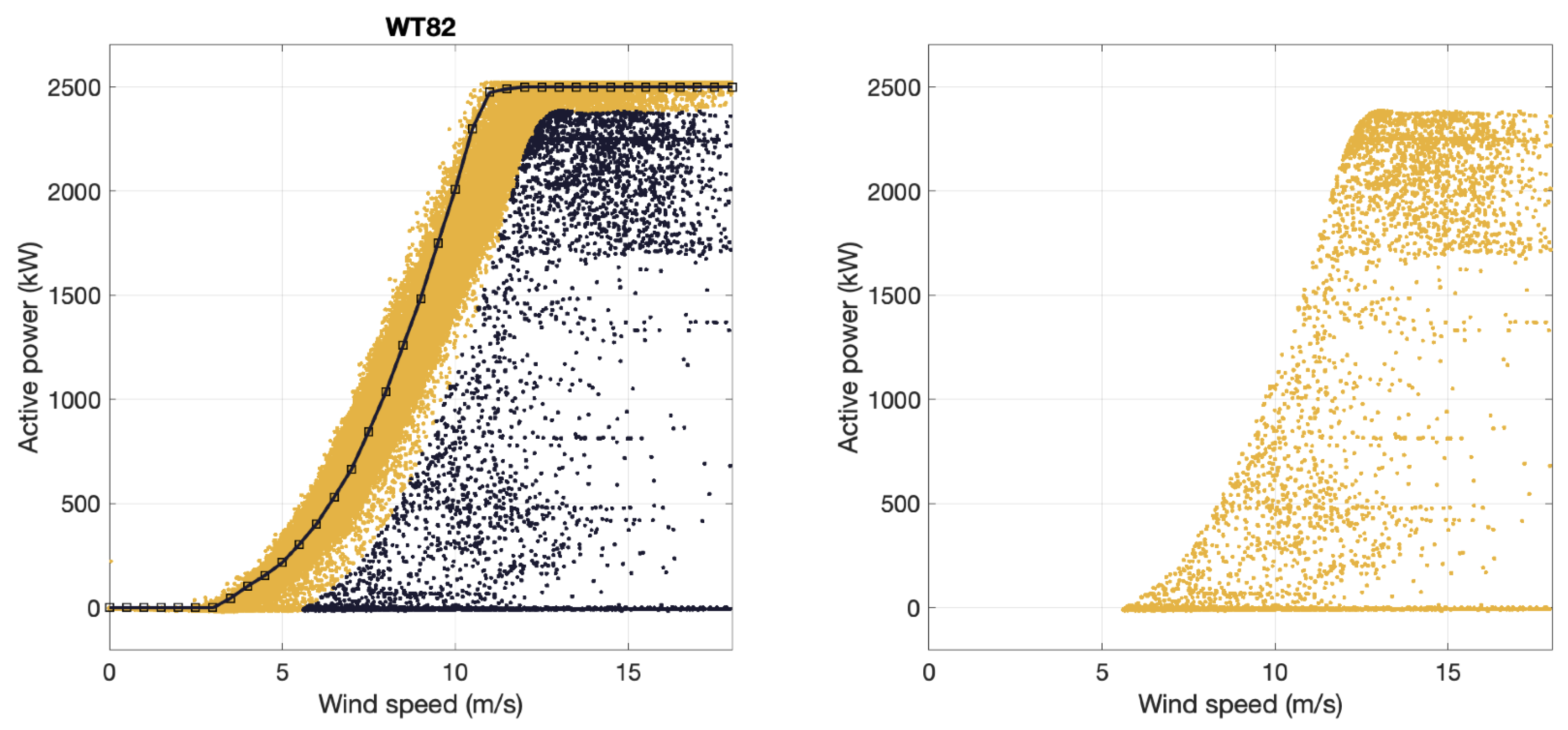
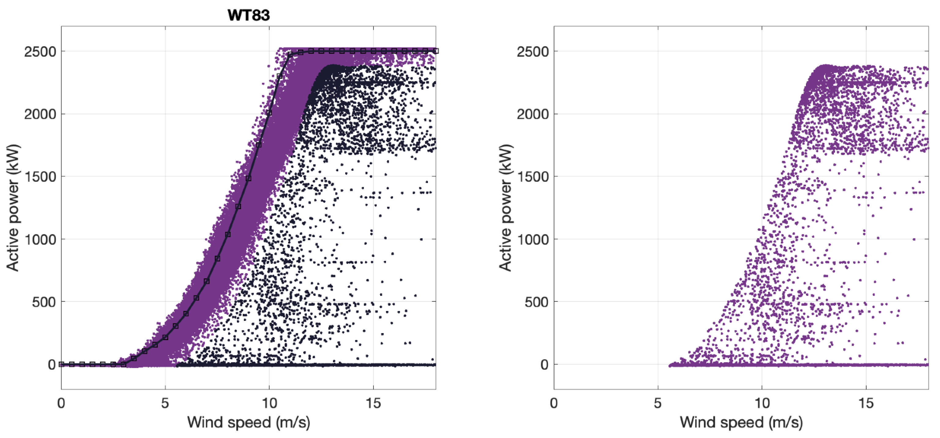
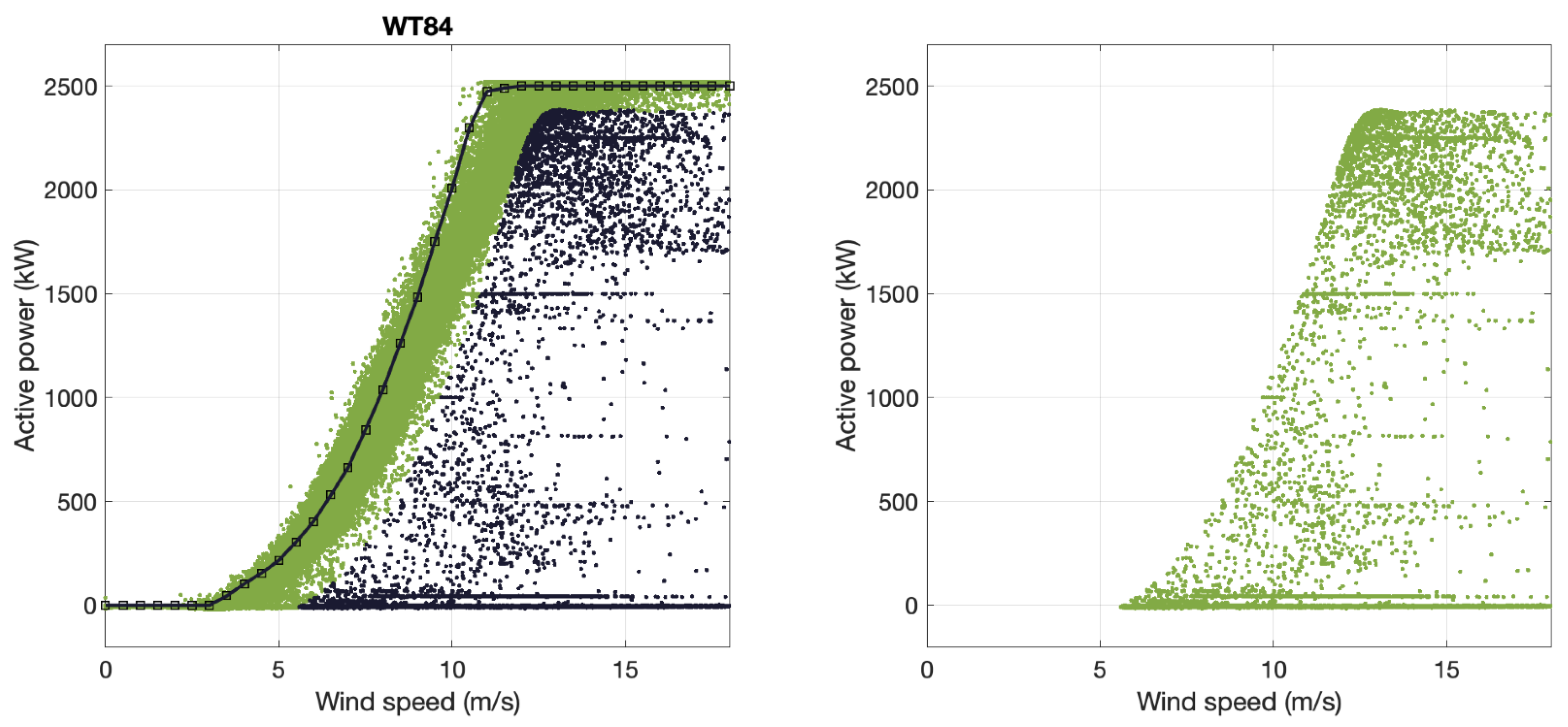
So, each figure shows the results for each of the 5 WTs of the WF individually. Notice that different colours identify the data of each WT. The points detected as anomalies in the left subplot are marked in black. On the colour points, we present the curve, also in black, provided by the manufacturer. In the subplot on the right, we represent the points captured as anomalies in isolation.

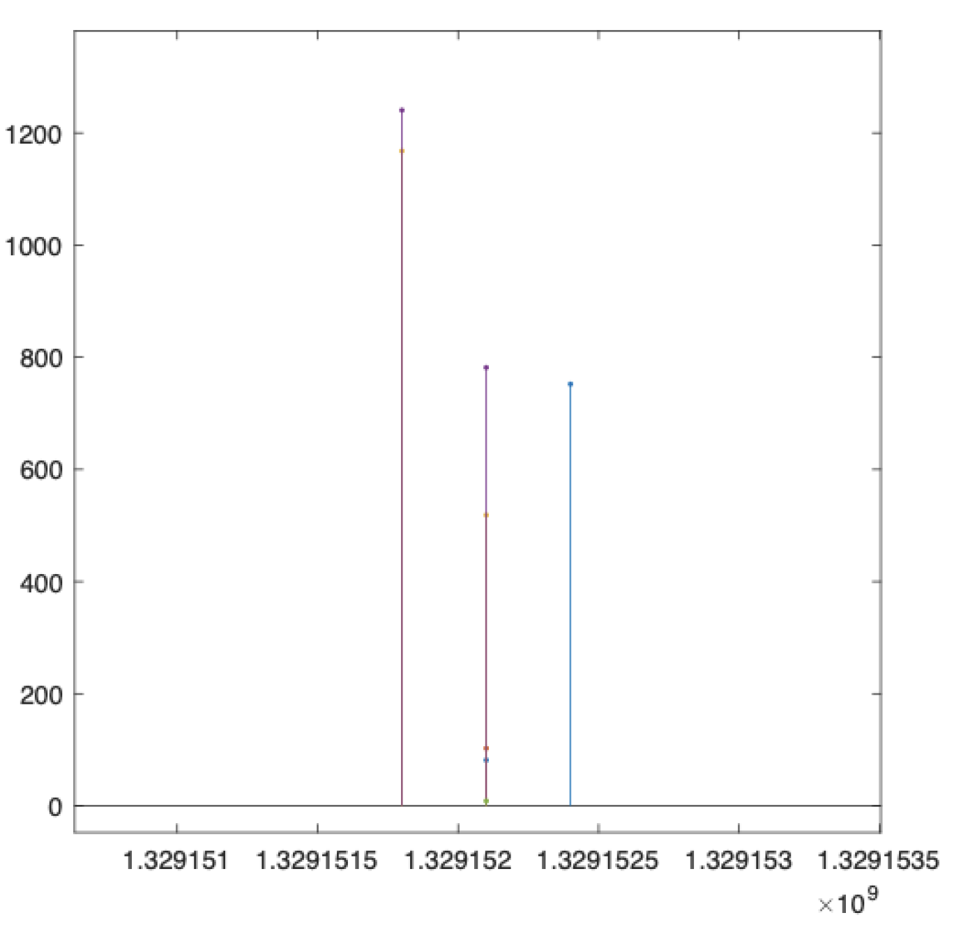
From these Figures, we notice a curiosity. The pattern of anomalies is characteristic of each WT. We note, for example, that the horizontal lines that usually draw the anomalies appear in different positions for each WT. The second observation comes from the temporal representation of these anomalies. That is, if we represent only the anomalies of the different WTs superimposed on the same temporal axes, as we have done in Figure 12, Figure 13 and Figure 14, we observe that anomalies tend to be concentrated in the same instants of time. Figure 12 shows a broader time scale, Figure 12 shows a more narrow scale, and Figure 14 shows a detail.

3.2. Using the filtered SCADA signals to estimate Power Curves. Training data

For each WT we estimate the wind-power curve using the ANN architecture described in (3) by using 3/4 of the total available data for the training by selecting the filtered wind speeds (wnac_avg_WSpd1) as the predictor and the filtered active power (wgdc_avg_TriGri_PwrAt) as the target. For all WTs we have used the same ANN size consisting of

N = 10

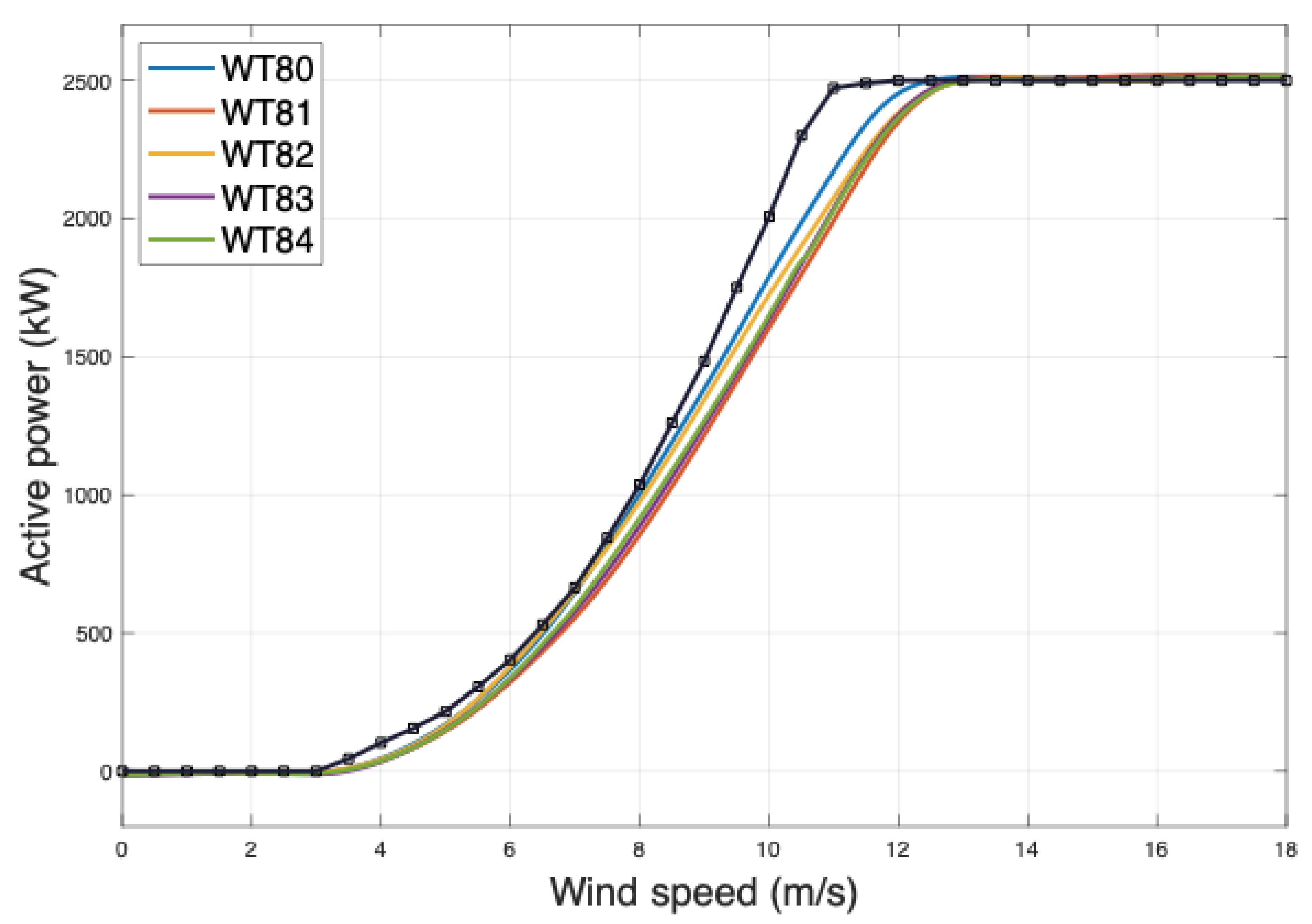
hidden nodes (neurons). Figure 15 shows all the estimated curves of each WT together with the power curve calculated from the data provided by the manufacturer in black indicating, in small squares, the specific points provided.

At this point, we notice how the estimated power-wind curves obtained from SCADA data differ from the one provided by the manufacturer, especially in the rang that goes from 8 to 12 m/s.

Comparing the estimated curves of each WT, we also notice that they are slightly different.

3.3. Using the filtered SCADA signals to estimate Power Curves. Test data

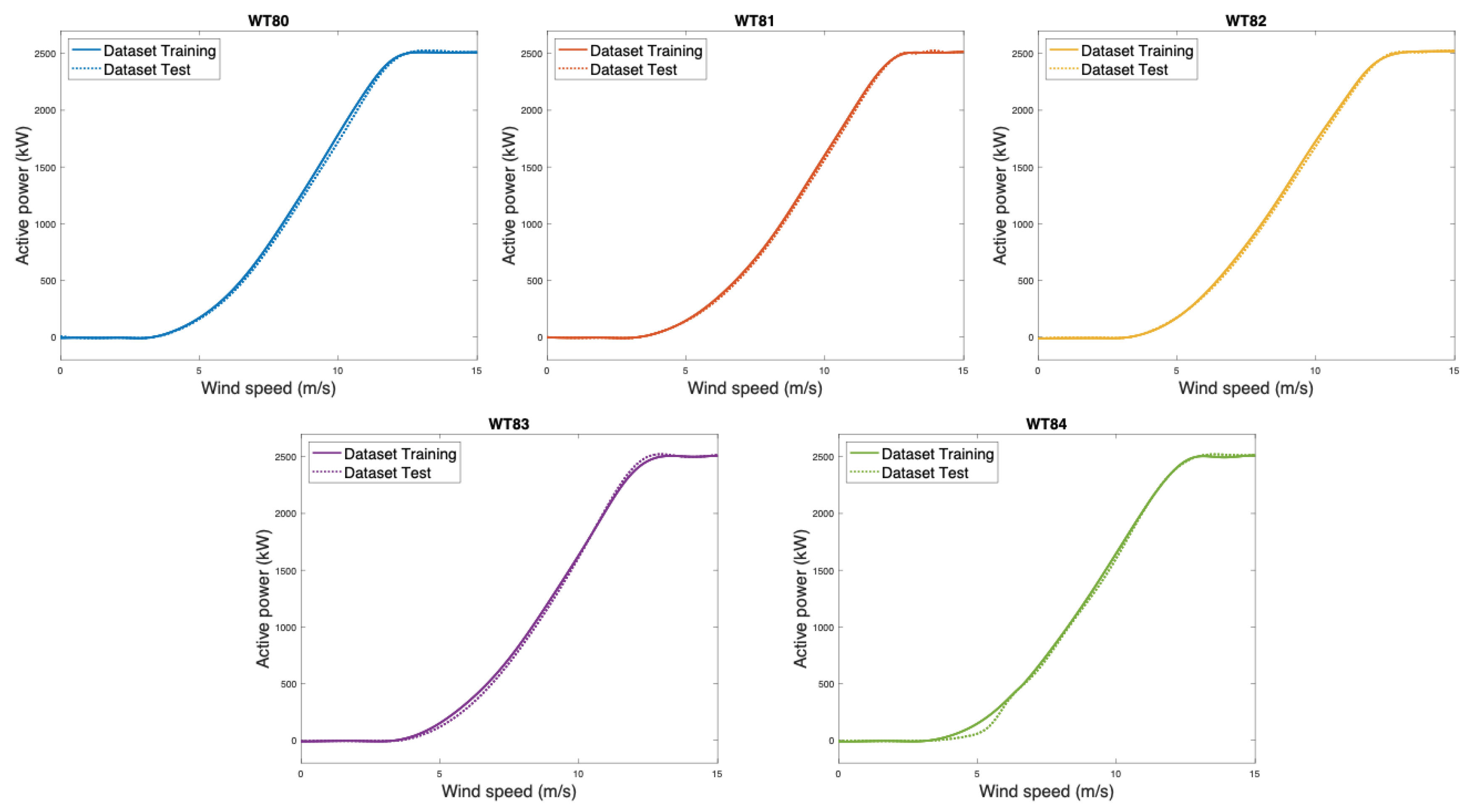
Using the same anomaly filtering and estimation method, in this section, we estimate the same curves from the last quarter of available data that we reserved for the test. Once estimated, we compare them with the curves obtained in the training part. We provide the results in Figure 16.

It is interesting to check that the estimated power curves of each machine in the test part fit very well with those obtained using the training data. The most notable difference is the WT84 machine, which suffered a major breakdown, causing it to be stopped for a long time. In this case, we see that the differences between the curves are observed in the part of the initial start-up of the WT when little power is still generated.

4. Discussion

We want to point out different aspects. In the context of this work, we understand by anomalies all those points that, due to failures in the sensors that measure the power or the wind speed or due to the starting and stopping processes of the WTs, fall in places far from the theoretical curve. Therefore, to obtain a good curve estimation, we note the need to filter anomaly data before the estimation to remove anomalies, as otherwise supervised ML-based methods also attempt to capture them into the models. So, when working with SCADA data, estimating the power curves of each WT from the data (cleaned of anomalies) is necessary since there are significant differences from the power curve provided by the turbine manufacturer. The cause of such significant differences seems to be the nature of the SCADA data, which consists of temporal averages, in our case, of 5 minutes. Instead, the manufacturer’s values model instantaneous relations of wind and power.

In this work, we use a filtering rule which depends on the choice of

w_{o f f}

and

p_{o f f}

values, which can slightly determine the estimates of the curves in the regions where the curve meets the flat areas. In any case, what is vital is to consider the same rule in both the training and test phases to clean anomalies in the same way. This rule can be refined by changing the estimate of the curve provided by the manufacturer,

P_{7} (w)

, to the estimate of the curve measured in each WT. As noted in our work, we have kept a general rule for all WTs.

Once the estimates are made, we see that, despite presenting significant similarities, each WT has its particular curve. In this sense, it is also interesting to see that, for each WT, the estimates made with the training and test data are highly similar for all the WTs that work correctly and for the one we know has a failure in the test part, the WT84, the malfunction is captured in its curve.

Regarding the study of anomalies, we want to highlight several aspects. Our study finds that anomalies occur at approximately the same time instants in practically all WTs, which, as a future idea, crossing the data between WTs could improve anomaly detection algorithms. The other idea suggested by the observations is that each WT presents a particular anomaly plot. As an idea for the future, it could be interesting to study the patterns of the anomalies and verify if focusing on their appearance, especially compared to WT, can be an advanced indicator of a possible problem.

5. Conclusions

Since the malfunction of WTs directly impacts their power production capacity, characterizing the relationship between wind and power has attracted much interest. This dependence, however, is complex and non-linear since factors of a very varied nature (mechanical, electromagnetic, aerodynamic, control systems, etc.) are involved. One powerful way to express this relationship is through the wind-power curve. From the result of this work, after analyzing 5 WTs of a small WF, we note, after the estimation of their power curves from SCADA data, that:

Estimated curves substantially differ from the curve that one can deduce from the data provided by the manufacturer.
Given that the locations of the WTs are not identical, the environmental conditions of each turbine are also slightly different. Consequently, the estimated curves for each WT reflect such differences and have slight differences.
Once the curve of one WT is determined from the training data, it is reproduced very accurately when re-estimated from the test data.
The anomaly filtering methodology introduced permits consistently estimating the power curves using simple ANNs.
When there is a problem in one of the WTs, such is the case of the WT84, where a fault is documented at one point in the test phase, the problem becomes visible in its power curve when estimated by test data.

Furthermore, thanks to the anomaly detection and filtering algorithm, we were able to verify that:

When we represent together the anomalies detected in each WT, it is observed that these tend to happen at the same time points and, usually, in all the WTs, very synchronously.
Each WT draws a particular and identifiable pattern of power curve anomalies, especially when we look at the bands of points that appear as horizontal lines on the power curve plot.

These observations suggest that future research should verify if a more focused study of anomalies can also be useful in terms of the prognosis of WTs. The occurrence of anomalies jointly for all WTs in a WF and representing them on power curves could provide a much faster prognosis than that provided by power curves alone, which need much more data for their consistent estimation and thus complement the information they provide.

Funding

This research was supported by the Ministerio de Ciencia e Innovación of the Spanish Government (ref: PID2020-120314RB-I00).

Data Availability Statement

The data can be extracted from the freely available database at: https://github.com/alecuba16/fuhrlander

Acknowledgments

The author would like to thank the Smartive company (http://smartive.eu/) for providing the data used in the experimental part.

Conflicts of Interest

The authors declare no conflicts of interest

Abbreviations

The following abbreviations are used in this manuscript:

ANFIS	Adaptative network fuzzy inference system
ANN	Artificial neural networks
GP	Gaussian Process
IQR	Inter quartile ranges
LSE	Least-square estimate
LSOM	Linear Self-organized maps
RMSE	Root mean squared error
SCADA	Supervisory control and data acquisition
SOM	Self organized maps
WF	Wind farm
WT	Wind turbine
WT80	Wind turbine 80
WT81	Wind turbine 81
WT82	Wind turbine 82
WT83	Wind turbine 83
WT84	Wind turbine 84

References

Yang, W.; Court, R.; Jiang, J. Wind turbine condition monitoring by the approach of SCADA data analysis. Renewable energy 2013, 53, 365–376. [Google Scholar] [CrossRef]
Sohoni, V.; Gupta, S.; Nema, R.; et al. A critical review on wind turbine power curve modelling techniques and their applications in wind based energy systems. Journal of Energy 2016, 2016. [Google Scholar] [CrossRef]
Wang, Y.; Hu, Q.; Li, L.; Foley, A.M.; Srinivasan, D. Approaches to wind power curve modeling: A review and discussion. Renewable and Sustainable Energy Reviews 2019, 116, 109422. [Google Scholar] [CrossRef]
Al-Quraan, A.; Al-Masri, H.; Al-Mahmodi, M.; Radaideh, A. Power curve modelling of wind turbines-A comparison study. IET Renewable Power Generation 2022, 16, 362–374. [Google Scholar] [CrossRef]
Bandi, M.M.; Apt, J. Variability of the wind turbine power curve. Applied Sciences 2016, 6, 262. [Google Scholar] [CrossRef]
Lydia, M.; Selvakumar, A.I.; Kumar, S.S.; Kumar, G.E.P. Advanced algorithms for wind turbine power curve modeling. IEEE Transactions on sustainable energy 2013, 4, 827–835. [Google Scholar] [CrossRef]
Wang, S.; Huang, Y.; Li, L.; Liu, C. Wind turbines abnormality detection through analysis of wind farm power curves. Measurement 2016, 93, 178–188. [Google Scholar] [CrossRef]
Moreno, S.R.; Coelho, L.d.S.; Ayala, H.V.; Mariani, V.C. Wind turbines anomaly detection based on power curves and ensemble learning. IET Renewable Power Generation 2020, 14, 4086–4093. [Google Scholar] [CrossRef]
Morrison, R.; Liu, X.; Lin, Z. Anomaly detection in wind turbine SCADA data for power curve cleaning. Renewable Energy 2022, 184, 473–486. [Google Scholar] [CrossRef]
Pandit, R.K.; Infield, D.; Kolios, A. Comparison of advanced non-parametric models for wind turbine power curves. IET Renewable Power Generation 2019, 13, 1503–1510. [Google Scholar] [CrossRef]
Li, S.; Wunsch, D.C.; O’Hair, E.A.; Giesselmann, M.G. Using neural networks to estimate wind turbine power generation. IEEE Transactions on energy conversion 2001, 16, 276–282. [Google Scholar]
Jang, J.S. ANFIS: adaptive-network-based fuzzy inference system. IEEE transactions on systems, man, and cybernetics 1993, 23, 665–685. [Google Scholar] [CrossRef]
Karaboga, D.; Kaya, E. Adaptive network based fuzzy inference system (ANFIS) training approaches: a comprehensive survey. Artificial Intelligence Review 2019, 52, 2263–2293. [Google Scholar] [CrossRef]
Raj, M.M.; Alexander, M.; Lydia, M. Modeling of wind turbine power curve. In Proceedings of the ISGT2011-India. IEEE, 2011, pp. 144–148.
Ouyang, T.; Kusiak, A.; He, Y. Modeling wind-turbine power curve: A data partitioning and mining approach. Renewable Energy 2017, 102, 1–8. [Google Scholar] [CrossRef]
Stephen, B.; Galloway, S.J.; McMillan, D.; Hill, D.C.; Infield, D.G. A copula model of wind turbine performance. IEEE Transactions on Power Systems 2010, 26, 965–966. [Google Scholar] [CrossRef]

Figure 1. Active power of each WT measured from the SCADA wgdc_avg_TriGri_PwrAt variable under the same temporal reference.

Figure 2. Wind speed measured in the nacelle of each WT provided by the SCADA signals wnac_avg_WSpd1.

Figure 3. Active power of each WT (wgdc_avg_TriGri_PwrAt) in different colours and a scaled version of their main axes rotation speed (wgen_avg_RtrSpd_IGR) in black, to verify the consistency o the SCADA data.

Figure 4. a) Points in (black squares) of the power curve provided by the manufacturer b) Continuos function

P_{7} (w)

in blue with the square points given by the manufacturer

Figure 4. a) Points in (black squares) of the power curve provided by the manufacturer b) Continuos function

P_{7} (w)

in blue with the square points given by the manufacturer

Figure 5. Wower curves of each WT resulting from directly crossing the wnac_avg_WSpd1 and wgdc_avg_TriGri_PwrAt signals. The last subplot is the superimposition of all the data of the 5 WTs.

Figure 6. Graphical interpretation of the anomaly filtering rule.

Figure 7. On the left, in black, the anomaly points of WT80 and the power curve provided by the manufacturer. On the right, the anomalies of WT80 are isolated.

Figure 8. On the left, in black, the anomaly points of WT81 and the power curve provided by the manufacturer. On the right, the anomalies of WT81 are isolated.

Figure 9. On the left, in black, the anomaly points of WT82 and the power curve provided by the manufacturer. On the right, the anomalies of WT82 are isolated.

Figure 10. On the left, in black, the anomaly points of WT83 and the power curve provided by the manufacturer. On the right, the anomalies of WT83 are isolated.

Figure 11. On the left, in black, the anomaly points of WT84 and the power curve provided by the manufacturer. On the right, the anomalies of WT84 are isolated.

Figure 12. Representation of the anomalies of all WTs in the same temporal reference. An extended temporal view is shown.

Figure 13. Representation of the anomalies of all WTs in the same temporal reference. A more narrow temporal view is shown.

Figure 14. Representation of the anomalies of all WTs in the same temporal reference. A few minutes of detail is shown.

Figure 15. Power curves of each WT estimated from the wind and power data reported by the SCADA system after removing the anomalies.

Figure 16. Comparison between the power curves estimated with the training and the test data for each of the WTs of the WF.

Table 1. Coefficients of

P_{7} (w)

Table 1. Coefficients of

P_{7} (w)

i	$A_{i}$	$a_{i}$	$ϕ_{i}$
1	4131.2000	0.1487	-0.2597
2	2199.6000	0.1909	2.8832
3	385.6073	0.5622	1.5075
4	86.5623	1.1268	1.9258
5	19.0806	2.1933	-3.3415
6	30.4685	1.6828	-4.1747
7	12.4781	2.7778	-3.2777

Disclaimer/Publisher’s Note: The statements, opinions and data contained in all publications are solely those of the individual author(s) and contributor(s) and not of MDPI and/or the editor(s). MDPI and/or the editor(s) disclaim responsibility for any injury to people or property resulting from any ideas, methods, instructions or products referred to in the content.

© 2024 by the authors. Licensee MDPI, Basel, Switzerland. This article is an open access article distributed under the terms and conditions of the Creative Commons Attribution (CC BY) license (http://creativecommons.org/licenses/by/4.0/).

Copyright: This open access article is published under a Creative Commons CC BY 4.0 license, which permit the free download, distribution, and reuse, provided that the author and preprint are cited in any reuse.

MDPI Initiatives

Important Links

Choose an area of interest and we will send you notifications of new preprints at your preferred frequency.

Disclaimer

Enhancing Reliability in Wind Turbine Power Curve Estimation

Abstract

1. Introduction

2. Materials and Methods

2.1. Data used

2.2. Fuhrländer FL 2500/100 power curve provided by the manufacturer

2.3. Anomaly filtering

2.4. Wind Power curves estimation

3. Results

3.1. Filtering and isolation of anomalies

3.2. Using the filtered SCADA signals to estimate Power Curves. Training data

3.3. Using the filtered SCADA signals to estimate Power Curves. Test data

4. Discussion

5. Conclusions

Funding

Data Availability Statement

Acknowledgments

Conflicts of Interest

Abbreviations

References

MDPI Initiatives

Important Links

Subscribe