1. Introduction
In 1989, [
1] already pointed to the increase trend in electric loads quantity and so power demand. Their work discussed many solutions, like use of dynamic pricing and time-of-use (ToU) tariff, that became reality in the years to follow. About 20 years later [
2] listed the same power demand concerns, adding to it a new player: the electric vehicle (EV).. The impact of EV on energy grid were also the main problem for [
3,
4]. Their research include scenarios with coordination of smart chargers. In the same paper, [
2], points to a lack in reliability of the traditional energy grid due to prospection of renewable energy sources and increase costs to maintain the transmission and distributions networks. The electric energy should be generated closer to its final consumer and a better communication framework needed to be built, as claimed in [
5] when the term smart grid (SG) was used for the first time. Nowadays, the transport sector is one major source of gas emissions. There are many challenges about modernizing and increase the use of public transportation and related to the transition from internal combustion to electric vehicles, which could not be considered gas emission free if the electric matrix behind it still based on natural gas or coal [
6].
In the context of SG, its evolution is fairly stated on the concepts of demand response (DR) and
demand-side management (DSM) [
7]. This last one reaches out the end user through tariff signals
offered by the local energy market, frequently named as critical peak pricing (CPP), real-time price
(RTP), and ToU [
8]. When a demand peak is identified, the hours related are charged with higher
price, this way users are persuaded to reschedule their appliances to reduce the bill. Legal deals with
energy suppliers and smart home controller (SHC) has been important instruments through which customers can optimize their energy consumption behaviors and achieve efficient management of the entire electrical network [
9]. A system grid view of the DR problem and their issues related to industrial scenarios can been seen in [
10,
11] reviews respectively.
The Brazilian National Electric Power Agency (ANEEL) classify the electric energy users into two groups: A, that are connected to the grid with voltages higher than 2.3 kV; and B, for voltages bellow 2.3 kV, included here are the residential consumers, classified as B1 [
12]. For the B1 group, two options of energy tariff are available: conventional tariff
, which is constant over time, and white tariff, which is subdivided into three hourly constant posts: peak post tariff
, intermediate post tariff
and off-peak post tariff
. Due to its continental size Brazilian energy market is subdivided into several regions, which each one could define their tariff values and post hours in consonance to the previous definitions. [
13].
Table 1 resumes both tariffs costs in official currency of Brazil for the local energy market closest to this paper authors [
14]. Note that there is no billing related to demand response or demand peaks covered by Brazilian official resolution [
12] for B1 group, but this work will take it into consideration due to its relevance for global scenario.
This work presents a new methodology to schedule home appliances in order to reduce the energy bill and maintain the user comfort when this variable is related to time shifting of the loads. By exploring some properties of Brazilian energy tariff we had decomposed the time axis into a geometric space in which the movement of loads through time could be mapped. Analytic analysis of this properties leaded us to find a specific point into the decomposed time space that assures relative lower cost and minimum load shifting. Benchmark trials in results section will show that the proposed methodology is about thousand times faster than classic algorithms used to solve this class of optimization problem and consumes substantially less memory resources that could lead to a future implementation into a small embedded system.
The remainder of this paper is divided as follows: Section two presents the literature review is. Section three discuss about load modeling and define study case scenarios. Section four states the SHC math model equations and constraints. Section five introduce the concept of tariff spaces and set its properties about geometric locus. In Section six we explain how the proposed methodology works and the simulations results are shown and discussed. Section seven will condense this works contributions and point some future assignments to improve it.
2. Literature Review
Currently, many studies have proposed solutions for energy efficiency in domestic environment due to the constant increase in both energy consumption and electricity tariffs. In a smart home (SH) scenario, home energy management system (HEMS) controllers are installed to schedule loads at times when the tariff is lower off-peak post [
9]. This scheduling typically take into account the user’s preferences and habits, which can lead to a direct confrontation with maximization of economy.
Considering the scenario with (un)interruptible loads under dynamic pricing, [
15] studied the scheduling problem using Markov decision process as possible solver. To provide a strategy of efficient management of electric energy and peak control in a domestic environment [
16] proposes the design of a SHC using binary linear programming. In order to deal with uncertainties with appliances use habits and renewable energy generation, [
17] propose a home appliance scheduler combining linear and stochastic programming. Concerned about load peak demand, [
18] modeled the appliances considering the worst case scenario and photo voltaic (PV) as negative load into CPLEX solver modeling the schedule problem as mixed integer programming (MIP). Considering the Day-ahead load scenario, a model of a house hold with PV system and including thermal controlled loads was proposed by [
19] which used quadratic programming to minimize the user cost.
Most renewable systems use batteries as energy storage unity which use should be modeled and constrained [
20]. This same author used two point estimation and gradient based particle swarm
optimization (PSO) to minimize cost and improve demand response in a HEMS. Diesel generators are also a common power source as considered in [
21] which used genetic algorithm (GAs) and linear
programming (LP) to model the trade between SHC and local distribution company. Both authors used stochastic models for modeling dynamic parameters.
The home appliances behavior is also a recurrent concern in this topic due to its unique and intricate characteristics. Subdividing a multiple stage load into a combination of virtual loads estimated by their peak energy consumption seems to be a reasonable way to handle this problem [
22]. Define polices based on weather [
23] or user life habits [
24] are also valid methods to optimize a HEMS.
However, loads reallocation can causes discomfort in the user’s habits and can trigger physical and psychological issues [
25]. Through time, many authors have proposed methodologies to balance the cost
vs comfort problem using different techniques like fuzzy logic [
25,
26,
27] integer programming [
28,
29], convex optimization [
30], GAs [
9,
31,
32,
33], PSO [
34,
35] and stochastic programming [
36,
37,
38], to quote a few relevant works.
The authors in [
39] propose an optimization-based DSM scheduler and energy controller for smart home considering renewable energy generation and battery storage systems to achieve reduction in energy cost, peak-to-average ratio in demand, improve user comfort in therms of thermal, illumination and appliance usage preference. Their Mathematical models are executed in many optimization algorithms.
The scheduling of appliances considering user habits can also improve the comfort issue. A Context-Aware Framework stated on a wireless sensor network to identify behavioral patterns and habits can generate recommendations that allows energy savings at homes [
40]. By monitoring rooms occupancy, a Multi-Agent System can analysis the house data and improve the energy consumption of heating, ventilation, and air conditioning (HVAC) systems [
41]. Analyzing patterns from user habits and PV generation a HEMS can avoid power peak consumption penalty [
24]. Noninvasive load monitoring approaches and a taxonomy of methodologies to optimize energy consumption has been reviewed by [
42].
The studies can be extended to smart builds or event to smart districts by using two level approach. The first level is described as the base unit of energy consumption, a SH with PV for example . The second level is composed by an array of base units in addition to shared co-generation and energy storage, for example: a residential building that each apartment has a solar panel on some windows and share also energy from a PV and/or wind turbine systems on roof [
33,
43,
44,
45].
In preparation for this work some relevant review articles related to topic where also found. The authors in [
46] identify research trends and patterns in building automation systems, describe sensors and actuators used to build HEMS and metrics for human comfort evaluation, mainly related to thermal [
47] and visual parameters ( daylight and glare). The coordination of HEMS due to rebound peaks, instabilities and contingents related to the high penetration of this kind of systems in energy grid is studied by [
48], which also lists coordination topologies and mechanisms, also implementations prerequisites and mathematical challenges. A comprehensive and in-depth systematic review of artificial intelligence (AI) based techniques used for building control systems, in therms of human comfort and energy efficiency has been studied by [
49]. A list of papers related to the use of HEMS for different conditions and cases depending upon multiple climate conditions, appliances, controllers with algorithms, distinct home occupants and their living style has been deliberated by [
50], which also identify the main components of HEMS and main optimization techniques to achieve appliances management. The review conducted by [
51] determine the primary purposes of smart home systems, listing their key features, characteristics and requirements, by identifying methods, tools and technologies to build such systems. By classifying into residential, commercial or educational, authors in [
52] provide an overview of the influential factors of energy over-consumption and if their loads should be direct or indirect controlled.
3. Load Model
During the bibliographic research, we could detect that there is no standard to load modeling or classification. Although many authors use similar therms like (non)controllable [
9,
25,
35], (un)interruptible [
18,
19], single/multi period [
22,
26]. In this paper loads are classified in two categories, following the stated in [
9]:
Controllable load (CL): loads that can be switched on/off for a certain period of time and are usually connected to the SHC. Examples of CL are: air conditioners, pool filter pump, non-programmable washing machine, dishwasher, iron or even outdoor lighting.
Detectable load (DL): these are non-controllable loads that can have their consumption estimated by the difference in the energy measurement of the smart meter (SM) and all others connected to a HEMS. Examples of DL are: audiovisual equipment; computer equipment; indoor lighting; toasters, refrigerator and freezer.
The parameters of the
load in a set that were used to structure the programmer model and simulations are presented in
Table 2, and are close related to scheduling problem modeling [
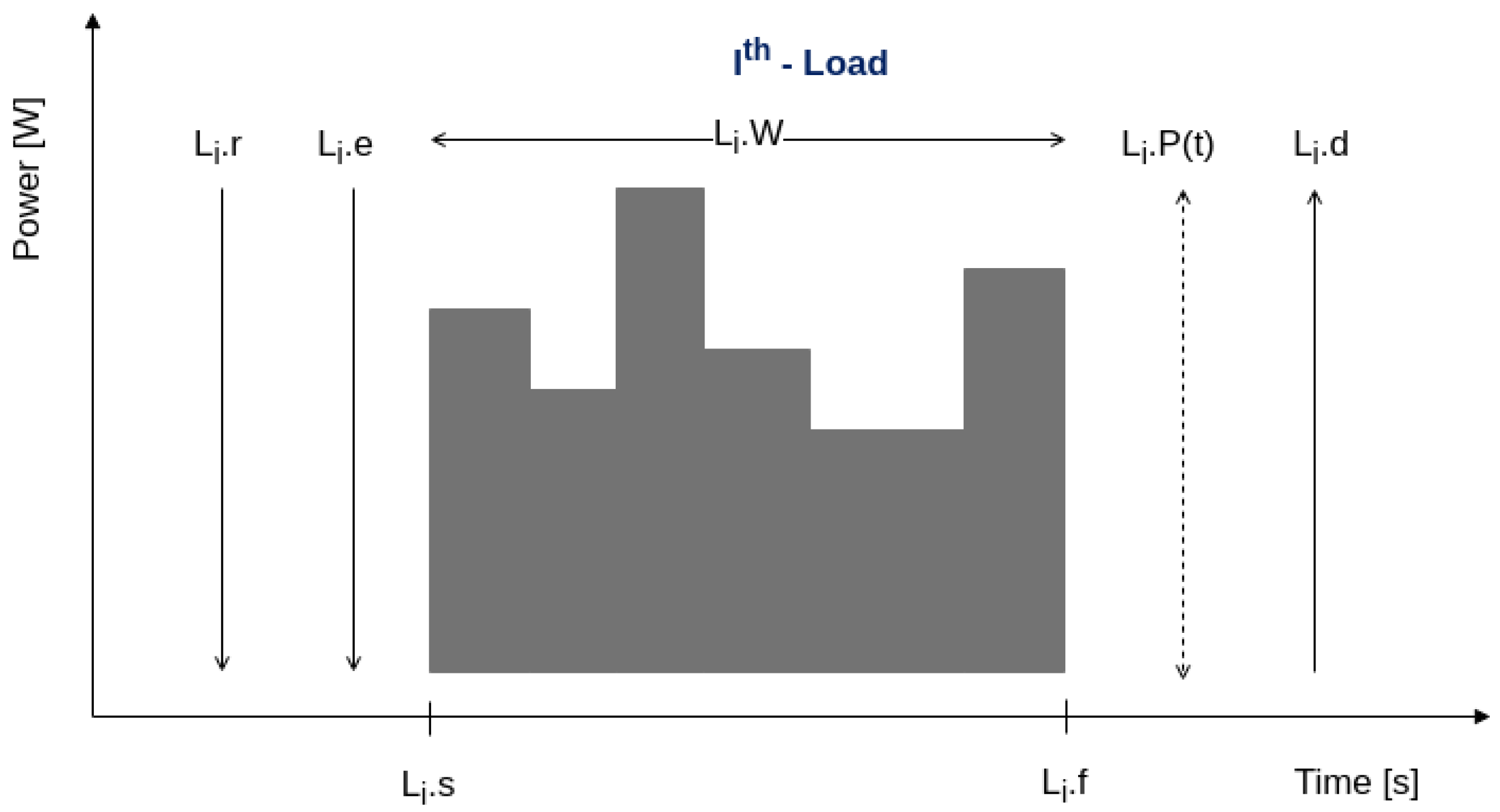
53]. An overview of the load parameters could be seem in
Figure 1. Details of the code that realize this structure in Julia language can be found in link at Appendix A.
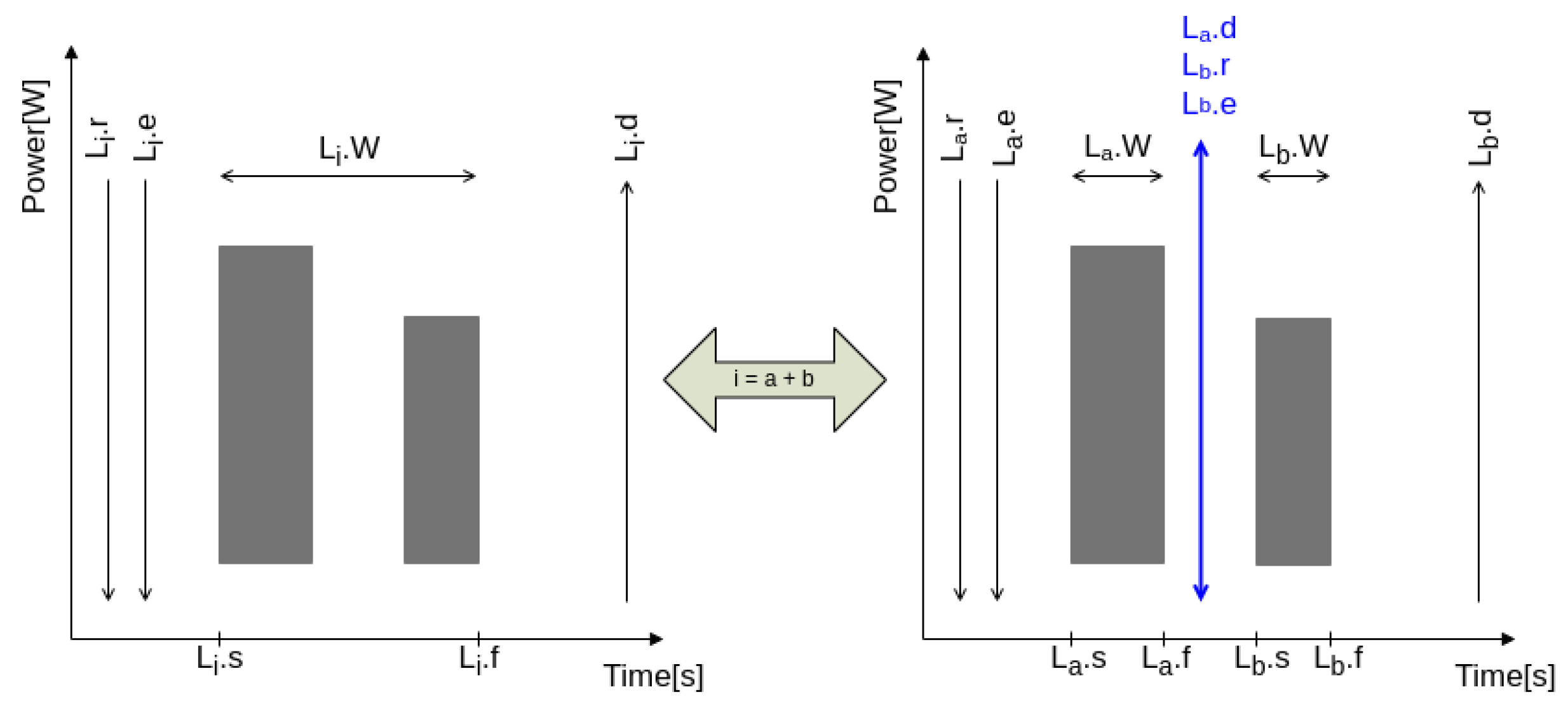
In this work we also considered that a complex or multistage load could be simplified as a combination of single small loads [
22]. In
Figure 2 is shown how this process could be done. The simulation step or sampling rate is also an important variable and should be considered as minimum as possible to achieve flexibility in scheduling [
23]. All simulations and benchmarks results were obtained using
. However, for some later illustrations it will be stated as
for better graphical comprehension.
Simulation Scenarios
Nine simulation scenarios are proposed in this work. The first one is related to a real house described in [
29] and also studied in [
9,
25,
35]. The details of appliances are described in
Table 3. This set of loads has been considered due to known results from previous works, working as a compass to assure the methodology presented in this paper.
The last eight load sets were random generated and used to collect benchmarks of execution time and memory usage for different quantity of loads, respectively: 10, 25, 50, 75, 100, 250, 500 and 750. This values were chosen to test impact of sets growing over the performance parameters. All benchmarks output details are described in a GitHub link in appendix A.
The characteristics common to all simulation scenarios are: a) sampling rate
; b) daily demand threshold:
for each set of ten loads, represented by an inverted Gaussian centered at 18:30h with an negative amplitude of
to simulate a decrease in the demand threshold to accommodate the DL; c) the ToU tariffs. For each load in any random scenarios the restrictions from Equations (
1) and (
2) were applied.
4. SHC Classic Model
The SHC receives information about utility billing, white tariff () and constant tariff (), controllable residential loads set (), residential load activation preferences (, , ), and comfort level (). For this purpose, the data comprising the residential loads, consumption profile () and the residential comfort profile () are modeled, leading to an appreciation of consumption, savings and comfort by a day-ahead load schedule.
4.1. Cost Model - f1
This paper uses the mathematical definitions of residential load at the grid level similar as presented in [
16,
29,
43]. The mathematical model of residential loads corresponds to Equation (
3) considering the following premises:
M schedulable loads,
N daily samples, and a sampling rate
, as well as the notation described in Load Model Section.
subject to the following constraints:
The constraints of Equation (
4) state that the schedule for activation of the
load must be within the minimum and maximum flexibility intervals defined by the user, while the loads must not exceed the threshold demand at the
time of activation according to the constraints of Equation (
5).
The cost function (
) defines the economic savings due to SHC normalized by the cost in constant tariff. The first and second terms in Equation (
6) correspond to the costs resulting from the user preference profile and the SHC scheduling, respectively.
where
so that the schedule proposed by the SHC is accepted by the algorithm as a valid solution for the user.
4.2. Comfort Model - f2
The comfort model adapted from [
29,
43] considers the comfort relevance level of a load
i as a fixed value and defines user preferences. For this purpose, the user should register the residential loads that can be scheduled in SHC, as well as the comfort relevance values (
) and the load on set times in terms of minimum (
), maximum (
), and preferred (
) values.
Equation (
7) represents the comfort function. The first term corresponds to the activation window of a load
i with respect to the user’s preferences, so this value is used as a reference for calculating the normalized comfort. The second term defines the distance between the time instant (
) selected by SHC and the time preferred by the user (
), which is weighted by the comfort relevance of the
load.
For a given load i with a comfort relevance of , this parameter takes the maximum value when the SHC’s scheduled time converges with the user’s preferred time (). Otherwise, if or , at the other end of the load activation window) the comfort will be minimal, since the operation cycle will start at the time farthest from the one the user has specified as the preferred time.
4.3. JuMP and Hierarchical Algorithm
Julia Modeling Language for mathematical optimization (JuMP) is a modeling language [
54] that condense a collection of supporting libraries and packages running in Julia language [
55] that makes prone to formulate and solve different problem classes related to optimization. The Multi-Objective Algorithms package [
56] provides many classic implementations ready to use. The best benchmark results were achieved with Hierarchical algorithm.
The Hierarchical multi-objective algorithm is organized in a way that returns a single point via an iterative scheme. First, it partitions the objectives into sets according to the objective priority. Then, in order of decreasing priority, it formulates a single-objective problem by scalarizing all of the objectives with the same priority using equal weights. Next, it constrains those objectives such that they can be at most relative tolerance worse than optimal in future solves. In other words, it solves the model up to a given MIP gap to obtain an optimal value for the first objective function, then solves, given the model restrictions, the second objective using the first set of values to constraint the feasible set of next optimization such the evaluated solution cannot get worse than first taking account some predefined tolerance. Finally, it steps to the next set of prioritized objectives. The solution is a single point that trades off the various objectives. In order to save memory space, the implementation of this algorithm in JuMP development framework does not record the partial solutions that were found along the way. [
54,
57,
58]. All code related to implementation of SHC Classic Model can be found in link at Appendix A.
5. Tariff Spaces
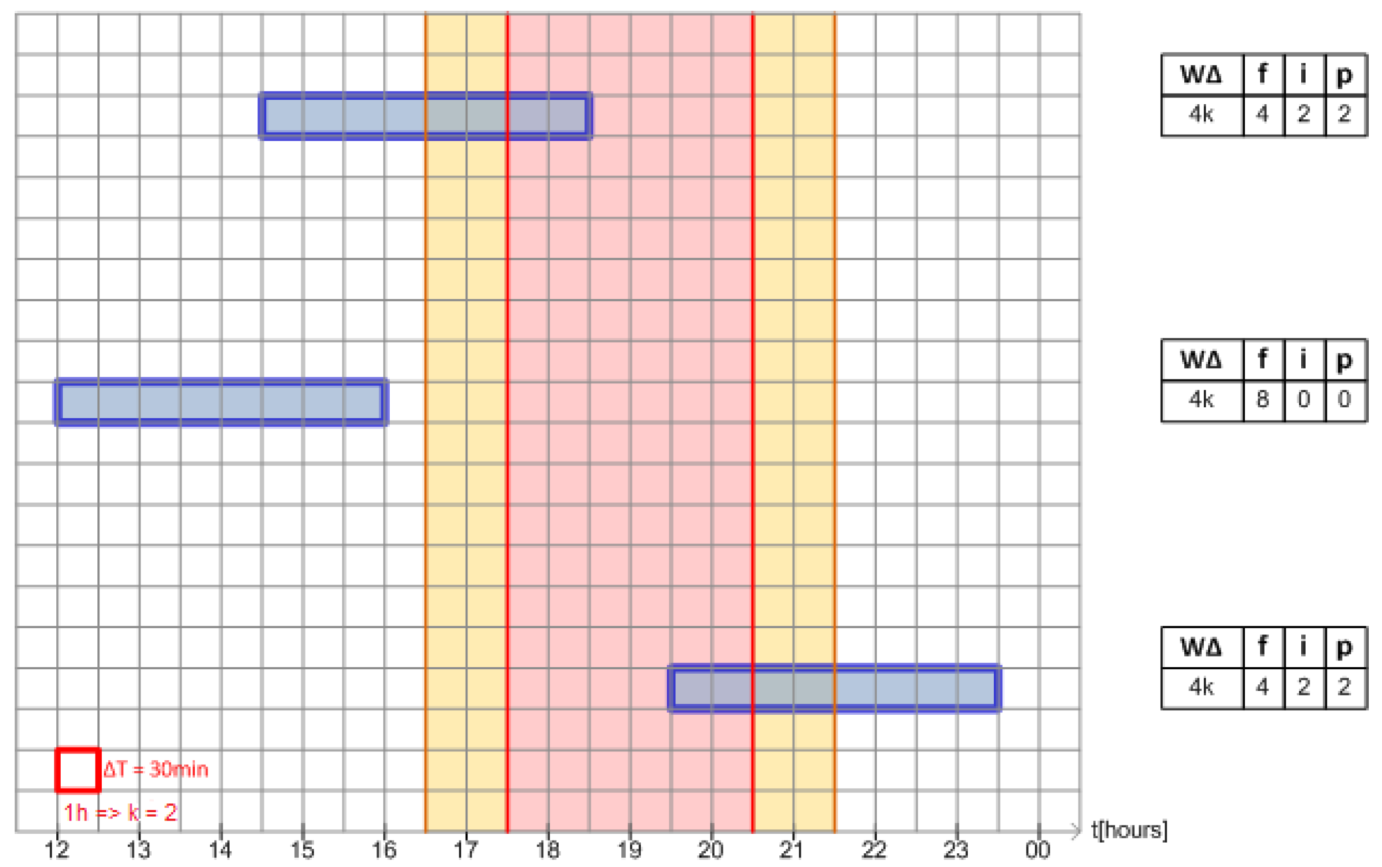
The reader is now invited to look at
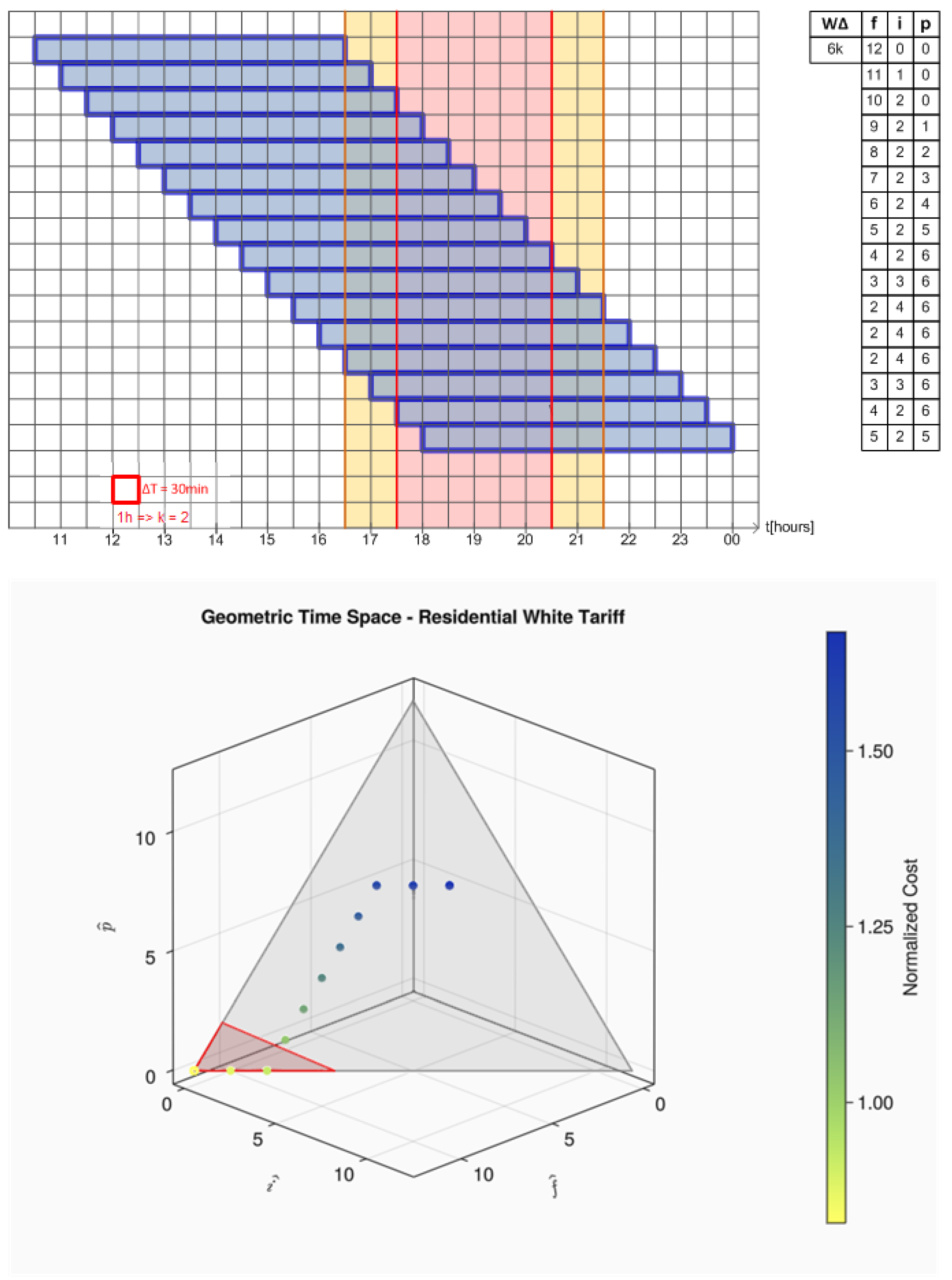
Figure 3. The squared chart represents a zoom around peak post of white tariff over time. The white outer regions are related to off peak post. The two thin yellow regions are related to intermediate post and the central red area represents the peak post. Each square along the chart represent a sample period which, for didactic purposes, it has been set to 30 minutes. The long blue rectangles represents a generic four hour long load started in three different instants. Note that while the four hours long load cross the tariff posts it is possible to evaluate how many discrete samples fit in each time post. These quantities are shown at right side of each load representation in
Figure 3.
From now, we assume that each time (or region) post in white tariff could be modeled as an independent dimension so that we could create a three dimensional vector with components (
) respectively to white tariff off peak post, intermediate post and peak post, whose lengths are the load length portion that fits inside of each post region. This vector space is named here as
Tariff Space. The process for a load
L that quantify how many discrete samples will fits in each time post accordingly to load length (
,
) and its start time (
) is defined as
time decomposition into tariff space whose output is a vector in Tariff Space, like the ones stated in right side of
Figure 3.
The code related to time decomposition into tariff space and its reverse operation can be read in link at Appendix A. As the vector resulting from time decomposition has been stated, we now can evaluate the cost of a load into white tariff scenario as a dot inner product:
where:
is the average power of a load and
k is the discrete amount of time related to one hour due to sample rate
t. All this symbols were defined in
Table 2. The values in vector
represent the white tariff post costs, as previous stated in
Table 1.
The minimum, maximum and normalized costs of a load can also been written as:
Note that maximum is a relative value and is evaluated using constant tariff value, due to our goal is to reduce bill relative to this reference value.
As cost margins has been defined, we now can analyze the extreme points of Equation (
14). Solving the equality at lower bound, we find the expression seen in (
15) which means that, to achieve this threshold the total load length should be into off peak post or, in other words, the point (
,0,0). Solving the equality at upper bound, we find the two points expressed in (
16). This three points delimits a region into tariff space in which the cost of a load in white tariff scenario is less or equal to constant tariff. Also note that Equation (
9) is in fact a equilateral triangle that represents all possibilities of combinations for (
) limited to
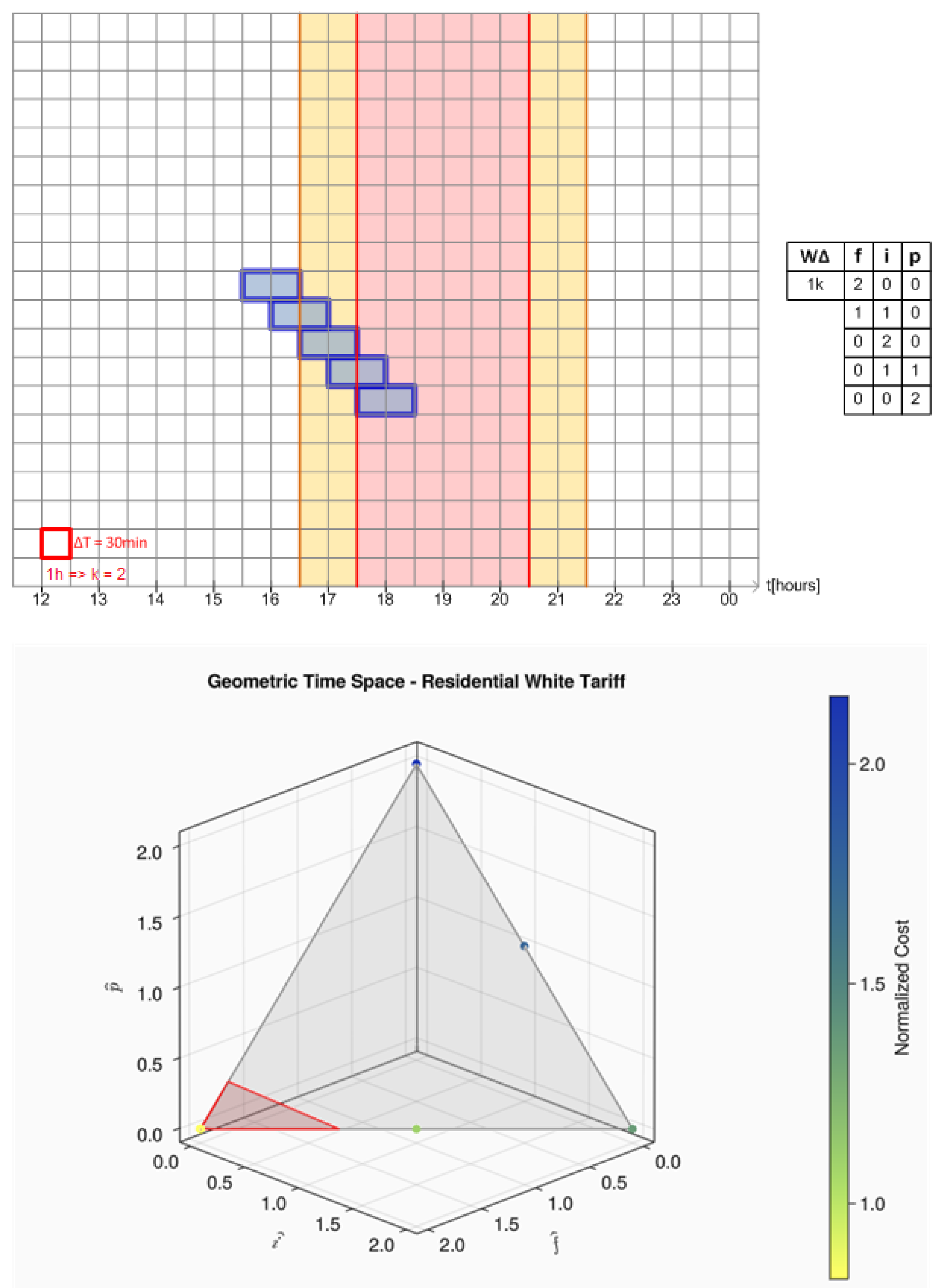
. All this regions plus the points related to an one hour long load crossing the tariff regions can be seen in
Figure 4. The points related to the load movement have been colored according to their normalized cost, so the reader can see how their price change over the gray triangle plane surface. The region delimited by a red triangle represent the lower cost region.
Observe that the one hour load "walks" through the side of the triangle only. That’s because time decomposition for this load would never have three components as its length fits alone into all three tariff regions or between its adjacent transitions by pairs. For loads with length less then or equal to only the vertices of the triangle should be seen.
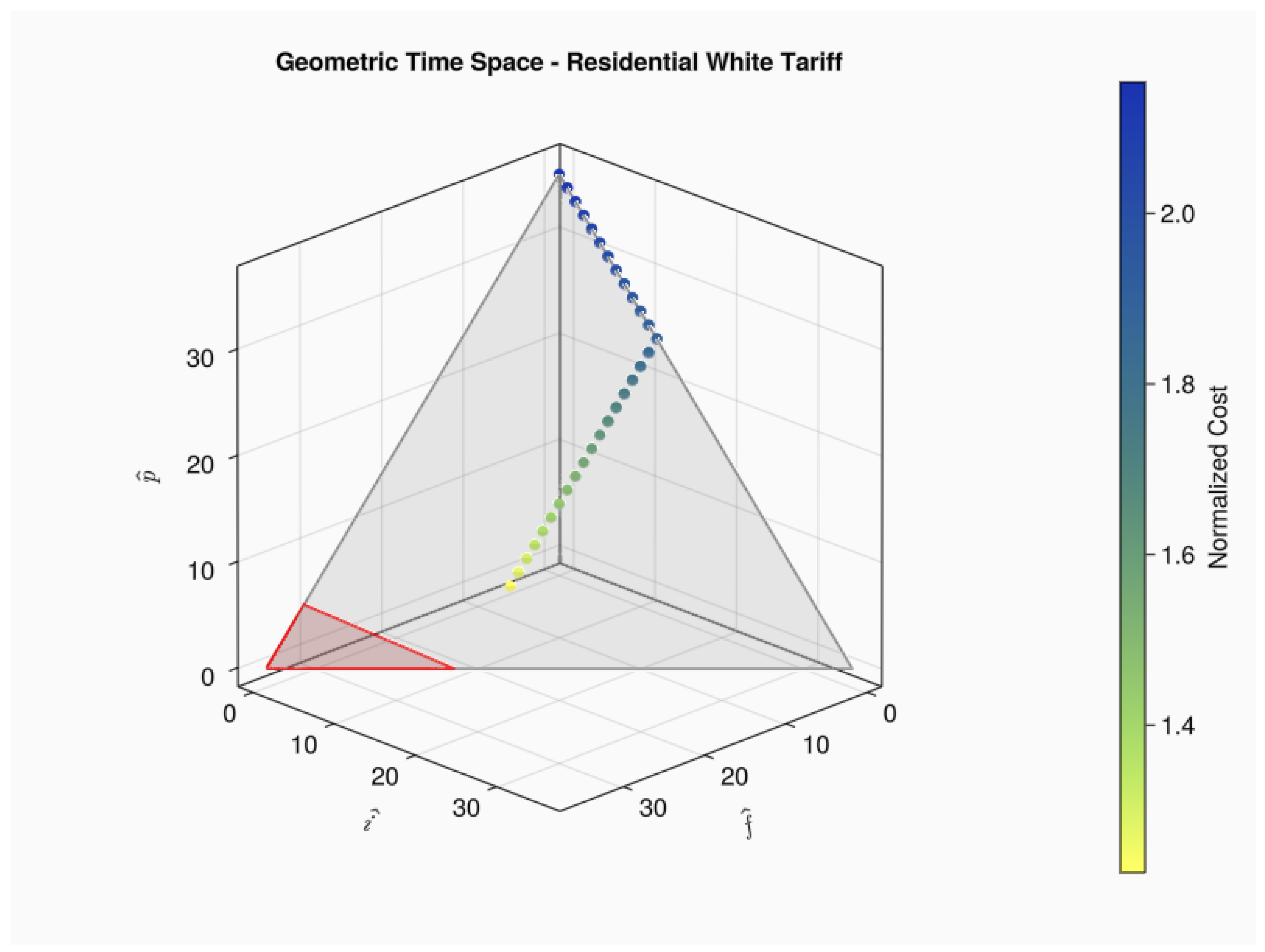
The next relevant load movement graphic is shown in
Figure 5 and represent a six hour long load. Note that behavior in tariff space is quite different of the observed in
Figure 4. In fact, this behavior can easily be modeled accordingly only to the load length. Those patterns, called here geometric locus of a load, are shown in the six equations that follows. More load decomposition into time space examples could be find in link at Appendix A.
The points shown in Equation (
17) are related to a load whose length is less or equal to
, as mentioned before. In Equation (
18) is represented a triangle side that connects axis
to
and is a linear trade off for a load whose length is lower or equal than an hour. A similar case occurs in Equation (
19) that represents the triangle side that connects axis
to
.
The Equation (
20) is applied when the load length is greater than an hour but less or equal than four hours and represents a parallel line to triangle side that connects the axis
to
. Note that, while a load longer than an hour crosses the intermediate post, that component remains constant and equal to an hour size (
k variable, defined in
Table 2). Also note that is a triangle side that could never be reached as we could not split a single load in two parts. As stated in load model section, multiple stage loads should be modeled as an array of single indivisible loads with shared deadline/release time.
The last two Equations (
21),(
22) are related with loads whose length are greater than 4 hours. Note that as a 4 hours or longer length loads cross the intermediate and peak posts their respective components should remain constant and equal to the regions occupied. Equation (
21) models a line parallel to a side that connects axis
to
. Finally, Equation (
22) is actually a single point into tariff space that exists while the load is placed through the three time posts and also larger then both intermediate and peak posts.
6. Proposed Methodology
Once we have defined all possible geometric locus for an appliance, it is pretty visible that only the lines defined by Equations (
19) and (
20) could reach the lower cost region. The analysis of upper bounds in Equation (
14) give us two points that could be combined to generate a parametric line Equation (
23). The intersection between this line and load geometric locus will give us the solution to our schedule problem,
where
is the parametric variable for Equation
23
Equations (
19) and (
20) can also be rewritten in parametric form,
where
and
are parametric variables for Equations
24 and
25 respectively.
Evaluating the interception point between Equations (
23) and (
24) we find a point described in Equation (
26) which is one of the points that belong to ones listed in Equation (
16). Graphically it is indeed the point at lower cost region border in which the cost of a load in white tariff is equal to the cost in constant one. As we need a relative lower cost we could use the
rounding floor function to reach the next point inside the triangle. Note that by choosing this first inner point, a load, whose expected time is in intermediate or peak post, has minimum movement through time space, that way both objectives are clearly achieved.
Calculating the interception point between (
23) and (
25) we find point described in(
27).
The criteria to choose between
or
is the load length relative to
k and the sign of
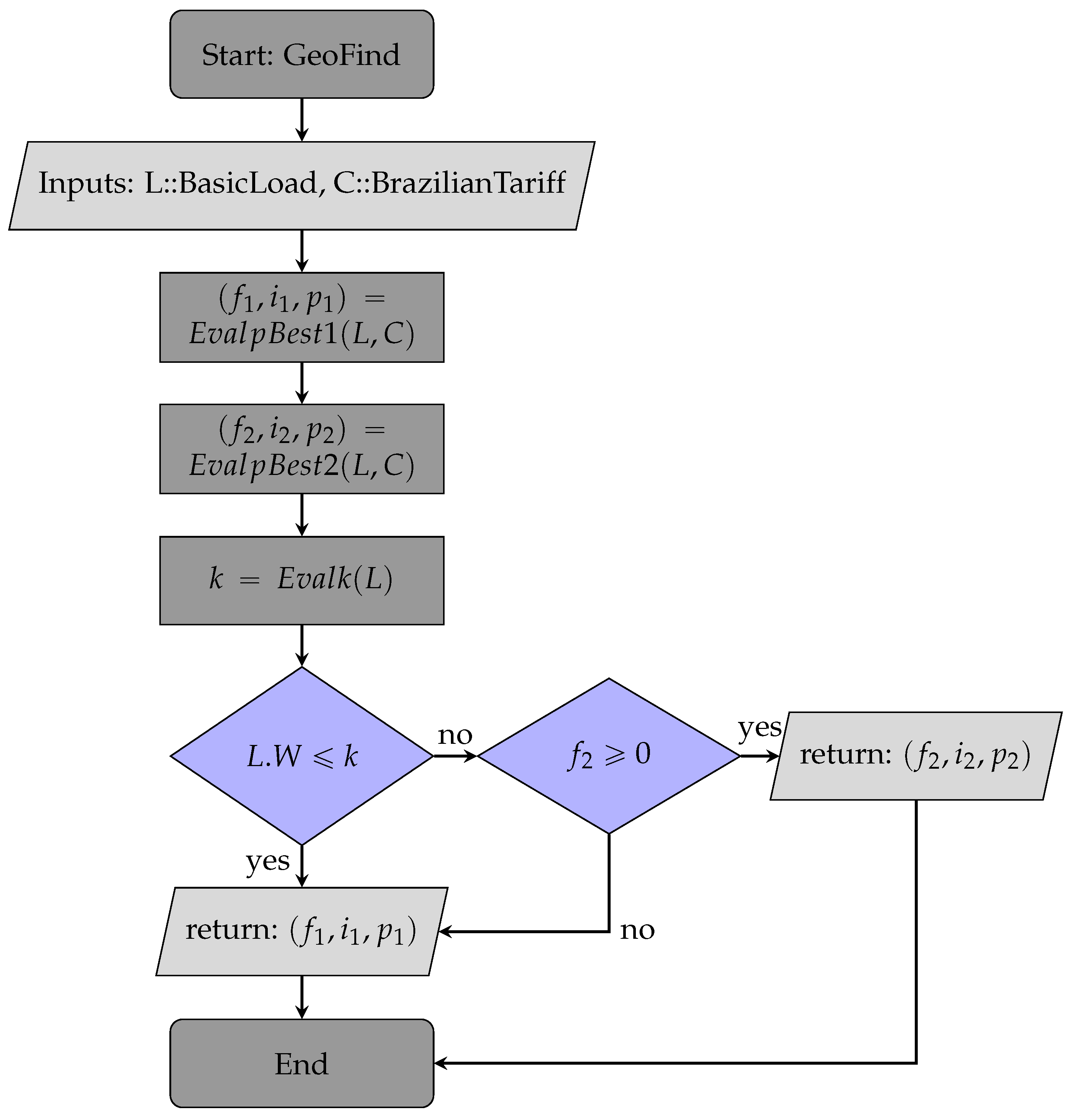
component. The flowchart in
Figure 6 shows the decision process between the two values. Appendix A has link to all code for geometric search process (GeoFind for short).
6.1. Analysis of a Load Fully into off-Peak Post
As stated before, the methodology previous discussed is applicable only if the load has it expected start time inside the interval composed by the intermediate and peak posts. If a load is scheduled by a user fully into off-peak post, no movement should be made with it, as it is already with maximum comfort and lower possible cost.
6.2. Analysis Over Defective Geometric Locus
Due to restrictions caused by the release or deadline instants, some loads may have not fully capability of moving through their geometric locus as defined previously, so it could be considered defective. Lets take an example of a load whose data could be read in
Table 4 and its geometric locus seen in
Figure 7. Note there is no intersection between the geometric locus and the lower cost region. In that specific case we should look at the edges of the possible start times, to find the schedule position with larger component
, and to the expected schedule time. Than evaluate the ratio between cost and comfort for this three instants, as showed in Equation (
28).
The best ratio result between comfort and cost should be returned as solution in this case. A short implementation from statements of this and previous subsection are shown in Algorithm 1.
|
Algorithm 1: Best_Geofind Algorithm |
Require:
ifthen return L.e
end if
if and then return t
end if
return
|
6.3. Analysis of Power Demand Response
So far all analysis that has been made had focused in only one load. As loads could be considered independent, a feasible solution for an array of loads would be iterate the geometric search through a loop and return all schedule instants by recomposing time after find the points in tariff space. One side effect of this solution is that we can not yet add any constraint about demand peaks or maximum power over time.
To cover this issue, a few hypothesis has been formulated and two of them tested through simulation. Both use hierarchical algorithm in combination with output results of geometric search to try speed up their execution and reduce memory use. The first tryout consists in initialize hierarchical algorithm with instant values evaluated with geometric search.
The second approach iterate through the scheduled loads and locate the ones whose summed power exceed demand restriction. After locating the loads that are causing the insurge peak, they are cut from original problem set and passed as parameter to hierarchical algorithm that will try reschedule then within 95% or 90% of the original constraint. This reduction is needed to avoid another demand peaks through reinserting the loads into full set. Then, we check up if all loads fit into demand constraint. In negative case, another cut is made.
Once all loads fit, the iterations end. This last methodology has been named hybrid algorithm. A short version of this method could be seen in Algorithm 2 and its full codification in Julia language can be found in link at Appendix A. Functions that iterates through a set of loads receive the
Vector suffix. As presented in 1 Best_Geofind function combines Geometric search with statements in sub
Section 6.1 and
Section 6.2.
|
Algorithm 2:Hybrid Algorithm |
Require:
Require:▹ default value 0.95
Require:▹ default value 5
while true do ▹ return loads and its indexes if or count ≥ maxIterations then return t end if tcut ← JuMP_MOA_Vector(Hcut; demand=true, demandScale) for i in eachindex(B) do end for count++ end while |
7. Simulations and Results
In Brazil, ANEEL resolution define that there is no charging at residential consumers about demand, only ones in A group has this kind of bill [
12]. That way the methodology presented in this topic would be enough for our local situation. Nevertheless, as vastly discussed before, is a global concern and should be take into account.
As mentioned before, the first simulation scenario is related to a reference house with 11 controllable loads.
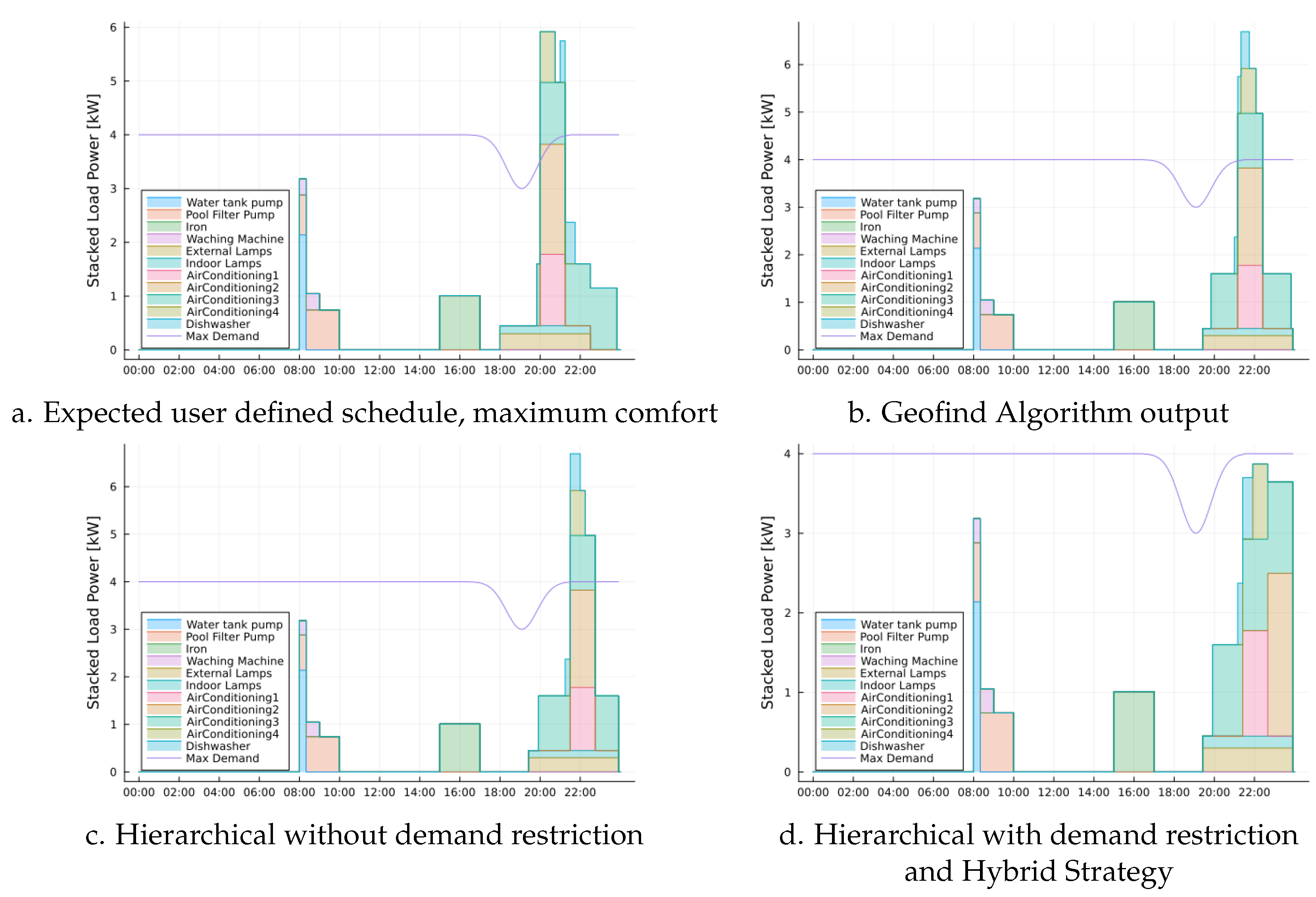
Figure 8 illustrates the scheduling results in a cumulative or stacked load power. The
Figure 8(a) represents the house inhabitants preferences.
Figure 8(b) and (c) show the geometric search and hierarchical results, both without demand constraint. At last,
Figure 8(d) represents the schedule with demand constraint. The three least methodologies returned the same quantitative result videlicet: Hierarchical with DR, Hierarchical with DR constraint and initialized with geometric search results and the hybrid strategy. Although, only the two purely based Hierarchical algorithm were expected to return the same qualitative results. This result has occurred due to small quantity of loads in this simulation set and because a significantly amount of then were selected to run into Hierarchical. In quantitative analysis, only hybrid strategy has achieved better benchmarks as hypothetically expected.
In
Table 5 the values of comfort and normalized cost for reference house scenario can be read. Note that best comfort values are realized by the methodology presented in this paper.
The results of geometric search could be equal to hierarchical by adjusting the code to return the next inner point in lower cost region, and not the first one. All results achieved are compatible with cited previous works.
During experiments with first scenario data, it has been noted that the output results of geometric search were a way faster than ones obtained by linear programming tool. Furthermore, less memory has also been allocated while evaluation. To stand this result and verify its impact with larger sets of data, we proposed to generate eight sets of data with increasing size in scale, as told in section 2. Each set of data has been submitted to five different scheduling procedures:
Geometric Search;
Multi-objective Hierarchical without demand constraint;
Multi-objective Hierarchical with demand constraint;
Multi-objective Hierarchical with demand constraint and initialized with Geofind solution;
Hybrid algorithm.
The five scheduling results and the random generated expected time schedule can be seen in details for each data set in link at Appendix A.
All benchmarks results presented and discussed here has been run for at least 25 times, to avoid long execution simulations, but most data has been collected through 100 or more executions under same conditions and computer (Intel Core i5 2410M 2.3GHz with 6GB of DDR3 Memory using ZorinOS and Julia 1.8.5) an iteration number that has been considered enough due to all results evaluated in each procedure always provided same solution. All benchmarks outputs, including detailed histograms, can be found in link provided at Appendix A.
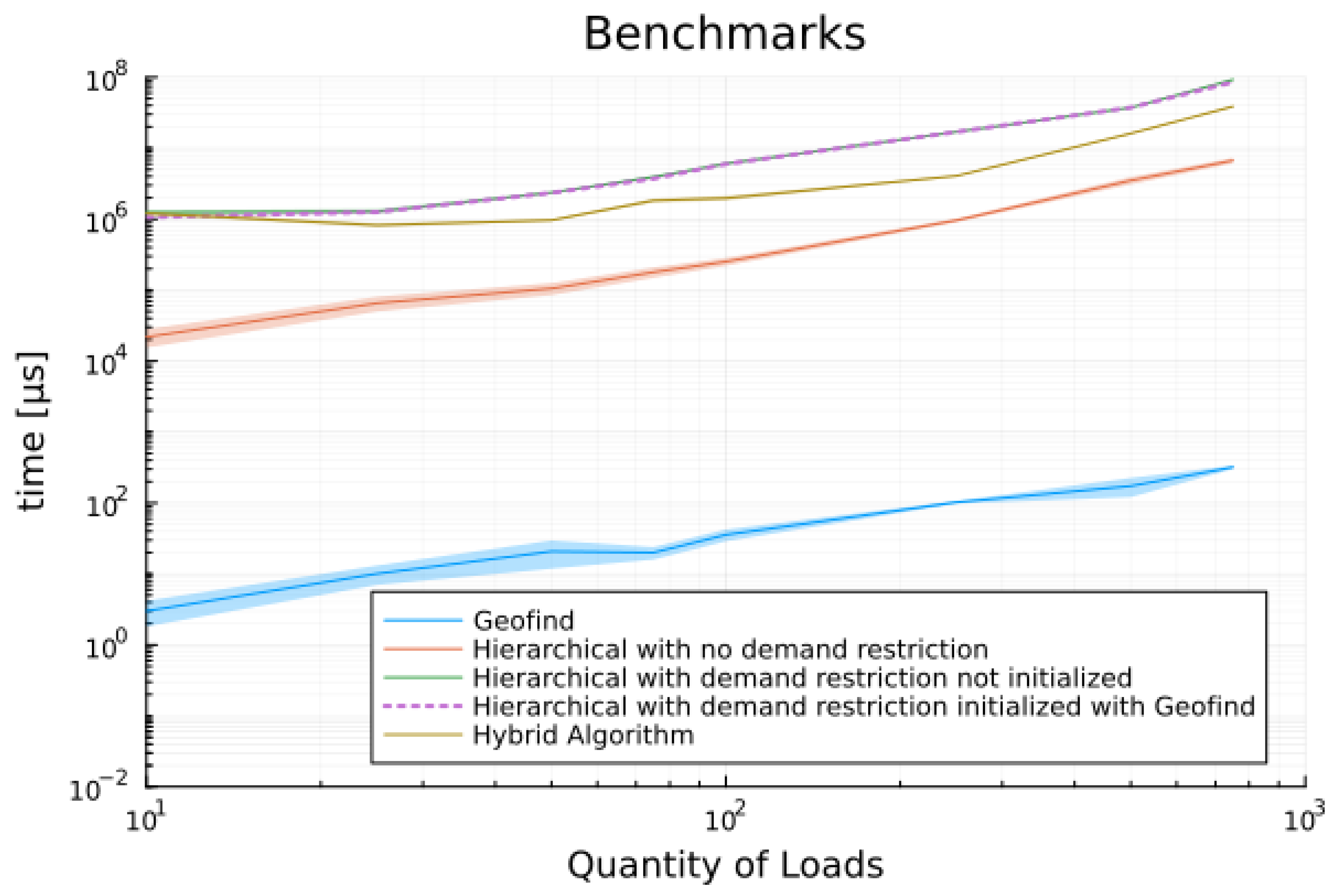
Data in
Table 6 shows the mean execution time for all random scenarios. Note that geometric search stays at microseconds while other solutions grow large reaching tens of seconds to display the results. Also note that the times collected for Hierarchical algorithm initialized with the output of geometric search is just slight better then its non-initialized version. However, hybrid proposed methodology has improved about
in comparison to hierarchical results. This same discussion could be applied to memory estimate data presented in
Table 7.
Figure 9 illustrates the benchmark results for time.
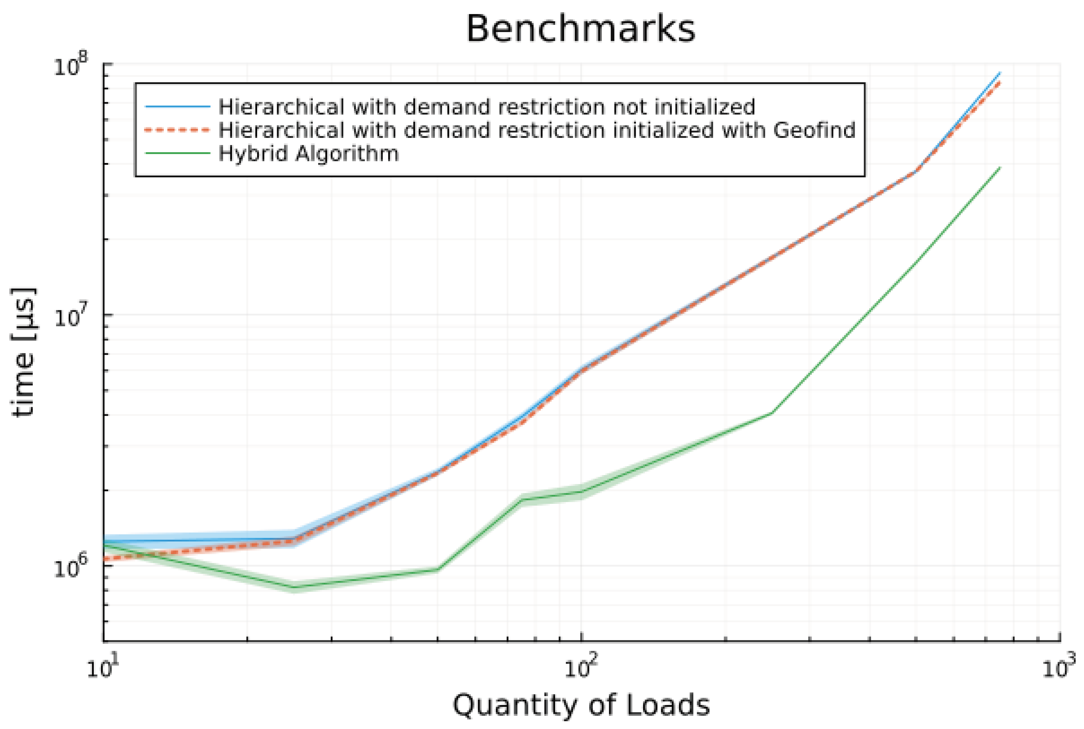
Figure 10 shows a cut of the previous one to allow the reader see the difference between two executions of hierarchical algorithm and how better the hybrid solution has been.
The next data presented here are the values for comfort (
Table 8) and normalized cost (
Table 9) evaluated for each load set applying all five scheduling methodologies. As occurred in scenario one, the geometric search has a better result in comfort metric than hierarchical algorithm without DR restriction while achieve the goal to lower the energy cost due to constant tariff. The Hybrid algorithm has also achieved better comfort metrics when compared to Hierarchical results while all three algorithms have processed the DR constraint. For a better view of this results, the reader can see the graphics available in link at Appendix A.
To finish our discussion about the results,
Table 10 presents the data set that has been processed by hierarchical algorithm inside hybrid solution and how many iterations it has executed to compliance with demand constraint.
Excluding the results presented at first line of
Table 10, after the scheduling has been processed by geometric search an amount that varies from a third to a half of the loads in random datasets are agglutinated, causing a demand peak. So, through hybrid methodology we have been able to reduce the amount of data processed by the LP tool, what explain the related improvement. Also note that hybrid methodology have done few search iterations, which demonstrates the efficiency of this method too. In the first case, the amount of loads causing demand peak where very close to total quantity (9 out 10). That way, the search processing and running hierarchical algorithm with reinforced constraint due to scale reduction results were similar to the original linear programming tool with 10 loads, so it is a valid effort.
8. Conclusions
Achieving simultaneous objectives of energy efficiency and comfort is not an easy task, as it represent an intricate trade-off between the need to reduce energy bill and stand for user preferences. The proposed solution performs fast optimization in a SH scenario whose ToU takes into account three tariff posts: off peak, intermediate and peak. That stated, the main goal of this work was to present a new methodology for scheduling of home electric loads minimizing cost but without sacrifice inhabitants comfort rate.
To reach the main goal, including the fact that it has been show that a set of appliances can be modeled as an independent set, a novel methodology based on the definitions of tariff space, decomposition of time axis into multiple independent dimensions and geometric locus of a load that models the behavior of an appliance as it moves through tariff space or time itself has been presented in this paper. Through explanation, examples of each definition has been given and explored step by step.
The benchmark results for processing time during result evaluation and memory usage presented in
Table 6 and
Table 7 for the load scheduling problem without demand restriction are an order of magnitude ten thousand times better than the solution evaluated by LP multi-objective counterpart.
The output results for comfort and cost presented in
Table 8 and
Table 9 have shown the reliability of proposed methodologies as outputs for all methods are quite similar. Better results for comfort metric are expected for the new scheduler proposed in this work, as it concept methodology gives the shortest distance of movement in time necessary to reduce the energy bill. To achieve a fair goal, the importance factor
of all loads and in all simulations has been set to one.
The presented methodology for scheduling appliances in a SH environment fits legal regulations in Brazilian energy market, and is capable to solve large instances of this problem in less than a few milliseconds. Also, the reduction in memory usage by geometric search has a true potential to physical implementation of this solution in low cost embedded systems in a way that could improve HEMS in a nearest future and help popularize this kind of equipment.
Besides optimization, it is also important achieve energy bill savings constrained by flattening demand as this contributes to reduce investments of the energy suppliers through distribution network, decreasing the constant need to expand the system to maintain the availability of ever-increasing energy consumption [
9]. Although current state of geometric search is not able yet to directly relate with demand restrictions by itself, the present work has also tested two methodologies to enhance the geometric search methodology so it could also comply with demand response restriction problems. The proposed hybrid algorithm achieved superior benchmark results than its linear programming counter part, achieving for larger loads set improvements of at least 40% . Although, better ways to include demand constraints should be also included into future works. Some other hypothesis using Game Theory [
53] and Topological Algebra are currently in study.
Time itself is a substantially complex subject and this work may started to open an window which will allow us to explore even further its properties. The decomposition of time into a geometric space is a new methodology that is far away to reach its full potential. Future research should include extrapolation of tariff space for hour based tariffs or even continuous ones. The works proposed by [
59,
60] seems to be a key path to continue this discussion.
Author Contributions
Conceptualization, Luis Rodolfo Rebouças Coutinho; Formal analysis, Luis Rodolfo Rebouças Coutinho; Methodology, Luis Rodolfo Rebouças Coutinho; Project administration, Giovanni Barroso; Supervision, Giovanni Barroso and Bruno Prata; Validation, Luis Rodolfo Rebouças Coutinho; Writing – original draft, Luis Rodolfo Rebouças Coutinho; Writing – review and editing, Giovanni Barroso and Bruno Prata. All authors have read and agreed to the published version of the manuscript.
Funding
This work was supported by the Brazilian National Council for Scientific and Technological Development (Conselho Nacional de Desenvolvimento Científico e Tecnológico), through grants 309755/2021-2, and 407151/2021-4; and the Brazilian Coordination for the Improvement of Higher Education Personnel (Coordenação de Aperfeiçoamento de Pessoal de Nível Superior), Financial Code No. 001.
Abbreviations
The following abbreviations are used in this manuscript:
Appendix A. GitHub Project Page
The GitHub link bellow has all extra information needed to follow all procedures in this papper.
References
- Sanghvi, A.P. Flexible strategies for load/demand management using dynamic pricing. IEEE Trans. Power Syst. 1989, 4. [Google Scholar] [CrossRef]
- Ipakchi, A.; Albuyeh, F. Grid of the future. IEEE Power Energy Mag. 2009, 7. [Google Scholar] [CrossRef]
- Clement-Nyns, K.; Haesen, E.; Driesen, J. The impact of charging plug-in hybrid electric vehicles on a residential distribution grid. IEEE Trans. Power Syst. 2009, 25. [Google Scholar] [CrossRef]
- Sortomme, E.; El-Sharkawi, M.A. Optimal charging strategies for unidirectional vehicle-to-grid. IEEE Trans. Smart Grid 2010, 2. [Google Scholar] [CrossRef]
- 110th Congress (2007). H.R. 6 (110th), 2007.
- Bleviss, D.L. Transportation is critical to reducing greenhouse gas emissions in the United States. Wiley Interdisciplinary Reviews: Energy and Environment 2021, 10. [Google Scholar] [CrossRef]
- Gellings, C.W.; Samotyj, M. Smart Grid as advanced technology enabler of demand response. Energy Efficiency 2013, 6, 685–694. [Google Scholar] [CrossRef]
- Hu, Z. Review of dynamic pricing programs in the US and Europe: Status quo and policy recommendations. Renew. Sust. Energ. Rev. 2015, 42. [Google Scholar] [CrossRef]
- de Albuquerque, P.U.B. Estudo e Desenvolvimento de Abordagens Multiobjetivo Baseadas em Programação Linear e em Metaheurísticas para Otimização do Custo com Energia Elétrica e do Conforto do Usuário. PhD thesis, Universidade Federal do Ceará, 2018.
- Perera, A.; Kamalaruban, P. Applications of reinforcement learning in energy systems. Renew. Sust. Energ. Rev. 2021, 137. [Google Scholar] [CrossRef]
- dos Santos, S.A.B.; Soares, J.M.; Barroso, G.C.; de Athayde Prata, B. Demand response application in industrial scenarios: A systematic mapping of practical implementation. Expert Systems with Applications 2023, 215. Export Date: 28 September 2023; Cited By: 1. [Google Scholar] [CrossRef]
- ANEEL. RESOLUÇÃO NORMATIVA ANEEL Nº 1.000, DE 7 DE DEZEMBRO DE 2021. 2021.
- ANEEL. Base de Dados das Tarifas das Distribuidoras de Energia Elétrica. 2023.
- ENEL-CE. Tarifa de fornecimento - Baixa tensão. 2023.
- Kim, T.T.; Poor, H.V. Scheduling power consumption with price uncertainty. IEEE Trans. Smart Grid 2011, 2. [Google Scholar] [CrossRef]
- Giorgio, A.; Pimpinella, L. An event driven smart home controller enabling consumer economic saving and automated demand-side management. Applied Energy 2012, 96. [Google Scholar] [CrossRef]
- Chen, X.; Wei, T.; Hu, S. Uncertainty-aware household appliance scheduling considering dynamic electricity pricing in smart home. IEEE Trans. Smart Grid 2013, 4. [Google Scholar] [CrossRef]
- Qayyum, F.A. Appliance Scheduling Optimization in Smart Home Networks. IEEE Access 2015, 3. [Google Scholar] [CrossRef]
- Wang, C.; Zhou, Y.; Jiao, B.; Wang, Y.; Liu, W.; Wang, D. Robust optimization for load scheduling of a smart home with photovoltaic system. Energy Convers. Manag. 2015, 102. [Google Scholar] [CrossRef]
- Huang, Y.; Wang, L.; Guo, W.; Kang, Q.; Wu, Q. Chance constrained optimization in a home energy management system. IEEE Trans. Smart Grid. 2016, 9. [Google Scholar] [CrossRef]
- Rahmani-Andebili, M. Scheduling deferrable appliances and energy resources of a smart home applying multi-time scale stochastic model predictive control. Sustain. Cities Soc. 2017, 32. [Google Scholar] [CrossRef]
- Farrokhifar, M. Real-time based approach for intelligent building energy management using dynamic price policies. Sustain. Cities Soc. 2018, 37. [Google Scholar] [CrossRef]
- Lu, Q.; Zhang, Z.; Lü, S. Home energy management in smart households: Optimal appliance scheduling model with photovoltaic energy storage system. Energy Reports 2020, 6, 2450–2462. [Google Scholar] [CrossRef]
- Luo, F.; Kong, W.; Ranzi, G.; Dong, Z.Y. Optimal home energy management system with demand charge tariff and appliance operational dependencies. IEEE Transactions on Smart Grid 2020, 11, 4–14. [Google Scholar] [CrossRef]
- Costa, J.R.D.; Barroso, G.C.; Souza, D.A.D.; Batista, J.G.; Junior, A.B.D.S.; Rios, C.; Vasconcelos, F.; Júnior, J.; Bezerra, I.D.S.; Lima, A.F.D.; Santana, K.A.D.; Júnior, J.R.D.O. An Improved Optimization Function to Integrate the User’s Comfort Perception into a Smart Home Controller Based on Particle Swarm Optimization and Fuzzy Logic. Sensors 2023, 23. [Google Scholar] [CrossRef]
- Mohsenzadeh, A.; Shariatkhah, M.H.; Haghifam, M.R. Applying fuzzy techniques to model customer comfort in a smart home control system. 22nd International Conference and Exhibition on Electricity Distribution (CIRED 2013), 2013, pp. 1–4. [CrossRef]
- Chekired, F.; Mahrane, A.; Samara, Z.; Chikh, M.; Guenounou, A.; Meflah, A. Fuzzy logic energy management for a photovoltaic solar home. Energy Procedia 2017, 134. [Google Scholar] [CrossRef]
- Filho, P.B.; Albuquerque, P.; Prata, B.; Barroso, G. A smart home controller using an integer programming approach for the optimization of consumer economic saving and comfort. Proceedings of the XII SBAI Simpósio Brasileiro de Automação Inteligente (Brazilian Symposium in Intelligent Automation), Natal-RN, Brazil. 2015; 25. [Google Scholar]
- Albuquerque, P.U.B.; de A Ohi, D.K.; Pereira, N.S.; de A Prata, B.; Barroso, G.C. Proposed Architecture for Energy Efficiency and Comfort Optimization in Smart Homes. Journal of Control, Automation and Electrical Systems 2018, 29, 718–730. [Google Scholar] [CrossRef]
- Ma, K.; Yao, T.; Yang, J.; Guan, X. Residential power scheduling for demand response in smart grid. International Journal of Electrical Power & Energy Systems 2016, 78, 320–325. [Google Scholar] [CrossRef]
- Ogunjuyigbe, A.S.O.; Ayodele, T.R.; Akinola, O.A. User satisfaction-induced demand side load management in residential buildings with user budget constraint. Applied Energy 2017, 187, 352–366. [Google Scholar] [CrossRef]
- Manzoor, A.; Javaid, N.; Ullah, I.; Abdul, W.; Almogren, A.; Alamri, A. An Intelligent Hybrid Heuristic Scheme for Smart Metering based Demand Side Management in Smart Homes. Energies 2017, 10. [Google Scholar] [CrossRef]
- Chen, Z.; Chen, Y.; He, R.; Liu, J.; Gao, M.; Zhang, L. Multi-objective residential load scheduling approach for demand response in smart grid. Sustain Cities Soc 2022, 76. [Google Scholar] [CrossRef]
- Lin, Y.H.; Hu, Y.C. Residential Consumer-Centric Demand-Side Management Based on Energy Disaggregation-Piloting Constrained Swarm Intelligence: Towards Edge Computing. Sensors 2018, 18. [Google Scholar] [CrossRef]
- dos Santos, S.A.B. Utilização da meta-heurística PSO para otimização multiobjetivo de um SMART HOME CONTROLLER. Master’s thesis, Universidade Federal do Ceará, 2019.
- Gazafroudi, A.S.; Shafie-khah, M.; Heydarian-Forushani, E.; Hajizadeh, A.; Heidari, A.; Corchado, J.M.; Catalão, J.P. Two-stage stochastic model for the price-based domestic energy management problem. International Journal of Electrical Power and Energy Systems 2019, 112, 404–416. [Google Scholar] [CrossRef]
- Akbari-Dibavar, A. Smart home energy management using hybrid robust-stochastic optimization. Comput. Ind. Eng. 2020, 143. [Google Scholar] [CrossRef]
- Zeynali, S.; Rostami, N.; Ahmadian, A.; Elkamel, A. Two-stage stochastic home energy management strategy considering electric vehicle and battery energy storage system: An ANN-based scenario generation methodology. Sustainable Energy Technologies and Assessments 2020, 39, 100722. [Google Scholar] [CrossRef]
- Ali, S. Demand response program for efficient demand-side management in smart grid considering renewable energy sources. IEEE Access 2022, 10. [Google Scholar] [CrossRef]
- García, O.; Prieto, J.; Alonso, R.S.; Corchado, J.M. A framework to improve energy efficient behaviour at home through activity and context monitoring. Sensors 2017, 17. [Google Scholar] [CrossRef]
- González-Briones, A.; Prieto, J.; Prieta, F.; Herrera-Viedma, E.; Corchado, J.M. Energy optimization using a case-based reasoning strategy. Sensors 2018, 18. [Google Scholar] [CrossRef]
- Schirmer, P.A.; Mporas, I. Non-intrusive load monitoring: a review. IEEE Trans Smart Grid 2023, 14. [Google Scholar] [CrossRef]
- Rajasekhar, B.; Pindoriya, N.; Tushar, W.; Yuen, C. Collaborative Energy Management for a Residential Community: A Non-Cooperative and Evolutionary Approach. IEEE Transactions on Emerging Topics in Computational Intelligence 2019, 3, 177–192. [Google Scholar] [CrossRef]
- Çimen, H.; Bazmohammadi, N.; Lashab, A.; Terriche, Y.; Vasquez, J.C.; Guerrero, J.M. An online energy management system for AC/DC residential microgrids supported by non-intrusive load monitoring. Appl Energy 2022, 307. [Google Scholar] [CrossRef]
- Mansouri, S.A.; Ahmarinejad, A.; Nematbakhsh, E.; Javadi, M.S.; Nezhad, A.E.; Catalão, J.P. A sustainable framework for multi-microgrids energy management in automated distribution network by considering smart homes and high penetration of renewable energy resources. Energy 2022, 245. [Google Scholar] [CrossRef]
- O’Grady, T.; Chong, H.Y.; Morrison, G.M. A systematic review and meta-analysis of building automation systems, 2021. [CrossRef]
- ASHRAE, A.H. Fundamentals, SI ed. American Society of Heating, Refrigerating and Air-Conditioning Engineers, Atlanta, GA 2017, 2017. [Google Scholar]
- Aliabadi, F.E.; Agbossou, K.; Kelouwani, S.; Henao, N.; Hosseini, S.S. Coordination of smart home energy management systems in neighborhood areas: A systematic review. IEEE Access 2021, 9, 36417–36443. [Google Scholar] [CrossRef]
- Merabet, G.H.; Essaaidi, M.; Haddou, M.B.; Qolomany, B.; Qadir, J.; Anan, M.; Al-Fuqaha, A.; Abid, M.R.; Benhaddou, D. Intelligent building control systems for thermal comfort and energy-efficiency: A systematic review of artificial intelligence-assisted techniques. 2021. [Google Scholar] [CrossRef]
- Balakrishnan, R.; Geetha, V. Review on home energy management system. Materials Today: Proceedings, 2021. [Google Scholar] [CrossRef]
- Mekuria, D.N.; Sernani, P.; Falcionelli, N.; Dragoni, A.F. Smart home reasoning systems: a systematic literature review. Journal of Ambient Intelligence and Humanized Computing 2021, 12, 4485–4502. [Google Scholar] [CrossRef]
- Mischos, S.; Dalagdi, E.; Vrakas, D. Intelligent energy management systems: a review. Artificial Intelligence Review 2023, 56, 11635–11674. [Google Scholar] [CrossRef]
- Coutinho, L.R.R. MÉTODO DE ORDENAÇÃO DE EVENTOS PARA SISTEMAS EMBARCADOS MULTITAREFA COM MÚLTIPLOS NÍVEIS CRÍTICOS. Master’s thesis, Universidade Estadual do Ceará, 2013.
- Lubin, M.; Dowson, O.; Dias Garcia, J.; Huchette, J.; Legat, B.; Vielma, J.P. JuMP 1.0: Recent improvements to a modeling language for mathematical optimization. Mathematical Programming Computation 2023. [Google Scholar] [CrossRef]
- Bezanson, J.; Edelman, A.; Karpinski, S.; Shah, V.B. Julia: A fresh approach to numerical computing. SIAM Review 2017, 59, 65–98. [Google Scholar] [CrossRef]
- Downson, O.; et al. MultiObjectiveAlgorithms.jl (MOA) is a collection of algorithms for multi-objective optimization., 2023. MultiObjectiveAlgorithms.jl is licensed under the MPL 2.0 License.
- Lubin, M.; Dunning, I. Computing in Operations Research Using Julia. INFORMS Journal on Computing 2015, 27, 238–248. [Google Scholar] [CrossRef]
- Dunning, I.; Huchette, J.; Lubin, M. JuMP: A Modeling Language for Mathematical Optimization. SIAM Review 2017, 59, 295–320. [Google Scholar] [CrossRef]
- Hausmann, J.C.; Knutson, A. Polygon spaces and Grassmannians. arXiv: Differential Geometry 1996. [Google Scholar] [CrossRef]
- Hausmann, J.C.; Knutson, A. The cohomology ring of polygon spaces. Annales de l’institut Fourier 1998, 48, 281–321. [Google Scholar] [CrossRef]
Figure 1.
Load model and timing parameters.
Figure 1.
Load model and timing parameters.
Figure 2.
Multiple stage load to multiple simple loads.
Figure 2.
Multiple stage load to multiple simple loads.
Figure 3.
Three different startup times for a 4 hours load around intermediate and peak post tariffs.
Figure 3.
Three different startup times for a 4 hours load around intermediate and peak post tariffs.
Figure 4.
All startup times for a 1 hour load crossing intermediate and peak post tariffs.
Figure 4.
All startup times for a 1 hour load crossing intermediate and peak post tariffs.
Figure 5.
Example of startup times for a 6 hours load crossing intermediate and peak post tariffs.
Figure 5.
Example of startup times for a 6 hours load crossing intermediate and peak post tariffs.
Figure 6.
Geometric Search Flowchart.
Figure 6.
Geometric Search Flowchart.
Figure 7.
Example of a defective load into tariff space time.
Figure 7.
Example of a defective load into tariff space time.
Figure 8.
Reference House loads user schedule and output results.
Figure 8.
Reference House loads user schedule and output results.
Figure 9.
Benchmarks results for execution time.
Figure 9.
Benchmarks results for execution time.
Figure 10.
Benchmarks results for execution time, only algorithms with demand response constraint.
Figure 10.
Benchmarks results for execution time, only algorithms with demand response constraint.
Table 1.
Comparison between conventional tariff and white tariff over time.
Table 1.
Comparison between conventional tariff and white tariff over time.
| Period |
Tariff |
|
White Tariff |
| |
Post |
(R$/kWh) |
(R$/kWh) |
| 00:00 to 16:30 |
Off-peak |
0.74373 |
0.62124 |
| 16:30 to 17:30 |
Intermediate |
0.74373 |
1.03901 |
| 17:30 to 20:30 |
Peak |
0.74373 |
1.63527 |
| 20:30 to 21:30 |
Intermediate |
0.74373 |
1.03901 |
| 21:30 to 00:00 |
Off-peak |
0.74373 |
0.62124 |
Table 2.
List of symbols that define parameters of a BasicLoad structure in Julia language.
Table 2.
List of symbols that define parameters of a BasicLoad structure in Julia language.
| Id |
Description |
|
release time of the load |
|
expected time of the load |
|
deadline instant of the load |
|
range with all possible start times of the load,
|
|
finishing time of the load,
|
|
discrete step in which a load could move through time, common to all loads in set |
|
width of the load, usually measured in minutes |
|
discrete load width |
|
behavior of the load through time |
|
average power of the load |
|
peak power of the load |
|
relevance of the load,
|
| k |
proportion of discrete time related to 1 hour,
|
Table 3.
Reference loads in an actual residence
Table 3.
Reference loads in an actual residence
| ID |
Load |
Cycles |
|
|
|
Expected |
Release |
Deadline |
|
| |
|
|
|
|
|
Time |
Time |
Time |
|
| 1 |
Water tank pump |
1 |
20 |
2 |
3 |
8h |
7h |
17h |
1.0 |
| 2 |
Pool filter pump |
1 |
120 |
0.75 |
1.5 |
8h |
7h |
17h |
1.0 |
| 3 |
Iron |
1 |
120 |
1 |
1.2 |
16h |
14h |
17h |
1.0 |
| 4 |
Washing machine |
8 |
10 10 4 6 2 2 2 7 |
0.13 0.51 0.30, 0.26 0.15 ⋯ 0.22 |
0.70 0.50 0.30 0.26 0.15 ⋯ 0.30 |
8h |
7h |
17h |
1.0 |
| 5 |
External lamps |
1 |
270 |
0.3 |
0.3 |
18h |
17h |
24h |
1.0 |
| 6 |
Indoor lamps |
1 |
270 |
0.15 |
0.3 |
18h |
17h |
23h |
1.0 |
| 7 |
Air Conditioning 1 |
14 |
[10 5 5 ⋯ 5] |
[1.3 ⋯ 1.3] |
[1.7 1.3 ⋯ 1.3] |
16h |
15h |
24h |
1.0 |
| 8 |
Air Conditioning 2 |
7 |
[30 20 5 ⋯ 5] |
[2 ⋯ 2] |
[2.1 ⋯ 2.1] |
20h |
17h |
24h |
1.0 |
| 9 |
Air Conditioning 3 |
1 |
240 |
1.1 |
1.2 |
20h |
17h |
24h |
1.0 |
| 10 |
Air Conditioning 4 |
7 |
[10 10 5⋯ 5] |
[0,9 ⋯ 0.9] |
[1,1 ⋯ 1.1] |
20h |
17h |
24h |
1.0 |
| 11 |
Dishwasher |
5 |
5, 10, 15, 5, 10 |
0.03, 1.76, 0.03, 1.76, 0.03 |
0.03, 1.76, 0.03, 1.76, 0.03 |
21h |
18h |
22h |
1.0 |
Table 4.
Example of a load with defective geometric locus.
Table 4.
Example of a load with defective geometric locus.
| L.r |
L.e |
L.d |
|
L.W |
| 16h |
18h |
23h |
5min |
3h |
Table 5.
Mean comfort and cost for reference house appliances.
Table 5.
Mean comfort and cost for reference house appliances.
| Algorithm |
Comfort |
Cost |
| Expected user time |
1.000 |
1.311 |
| Geofind |
0.873 |
1.021 |
| Hierarchical without DR |
0.845 |
0.965 |
| Hierarchical with DR |
0.813 |
0.974 |
| Hierarchical with DRa
|
0.813 |
0.974 |
| Hybrid algorithm |
0.813 |
0.974 |
Table 6.
Mean execution time benchmarks for random loads scenario.
Table 6.
Mean execution time benchmarks for random loads scenario.
| Random |
Geofind |
Hierarchical |
Hierarchical |
Hierarchical |
Hybrid |
| Loads |
without DR |
without DR |
with DR |
with DR a
|
algorithm |
| 10 |
3.005 s |
0.022 s |
1.249 s |
1.066 s |
1.208 s |
| 25 |
10.074 s |
0.065 s |
1.285 s |
1.256 s |
0.822 s |
| 50 |
20.748 s |
0.105 s |
2.370 s |
2.343 s |
0.966 s |
| 75 |
19.975 s |
0.179 s |
3.933 s |
3.715 s |
1.829 s |
| 100 |
35.647 s |
0.252 s |
6.055 s |
5.968 s |
1.975 s |
| 250 |
102.471 s |
0.962 s |
16.864 s |
16.919 s |
4.061 s |
| 500 |
173.276 s |
3.509 s |
37.316 s |
37.328 s |
16.124 s |
| 750 |
319.320 s |
6.699 s |
92.339 s |
84.897 s |
38.664 s |
Table 7.
Memory estimate benchmarks for random loads scenario.
Table 7.
Memory estimate benchmarks for random loads scenario.
| Random |
Geofind |
Hierarchical |
Hierarchical |
Hierarchical |
Hybrid |
| Loads |
without DR |
without DR |
with DR |
with DR a
|
algorithm |
| 10 |
1.17 KiB |
5.84 MiB |
37.84 MiB |
37.84 MiB |
36.53 MiB |
| 25 |
3.66 KiB |
19.09 MiB |
92.67 MiB |
92.64 MiB |
60.82 MiB |
| 50 |
5.45 KiB |
40.51 MiB |
180.14 MiB |
180.07 MiB |
82.99 MiB |
| 75 |
7.50 KiB |
72.37 MiB |
273.62 MiB |
273.53 MiB |
153.42 MiB |
| 100 |
15.59 KiB |
123.39 MiB |
421.92 MiB |
421.79 MiB |
161.99 MiB |
| 250 |
31.16 KiB |
508.57 MiB |
1.21 GiB |
1.21 GiB |
303.17 MiB |
| 500 |
68.56 KiB |
1.72 GiB |
3.13 GiB |
3.13 GiB |
1.22 GiB |
| 750 |
97.38 KiB |
3.67 GiB |
5.93 GiB |
5.93 GiB |
2.67 GiB |
Table 8.
Mean normalized comfort for random loads scenario.
Table 8.
Mean normalized comfort for random loads scenario.
| Random |
Geofind |
Hierarchical |
Hierarchical |
Hierarchical |
Hybrid |
| Loads |
without DR |
without DR |
with DR |
with DR a
|
algorithm |
| 10 |
0.976 |
0.974 |
0.887 |
0.887 |
0.887 |
| 25 |
0.963 |
0.948 |
0.945 |
0.945 |
0.957 |
| 50 |
0.942 |
0.942 |
0.941 |
0.941 |
0.935 |
| 75 |
0.965 |
0.964 |
0.962 |
0.962 |
0.963 |
| 100 |
0.941 |
0.935 |
0.934 |
0.9341 |
0.945 |
| 250 |
0.968 |
0.959 |
0.958 |
0.958 |
0.967 |
| 500 |
0.947 |
0.934 |
0.937 |
0.937 |
0.944 |
| 750 |
0.954 |
0.940 |
0.941 |
0.941 |
0.946 |
Table 9.
Mean normalized cost for random loads scenario.
Table 9.
Mean normalized cost for random loads scenario.
| Random |
Geofind |
Hierarchical |
Hierarchical |
Hierarchical |
Hybrid |
| Loads |
without DR |
without DR |
with DR |
with DRa
|
algorithm |
| 10 |
0.871 |
0.828 |
0.843 |
0.843 |
0.843 |
| 25 |
0.923 |
0.893 |
0.893 |
0.893 |
0.914 |
| 50 |
0.859 |
0.833 |
0.839 |
0.839 |
0.839 |
| 75 |
0.873 |
0.852 |
0.852 |
0.852 |
0.873 |
| 100 |
0.910 |
0.863 |
0.863 |
0.863 |
0.907 |
| 250 |
0.881 |
0.847 |
0.847 |
0.847 |
0.881 |
| 500 |
0.897 |
0.854 |
0.858 |
0.858 |
0.885 |
| 750 |
0.885 |
0.846 |
0.848 |
0.848 |
0.862 |
Table 10.
Hybrid algorithm running parameters for random loads scenario.
Table 10.
Hybrid algorithm running parameters for random loads scenario.
| Random Loads |
Loads causing demand peak |
Search iterations |
| 10 |
9 |
1 |
| 25 |
14 |
1 |
| 50 |
22 |
1 |
| 75 |
19 |
2 |
| 100 |
41 |
1 |
| 250 |
75 |
1 |
| 500 |
123 |
2 |
| 750 |
217 |
2 |
|
Disclaimer/Publisher’s Note: The statements, opinions and data contained in all publications are solely those of the individual author(s) and contributor(s) and not of MDPI and/or the editor(s). MDPI and/or the editor(s) disclaim responsibility for any injury to people or property resulting from any ideas, methods, instructions or products referred to in the content. |
© 2024 by the authors. Licensee MDPI, Basel, Switzerland. This article is an open access article distributed under the terms and conditions of the Creative Commons Attribution (CC BY) license (http://creativecommons.org/licenses/by/4.0/).
