Submitted:
19 February 2024
Posted:
20 February 2024
You are already at the latest version
Abstract
Keywords:
Introduction
Materials and Methods
1. Material
2. Experiment design
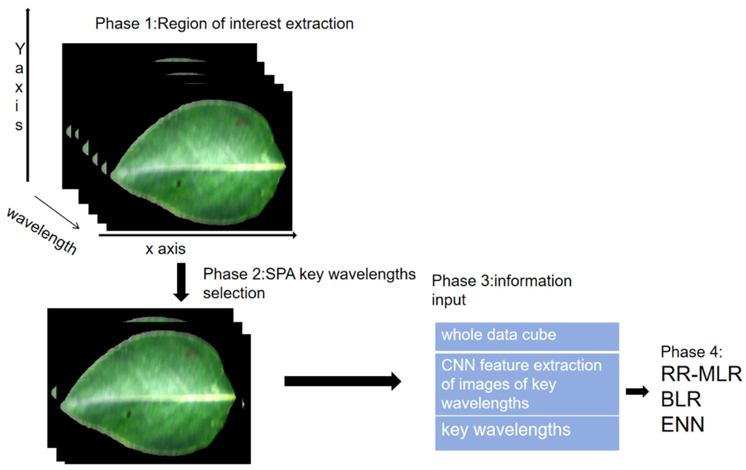
2.1. Hyperspectral image acquisition
2.2. Image acquisition and image correction
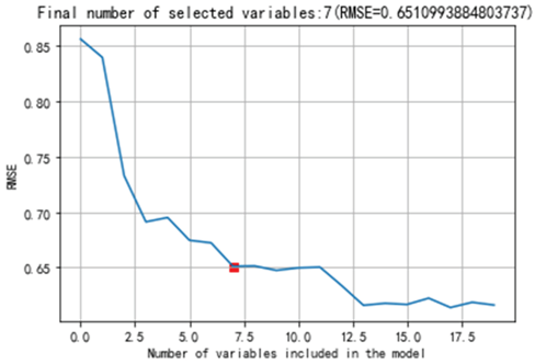
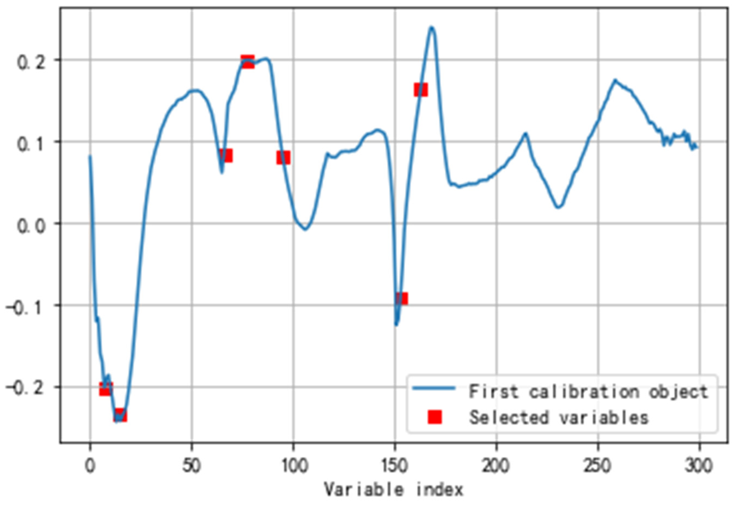
2.3. Feature wavelength selection
3. Machine learning methods
3.1. Convolutional neural network (CNN) feature extraction
3.2. Baseline model
3.2.1. Data Classification for Multiple Linear Regression Based on Ridge Regression
3.2.2. Bayesian linear regression
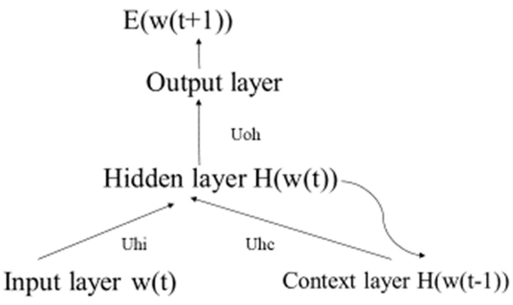
3.2.3. Elman Neural Network
4. Performance metrics
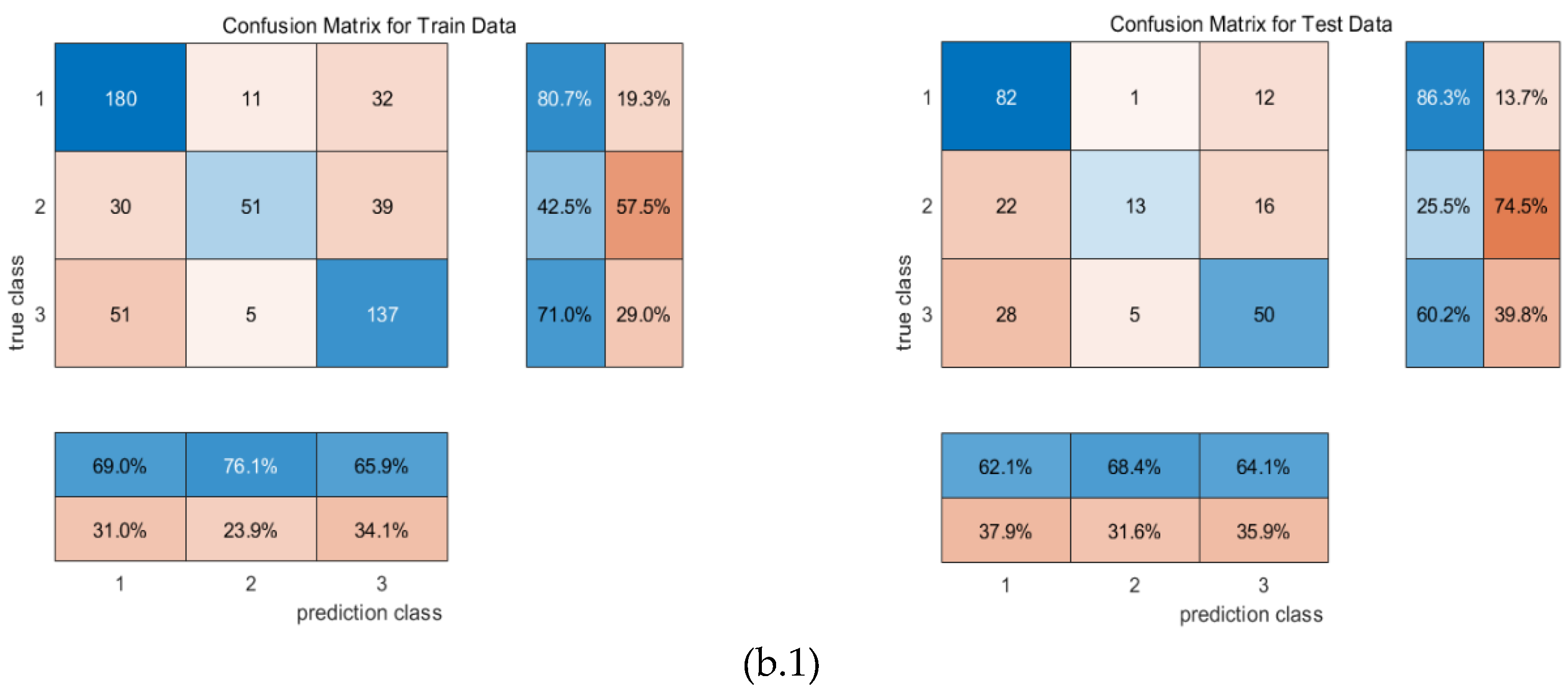
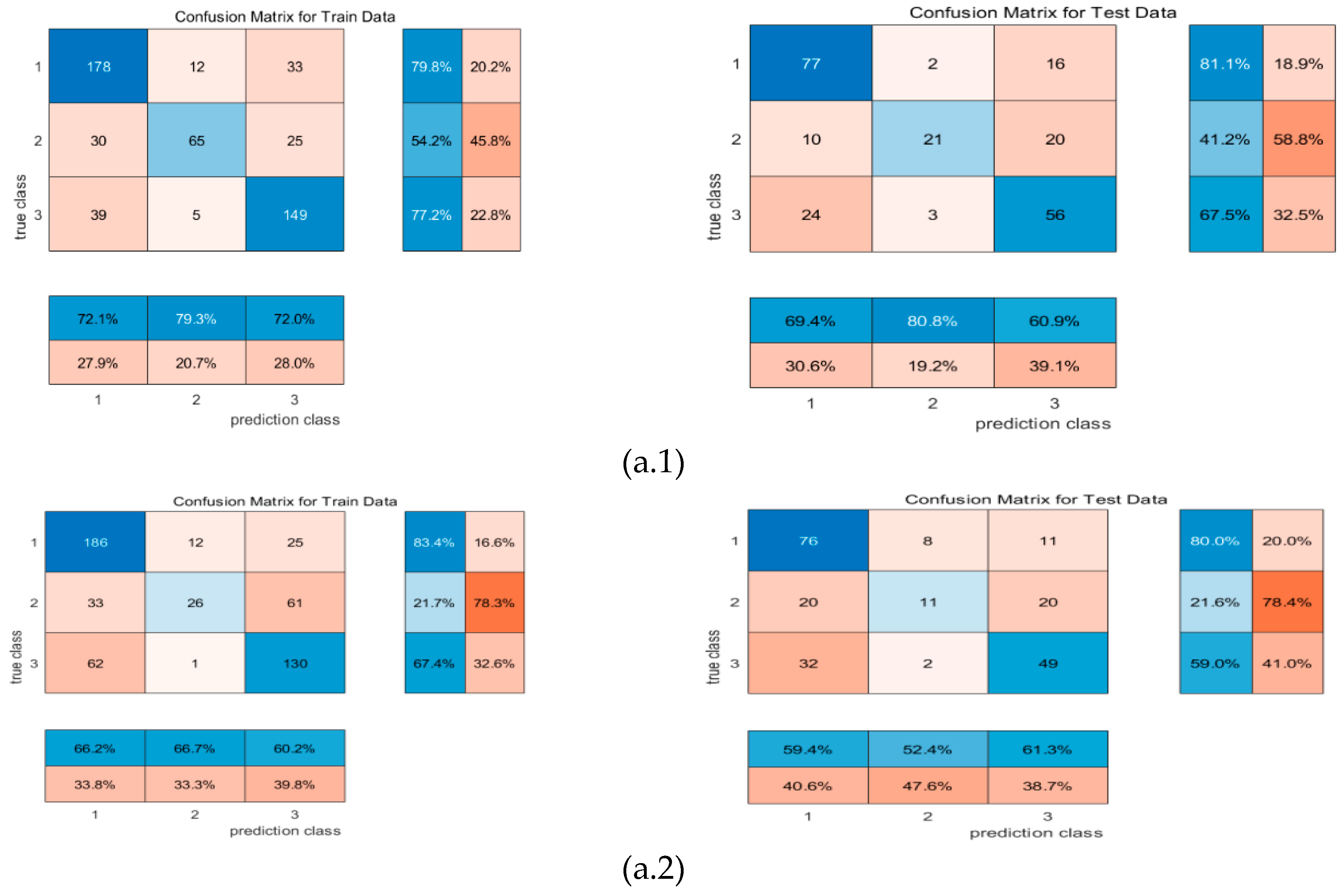
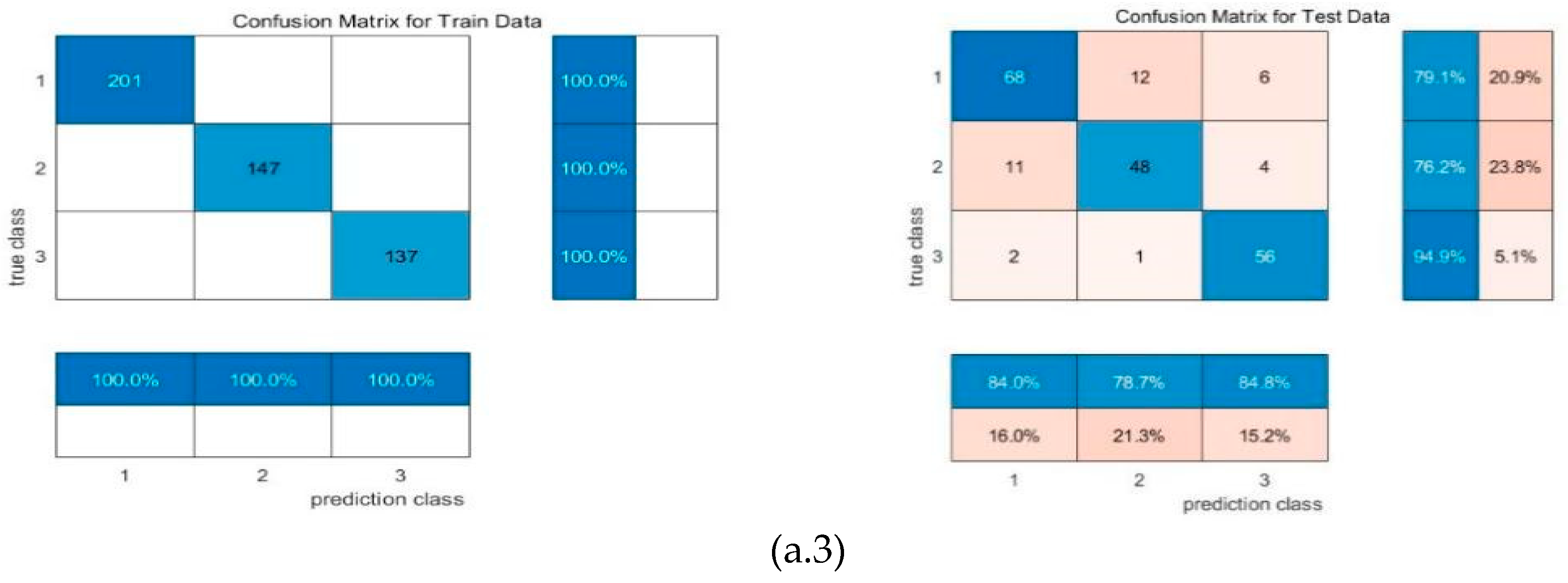
4.1. Confusion matrix
4.2. Accuracy
4.3. evaluation metrics for classification algorithms
4. Result
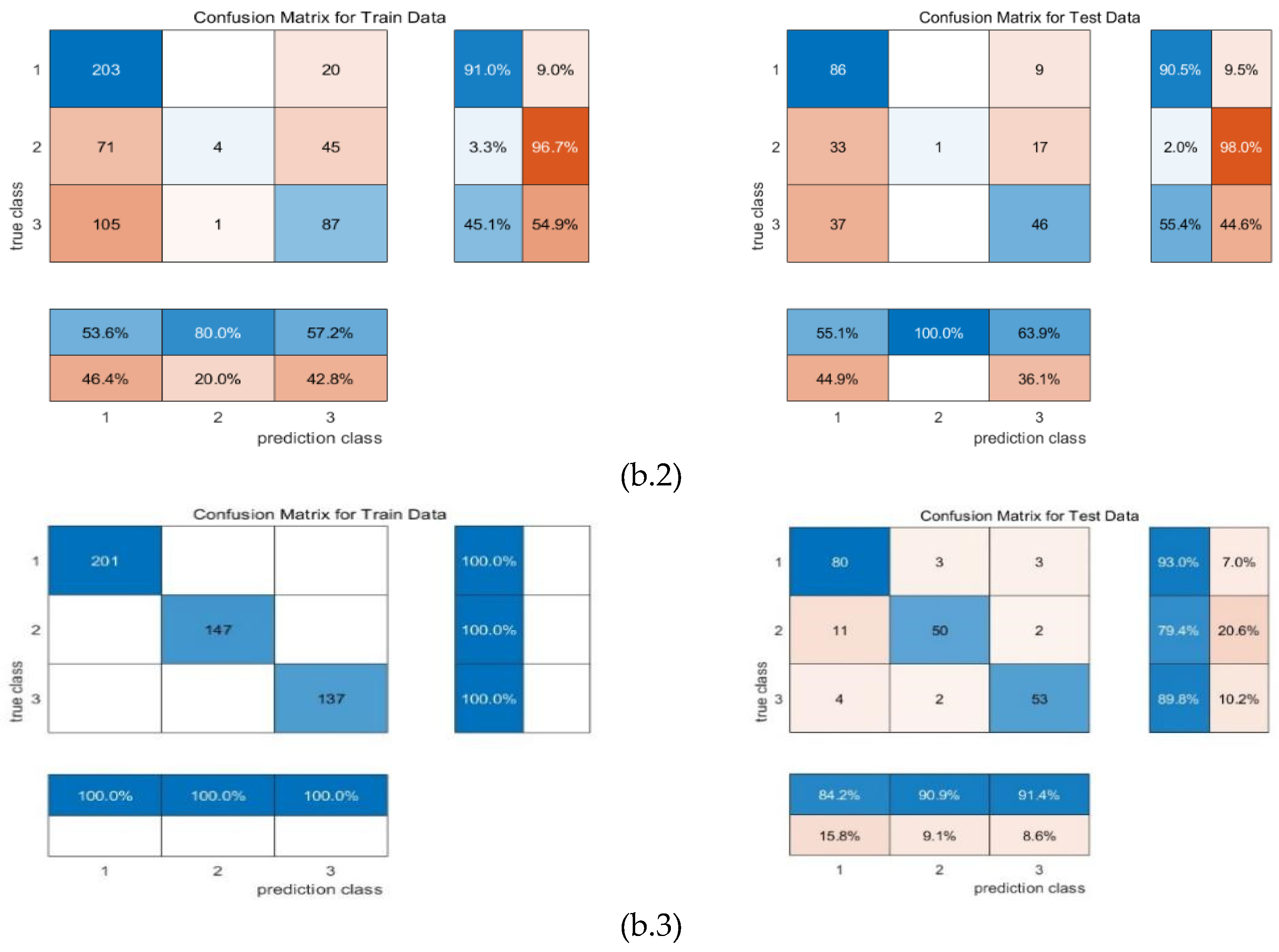
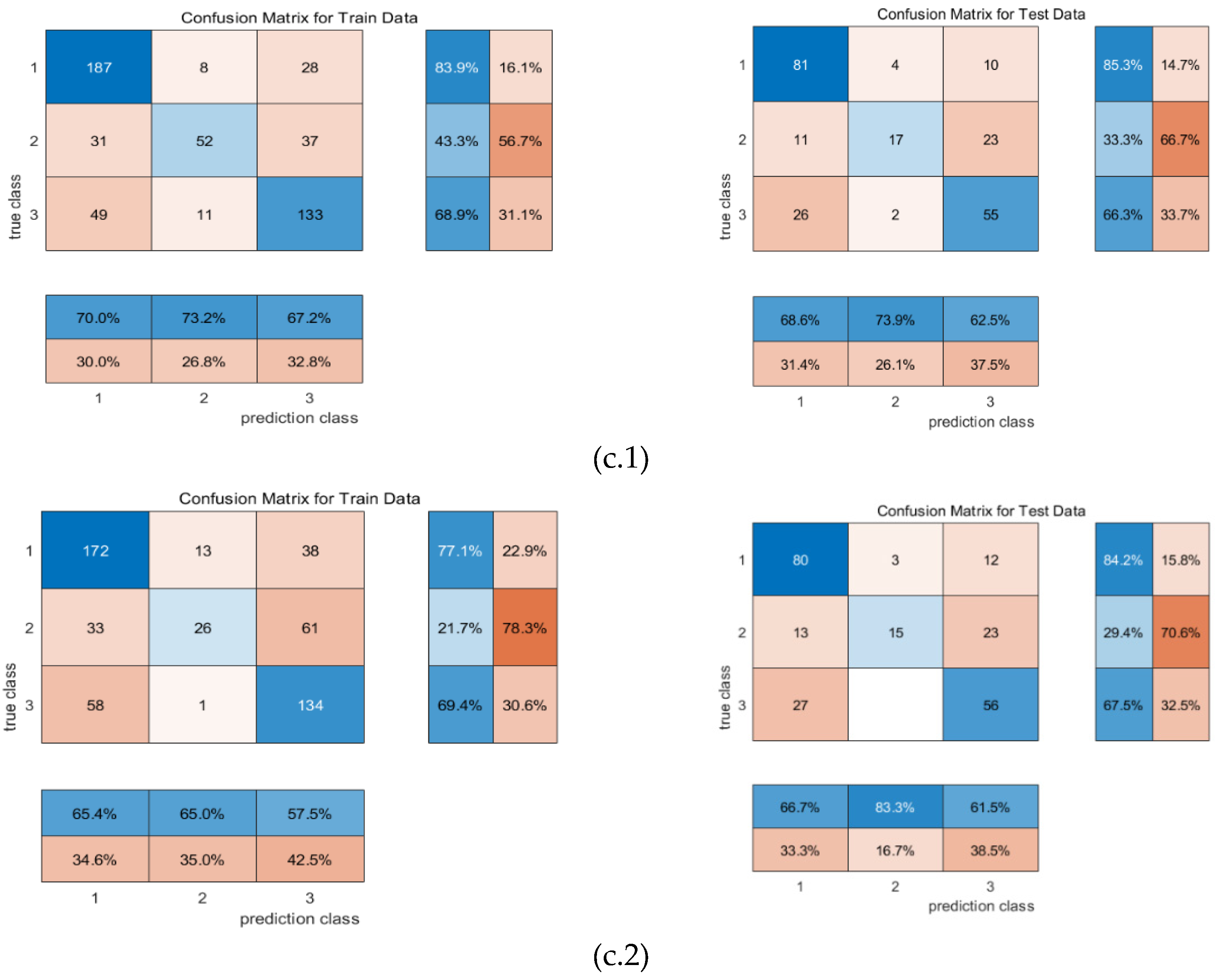
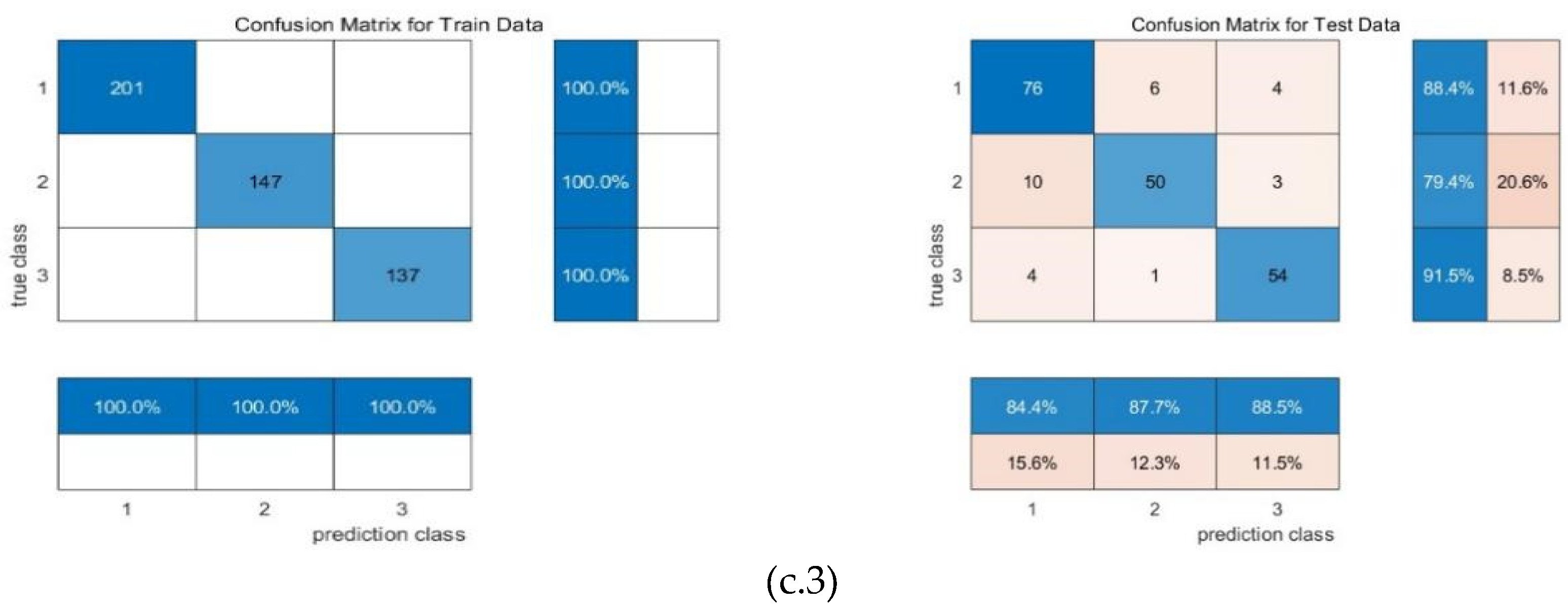
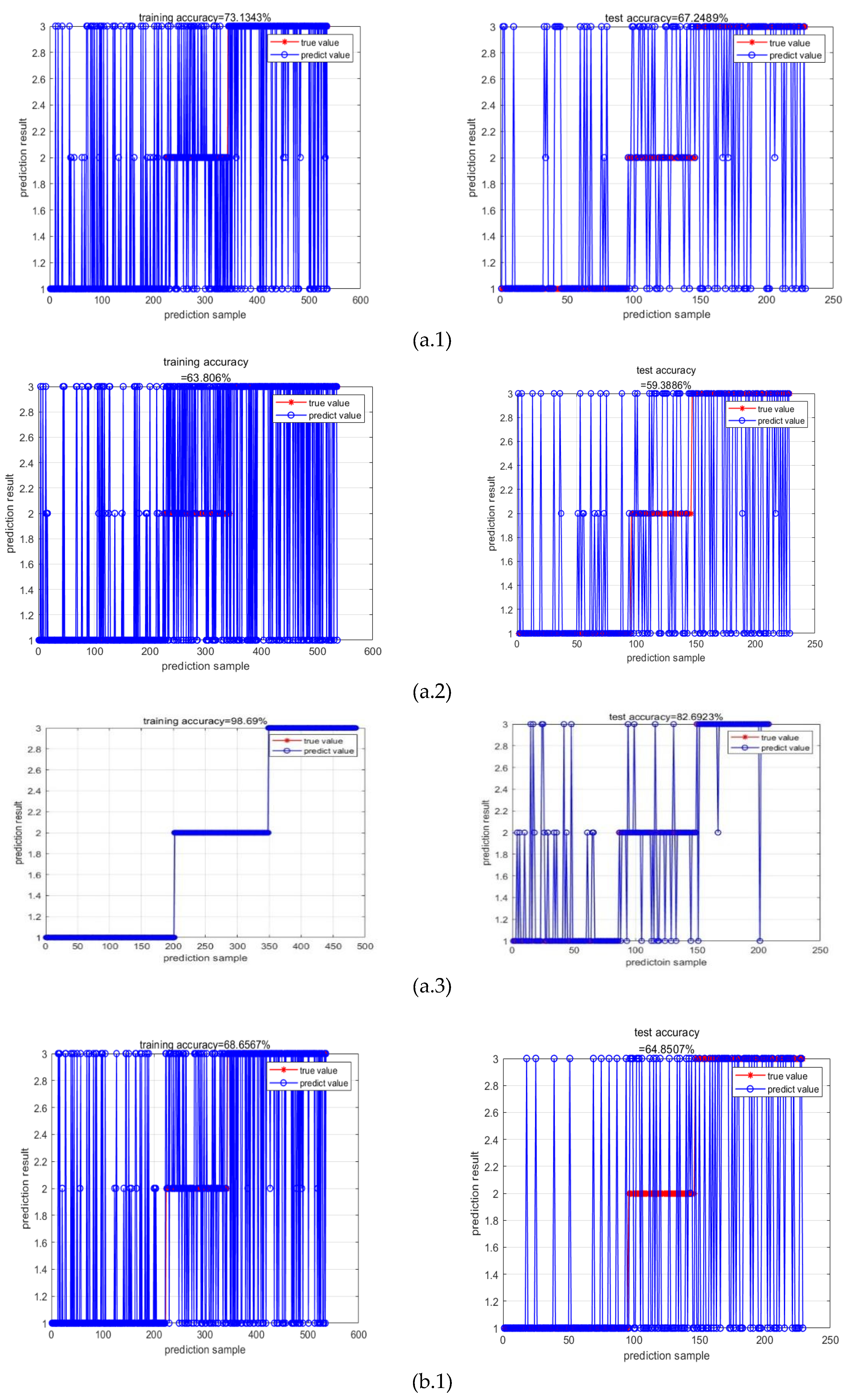
4. Conclusion and Discussion
Funding
Acknowledgments
Conflicts of Interest
Appendix A
References
- Ahmat, R.; Hasan, U.; Abliz, A.; Kasim, J. Hyperspectral estimate of Spring wheat leaf water content based on machine learning. Journal of Triticeae Crops 2021, 42, 640–648. [Google Scholar]
- Ahmed, M.; Yasmin, J.; Collins, W.; Cho, B. X-ray CT image analysis for the morphology of muskmelon seed in relation to germination. Biosyst. Eng 2018, 175, 183–193. [Google Scholar] [CrossRef]
- Albawi, S.; Mohammed, T.A.; Al-Zawi, S. Understanding of a convolutional neural network. In 2017 international conference on Engineering and Technology (ICET). IEEE. 2017; pp. 1-6. [CrossRef]
- Alkhamisi, M.A.; Khalaf, G.; Shukur, G. Some modifications for Choosing ridge parameter. Commun. Statist. Theor. Meth 2006, 35, 1–16. [Google Scholar] [CrossRef]
- Amatya, S.; Karkee, M.; Alva, A.; Larbi, P.; Adhikari, B. (2012). Hyperspectral Imaging for Detecting Water Stress in Potatoes. ASABE. Dallas, Texas, July 29 - August 1, 2012. St. Joseph, MI. [CrossRef]
- Ambrose, A.; Lohumi, S.; Lee, W.; Cho, B. Comparative nondestructive measurement of corn seed viability using Fourier transform near-infrared (FT-NIR) and Raman spectroscopy. Sens. Actuators, B Chem 2016, 224, 500–506. [Google Scholar] [CrossRef]
- Arau ́jo, M.; Saldanha, T.; Galva ̃o, R.; Yoneyama, T.; Chame, H.; Visani, V. Chemom. Intell. Lab. Syst 2001, 57.
- Baldwin, S.A.; Larson, M.J. An introduction to using Bayesian linear regression with clinical data. Behaviour research and therapy 2017, 98, 58–75. [Google Scholar] [CrossRef] [PubMed]
- Barbier, J.; Chen, W.K.; Panchenko, D.; Sáenz, M. Performance of Bayesian linear regression in a model with mismatch. arXiv arXiv:2107.06936, 2021.
- Barrs, H.; Weatherly, P.A. re-examination of the relative turgidity technique for estimating water deficits in leaves. Aus. J. Biol. Sci 1962, 15, 413–428. [Google Scholar] [CrossRef]
- Bishop, C.M.; Nasrabadi, N.M. Pattern recognition and machine learning (Vol. 4, No. 4, p. 738). New York: springer. 2006. [CrossRef]
- Bouvrie, J. (2006). Notes on convolutional neural networks.
- Canny, M.J.; Huang, C.X. Leaf water content and palisade cell size. New phytologist 2006, 170, 75–85. [Google Scholar] [CrossRef]
- Chang, C. (2007). Hyperspectral data exploitation: Theory and Applications. John Wiley; Sons. [CrossRef]
- Chen, Q.; Tang, B.; Long, Z.; Miao, J.; Huang, Z.; Dai, R.; Shi, S.; Zhao, M.; Zhong, N. Water quality classification using convolutional neural network based on UV-Vis Spectroscopy. Spectroscopy and Spectral Analysis 2022, 43. [Google Scholar]
- Cheng, G.; Han, J.; Lu, X. Remote sensing image scene classification: Benchmark and state of the art. Proc.IEEE 2017, 105, 1865–1883. [Google Scholar] [CrossRef]
- Cifre, J.; Bota, J.; Escalona, J.; Medrano, H.; Flexas, J. Physiological tools for irrigation scheduling in grapevine (vitis vinifera l. ): an open gate to improve water-use efficiency? Agriculture Ecosystems & Environment 2005, 106, 159–170. [Google Scholar] [CrossRef]
- Costa, J.; Grant, O.; Chaves, M. Thermography to explore plant-environment interactions. J. Exp. Bot. 2013, 64, 3937–3949. [Google Scholar] [CrossRef] [PubMed]
- Fei, S.; Chen, Z.; Li, L.; Ma, Y.; Xiao, Y. Bayesian model averaging to improve the yield prediction in wheat breeding trials. Agricultural and Forest Meteorology 2023, 328, 109237. [Google Scholar] [CrossRef]
- Ferentinos, K.P. Deep learning models for plant disease detection and diagnosis. Computers and Electronics in Agriculture 2018, 145, 311–318. [Google Scholar] [CrossRef]
- Ge, Y.; Bai, G.; Stoerger, V.; Schnable, J.C. Temporal dynamics of maize plant growth, water use, and leaf water content using automated high throughput RGB and hyperspectral imaging. Computers and Electronics in Agriculture 2016, 127, 625–632. [Google Scholar] [CrossRef]
- Gewali, U.; Monteiro, S.; Saber, E. (2018). Machine learning based hyperspectral image analysis: A survey. ArXiv abs/1802.08701.
- Giannoni, L.; Lang, F.; Tachtsidis, L. Hyperspectral imaging solutions for brain tissue metabolic and hemodynamic monitoring: past, current and future developments. Journal of Optics 2018, 20, 044009. [Google Scholar] [CrossRef] [PubMed]
- Golhani, K.; Balasundram, S.K.; Vadamalai, G.; Pradhan, B. Selection of a spectral index for detection of orange spotting disease in oil palm (Elaeis guineensis Jacq.) using red edge and neural network techniques. Journal of the Indian Society of Remote Sensing 2019, 47, 639–646. [Google Scholar] [CrossRef]
- Govender, M.; Govender, P.J.; Weiersbye, I.M.; Witkowski, E.T.F.; Ahmed, F. Review of commonly used remote sensing and ground-based technologies to measure plant water stress. Water Sa 2009, 35. [Google Scholar] [CrossRef]
- Govindjree, W.; Fork, D.; Armond, P. Chlorophyll a fluorescence transient as an indicator of water potential of leaves. Plant Sci. Letter 1981, 20. [Google Scholar]
- Gu, J.; Wang, Z.; Kuen, J.; Ma, L.; Shahroudy, A.; Shuai, B.; Liu, T.; Wang, X.; Wang, G.; Cai, J.; Chen, T. Recent advances in convolutional neural networks. Pattern recognition 2018, 77, 354–377. [Google Scholar] [CrossRef]
- Guifen, C.; Shan, Z.; Liying, C.; Siwei, F.; Jiaxin, Z. Corn plant disease recognition based on migration learning and convolutional neural network. Smart Agriculture 2019, 1, 34. [Google Scholar]
- Guretzki, S.; Papenbrock, J. Comparative analysis of methods analyzing effects of drought on the herbaceous plant Lablab purpureas. Journal of Applied Botany and Food Quality 2013, 86, 47–54. [Google Scholar]
- Halimu, C.; Kasem, A.; Newaz, S.H.S. (2019). Empirical Comparison of Area under ROC curve (AUC) and Mathew Correlation Coefficient (MCC) for Evaluating Machine Learning Algorithms on Imbalanced Datasets for Binary Classification Proceedings of the 3rd International Conference on Machine Learning and Soft Computing, Da Lat, Viet Nam. [CrossRef]
- Han, X.; Gui, X.; Yang, L. Introduction to the application and promotion of water and fertiliser integration technology in poor mountainous areas in poor mountainous regions of the north. Modern Horticulture 2018, 2, 232–233. [Google Scholar]
- He, B.; Han, Li.; Zhu, N.; Yu, J.; Qi, C.; Cai, L.; Gu, X. Effects of different irrigation strategies on growth and fruit trains of cherry and tomato. Vegetables 2022, 7. [Google Scholar]
- He, K.; Zhang, X.; Ren, S.; Sun, J. Identify mappings in deep residual networks. Computer Vision and Pattern Recognition. arXiv arXiv:1603.05027, 2016.
- Hernandez, J.; Lobos, G.; Matus, I.; del Pozo, A.; Silva, P.; Galleguillos, M. Using Ridge Regression Models to Estimate Grain Yield from Field Spectral Data in Bread Wheat (Triticum Aestivum L.) Grown under Three Water Regimes. Remote Sensing 2015, 7, 2109–2126. [Google Scholar] [CrossRef]
- How to use Pear. (2023). Chinese Medical Information Platform.
- Hoerl, A.E.; Kennard, R.W. Ridge regression: Biased estimation for non-orthogonal problems. Technometrics 1970, 12, 55–67. [Google Scholar] [CrossRef]
- Hu, W.; Huang, Y.; Wei, L. Deep Convolutional Neural Networks for Hyperspectral Image Classification[J]. Journal of Sensors 2015, 2, 1–12. [Google Scholar] [CrossRef]
- Jones, H.G. Irrigation scheduling: advantages and pitfalls of plant-based methods. J. Exp. Bot. 2004, 55, 2427–2436. [Google Scholar] [CrossRef]
- Junttila, S.; Hölttä, T.; Saarinen, N.; Kankare, V.; Yrttimaa, T.; Hyyppä, J.; Vastaranta, M. Close-range hyperspectral spectroscopy reveals leaf water content dynamics. Remote Sensing of Environment 2022, 277, 113071. [Google Scholar] [CrossRef]
- Kandpal, L.; Lohumi, S.; Kim, M.; Kang, J.; Cho, B. Near-infrared hyperspectral imaging system coupled with multivariate methods to predict viability and vigour in muskmelon seeds. Sensors and Actuators B: Chemical 2016, 229, 534–544. [Google Scholar] [CrossRef]
- Kang, Z.; Zhao, Y.; Chen, L.; Guo, Y.; Mu, Q.; Wang, S. Advances in Machine Learning and Hyperspectral Imaging in the Food Supply Chain. Food Eng Rev 2022, 14, 596–616. [Google Scholar] [CrossRef]
- Kang, Y.; Nam, J.; Kim, Y.; Lee, S.; Seong, D.; Jang, S.; Ryu, C. Assessment of regression models for predicting rice yield and protein content using unmanned aerial vehicle-based multispectral imagery. Remote Sensing 2021, 13, 1508. [Google Scholar] [CrossRef]
- Katsoulas, N.; Elvanidi, A.; Ferentinos, K.; Bartzanas, T.; Kittas, C. A hyperspectral imaging system for plant water stress detection: Calibration and Preliminary Results. Agricongress 2014.
- Khalaf, G.; Månsson, K.; Shukur, G. Modified ridge regression estimators. Communications in Statistics-Theory and Methods 2013, 42, 1476–1487. [Google Scholar] [CrossRef]
- Khalaf, G.; Shukur, G. Choosing ridge parameters for regression problems. Commun. Statist. Theor. Meth 2005, 34, 1177–1182. [Google Scholar] [CrossRef]
- Kibria, B. Performance of some new ridge regression estimators. Commun. Statist. Theor. Meth 2003, 32, 419–435. [Google Scholar] [CrossRef]
- Kong, D.; Zhu, J.; Duan, C.; Lu, L.; Chen, D. Bayesian linear regression for surface roughness prediction. Mechanical Systems and Signal Processing 2020, 142, 106770. [Google Scholar] [CrossRef]
- Lan, T.; Shen, S.; Yuan, H.; Jiang, Y.; Tong, H.; Ye, Y.A. Rapid Prediction Method of Moisture Content for Green Tea Fixation Based on WOA-Elman. Foods 2022, 11, 2928. [Google Scholar] [CrossRef]
- LeCun, Y.; Bottou, L.; Bengio, Y.; Haffner, P. Gradient-based learning applied to document recognition. Proceedings of the IEEE 1998, 86, 2278–2324. [Google Scholar] [CrossRef]
- Li, Z.; Liu, F.; Yang, W.; Peng, S.; Zhou, J. A survey of convolutional neural networks: analysis, applications, and prospects. IEEE transactions on neural networks and learning systems 2021. [CrossRef] [PubMed]
- Li, H.; Yang, W.; Lei, J.; She, J.; Zhou, X. Estimation of leaf water content from hyperspectral data of different plant species by using three new spectral absorption indices. PLoS ONE 2021, 16, e0249351. [Google Scholar] [CrossRef] [PubMed]
- Li, L.; Li, S.; Su, J.A. Multi-Category Brain Tumor Classification Method Bases on Improved ResNet50. CMC-Computers, Materials; Continua 2021, 69, 2355–2366. [Google Scholar] [CrossRef]
- Li, Y.; Wang, Z.; Liu, Y.; Li, Q.; Ding, Y.; Wang, Y.; Liu, M. Hyperspectral Estimation Model of Foliar Fe Concentration of Pyrus brestsschneideri Rehd. in Different Periods. Southwest China Journal of Agricultural Sciences 2019, 32, 1. [Google Scholar]
- Li, Y. Models of estimating nutrient elements in leaves and canopy of Pyrus sinkiangensis ‘Kuerlexiangli’ using hyperspectral data.Xin Jiang Agricultural University. 2018. [CrossRef]
- Li, M.; Chu, R.; Yu, Q.; Abu, I.; Shuren, C.; Shen, S. Evaluating structural, chlorophyll-based and photochemical indices to detect summer maize responses to continuous water stress. Water 2018, 10, 500. [Google Scholar] [CrossRef]
- Liou, C.Y.; Lin, S.L. Finite memory loading in hairy neurons. Natural Computing 2006, 5, 15–42. [Google Scholar] [CrossRef]
- Liou, C.Y. (2006). Backbone structure of hairy memory. In Artificial Neural Networks–ICANN 2006: In 16th International Conference, Athens, Greece, September 10-14, 2006. Proceedings, Part I 16 (pp. 688-697). Springer Berlin Heidelberg. [CrossRef]
- Liu, Y.; Lyu, Q.; He, S.; Yi, S.; Liu, X.; Xie, R.; Zheng, Y.; Deng, L. Prediction of nitrogen and phosphorus contents in citrus leaves based on hyperspectral imaging. International Journal of Agricultural and Biological Engineering 2015, 8, 80–88. [Google Scholar]
- Liu, Y.; Zhang, G.; Liu, D. Simultaneous Chlorophyll and Water Content Measurement in Navel Orange Leaves Based on Hyperspectral Imaging. Spectroscopy 2014, 29. [Google Scholar]
- Liu, L.; Tao, H.; Fang, J.; Zheng, W.; Wang, L.; Jin, X. Identifying anthracnose and black spot pear leaves on near-infrared hyper spectroscopy. Journal of Agricultural Machinery 2022, 53, 2. [Google Scholar]
- Luo, Y.; Zou, J.; Yao, C.; Zhao, X.; Li, T.; Bai, G. (2018). HSI-CNN: A novel convolution neural network for hyperspectral image. In 2018 International Conference on Audio, Language and Image Processing (ICALIP) (pp. 464-469). IEEE. [CrossRef]
- Luo, H.; Liu, Y. (2017, November). A prediction method based on improved ridge regression. In 2017 8th IEEE International Conference on Software Engineering and Service Science (ICSESS) (pp. 596-599). IEEE. [CrossRef]
- Ma, T.; Tsuchikawa, S.; Inagaki, T. Rapid and non-destructive seed viability prediction using near-infrared hyperspectral imaging coupled with a deep learning approach. Computers and Electronics in Agriculture 2020, 177, 105683. [Google Scholar] [CrossRef]
- Matdoan, M.Y.; Wance, M.; Balami, A.M. (2021, September). Ridge regression modeling in overcoming multicollinearity problems in multiple linear regression models (case study: Life expectancy in Maluku Province). In AIP Conference Proceedings (Vol. 2360, No. 1). AIP Publishing.
- Mirjalili, S.; Mirjalili, S.; Lewis, A. Grey wolf optimizer[J]. Advances in engineering software 2014, 69, 46–61. [Google Scholar] [CrossRef]
- Nair, V.; Hinton, G.E. (2010). Rectified linear units improve restricted boltzmann machines. In Proceedings of the 27th international conference on machine learning (ICML-10) (pp. 807-814).
- Netto, A.; Campostrini, E.; De Oliveira, J.; Bressansmith, R. Photosynthetic pigments, nitrogen, chlorophyll a fluorescence and SPAD-502 readings in coffee leaves. Sci. Hortic 2005, 104, 199–209. [Google Scholar] [CrossRef]
- O’Shea, K.; Nash, R. An introduction to convolutional neural networks. arXiv arXiv:1511.08458, 2015.
- Pandey, P.; Ge, Y.; Stoerger, V.; Schnable, J.C. High throughput in vivo analysis of plant leaf chemical properties using hyperspectral imaging. Frontiers in plant science 2017, 8, 1348 https://doi org/103389/fpls201701348. [Google Scholar] [CrossRef]
- Pacheco-Gil, R.A.; Velasco-Cruz, C.; Pérez-Rodríguez, P.; Burgueño, J.; Pérez-Elizalde, S.; Rodrigues, F.; Ortiz-Monasterio, I.; del Valle-Paniagua, D.H.; Toledo, F. Bayesian modelling of phosphorus content in wheat grain using hyperspectral reflectance data. Plant Methods 2023, 19, 1–11. [Google Scholar] [CrossRef] [PubMed]
- Pear. (2023). Encyclopedia of China Publishing House.
- Pinkard, E.; Patel, V.; Mohammed, C. Chlorophyll and nitrogen determination for plantation-grown Eucalyptus nitens and Eucalyptus globules using a non-destructive meter. For. Ecol. Manage 2006, 223, 211–217. [Google Scholar] [CrossRef]
- Pontes, M.; Galva ̃o, R.; Arau ́jo, M.; Moreira, P.; Neto, O.; Jos(e) ́, G.; Saldanha, T. Chemom. Intell. Lab. Syst. 2005, 78. [Google Scholar]
- Poobalasubramanian, M.; Park, E.-S.; Faqeerzada, M.A.; Kim, T.; Kim, M.S.; Baek, I.; Cho, B.-K. Identification of Early Heat and Water Stress in Strawberry Plants Using Chlorophyll-Fluorescence Indices Extracted via Hyperspectral Images. Sensors 2022, 22, 8706 MDPI AG Retrieved from. [Google Scholar] [CrossRef]
- Rayapudi, S.R.; Lakshmi, N.; Manyala, R.R.; Srinivasa, R.A. Optimal Network Reconfiguration of Large-Scale Distribution System Using Harmony Search Algorithm. IEEE Transactions on Power Systems 2011, 26, 1080–1088. [Google Scholar] [CrossRef]
- Renzullo, L.A. method of wavelength selection and spectral discrimination of hyperspectral reflectance spectrometry. IEEE Trans. Geosci. Remote Sens 2006, 44, 1986–1994. [Google Scholar] [CrossRef]
- Rumelhart, D.E.; McClelland, J.L.; PDP Research Group, C.O.R.P.O.R.A.T.E. (Eds.). (1986). Parallel distributed processing: Explorations in the microstructure of cognition, Vol. 1: Foundations. MIT press.
- Sabour, S.; Frosst, N.; Hinton, G.E. (2017). Dynamic routing between capsules. In Advances in neural information processing systems (pp. 3856-3866). 3856–3866.
- Sak, H.; Senior, A.; Beaufays, F. Long Short-Term Memory Based Recurrent Neural Network Architectures for Large Vocabulary Speech Recognition. Neural and Evolutionary Computing. arXiv arXiv:1402.1128, 2014.
- Santos, L.; Barreto, W.O.; Silva, E.F. (2016). Araújo. Wilson, S.
- Shu, Z.; Li, X.; Liu, Y. Detection of Chili Foreign Objects Using Hyperspectral Imaging Combined with Chemometric and Target Detection Algorithms. Foods 2023, 12, 2618. [Google Scholar] [CrossRef] [PubMed]
- Silva, G.; Medeiros, T.; Lia, B.; Antonio, C. Origin, Domestication, and dispersing of pear (Pyrus spp.). Advances in Agriculture 2014, 1–8. [Google Scholar] [CrossRef]
- Sriram, L.M.K.; Gilanifar, M.; Zhou, Y.; Ozguven, E.E.; Arghandeh, R. Causal Markov Elman network for load forecasting in multinetwork systems. IEEE Transactions on Industrial Electronics 2018, 66, 1434–1442. [Google Scholar] [CrossRef]
- Suhandono, N.; Mulyono, S.; Maspiyanti, F.; Fanany, M.I. (2013). An extreme leaning machine model for growth stages classification of rice plants from hyperspectral images subdistrict indramayu. In The Second Indonesia-Japanese Conference on Knowledge Creation; Intelligent Computing. [CrossRef]
- Thilagaraj, M.; Arunkumar, N.; Ramkumar, S.; Hariharasitaraman, S. Electrooculogram signal identification for elderly disabled using Elman network. Microprocessors and Microsystems 2021, 82, 103811. [Google Scholar] [CrossRef]
- Tipping, M.E. (2003). Bayesian inference: An introduction to principles and practice in machine learning. In Summer School on Machine Learning (pp. 41-62). Berlin, Heidelberg: Springer Berlin Heidelberg. [CrossRef]
- Verrelst, J.; Alonso, L.; Caicedo, J.; Moreno, J.; Camps-Valls, G. Gaussian Process Retrieval of Chlorophyll Content From Imaging Spectroscopy Data. IEEE Journal of Selected Topics in Applied Earth Observations and Remote Sensing 2013, 6, 867–874. [Google Scholar] [CrossRef]
- Visa, S.; Ramsay, B.; Ralescu, A.; Knaap, E. (2011). Confusion Matrix-based Feature Selection (Vol. 710).
- Wang, Y.; Li, L.; Shen, S.; Liu, Y.; Ning, J.; Zhang, Z. Rapid detection of the quality index of postharvest fresh tea leaves using hyperspectral imaging. Journal of the Science of Food and Agriculture 2020, 100, 3803–3811. [Google Scholar] [CrossRef] [PubMed]
- Wang, T. (2022). Inversion of nitrogen and chlorophyll content in crop leaves based on hyperspectral and machine learning. Jilin University. [CrossRef]
- Wang, Y.; Wang, L.; Yang, F.; Di, W.; Chang, Q. Advantages of direct input-to-output connections in neural networks: The Elman network for stock index forecasting. Information Sciences 2021, 547, 1066–1079. [Google Scholar] [CrossRef]
- Wang, Y.; Li, L.; Shen, S.; Liu, Y.; Ning, J.; Zhang, Z. Rapid detection of the quality index of postharvest fresh tea leaves using hyperspectral imaging. Journal of the Science of Food and Agriculture 2020, 100, 3803–3811. [Google Scholar] [CrossRef]
- Wang, Z.; Hu, M.; Zhai, G. Application of deep learning architectures for accurate and rapid detection of internal mechanical damage of blueberry using hyperspectral transmittance data. Sensors 2018, 18, 1126. [Google Scholar] [CrossRef] [PubMed]
- Wang, X.; Shi, G.; Xu, Q. Toxic effects of lanthanum, cerium, chromium and zinc on potamogeton malaianus[J]. Journal of The Chinese Rare Earth Society 2004, 22, 682–686. [Google Scholar]
- Wei, Y.; Li, X.; He, Y. Generalisation of tea moisture content models based on VNIR spectra subjected to fractional differential treatment. Biosystems Engineering 2021, 205, 174–186. [Google Scholar] [CrossRef]
- Wen, L.J.; Asaari, M.S.M.; Dhondt, S. Spectral Correction and Dimensionality Reduction of Hyperspectral Images for Plant Water Stress Assessment. Science; Technology 2023. [CrossRef]
- Weng, S.; Ma, J.; Tao, W.; Tan, Y.; Pan, M.; Zhang, Z.; Huang, L.; Zheng, L.; Zhao, J. Drought stress identification of tomato plant using multi-features of hyperspectral imaging and subsample fusion. Frontiers in plant science 2023, 14, 1073530. [Google Scholar] [CrossRef] [PubMed]
- Woldegiorgis, S.; Enqvist, A.; Baciak, J. ResNet and CycleGAN for pulse shape discrimination of He-4 detector pulse: Recovering pulses conventional algorithms fail to label unanimously[J]. Applied Radiation and Isotopes 2021, 6, 109819. [Google Scholar] [CrossRef] [PubMed]
- Wu, X.; Zhao, X.; Chen, R.; Liu, P.; Liang, W.; Wang, J.; Teng, M.; Wang, X.; Gao, S. Wastewater treatment plants act as essential sources of microplastic formation in aquatic environments: A critical review. Water Research 2022, 221, 118825. [Google Scholar] [CrossRef] [PubMed]
- Yalcin, H.; Razavi, S. (2016, July). Plant classification using convolutional neural networks. In 2016 Fifth International Conference on Agro-Geoinformatics (Agro-Geoinformatics) (pp. 1-5). IEEE. [CrossRef]
- Yamashita, R.; Nishio, M.; Do, R.K.G.; Togashi, K. Convolutional neural networks: an overview and application in radiology. Insights into imaging 2018, 9, 611–629. [Google Scholar] [CrossRef] [PubMed]
- Yang, W. (2020). Ningxia Lingwu Horticultural Experimental Field (Lingwu Forest Farm). Atlas of Fruit Tree Germplasm Resources of Ningxia Lingwu Horticultural Experimental Field[M].
- Yang, J.; Li, J. (2017). Application of deep convolution neural network. In 2017 14th International Computer Conference on Wavelet Active Media Technology and Information Processing (ICCWAMTIP) (pp. 229-232). IEEE. [CrossRef]
- Zhao, D.; Li, Z.; Feng, G.; Wang, F.; Hao, C.; He, Y.; Dong, S. Using swarm intelligence optimization algorithms to predict the height of fractured water-conducting zone. Energy Exploration; Exploitation 2023, 01445987231178938. [CrossRef]
- Zhao, T.; Nakano, A. Agricultural Product Authenticity and Geographical Origin Traceability. Jpn. Agric. Res. Q. JARQ 2018, 52, 115–122. [Google Scholar] [CrossRef]
- Zhao, T.; Nakano, A.; Iwaski, Y.; Umeda, H. Application of hyperspectral imaging for assessment of tomato leaf water status in plant factories. Applied Sciences 2020, 10, 4665, doi 103390/app10134665. [Google Scholar] [CrossRef]
- Zhu, H.; Chu, B.; Zhang, C.; Liu, F.; Jiang, L.; He, Y. Hyperspectral imaging for presymptomatic detection of tobacco disease with successive projections algorithm and machine-learning classifiers. Scientific reports 2017, 7, 4125. [Google Scholar] [CrossRef]
- Zhu, Q.; Guan, J.; Huang, M.; Lu, R.; Mendoza, F. Predicting bruise susceptibility of ‘Golden Delicious’ apples using hyperspectral scattering technique. Postharvest Biology and Technology 2016, 114, 86–94. [Google Scholar] [CrossRef]
| Date | July 25 (day 0) |
July 27 (day 1) |
July 29 (day 3) |
July 31 (day 5) | August 1 (day 7) |
| Number of images collected | 30 for normal treatment | 90 (30 normal, 30 overwater, 30 drought) per day |
|||
| Band8 | Band15 | Band54 | Band64 | Band67 | Band78 | Band96 |
| 395.55nm | 409.75nm | 489.53nm | 510.19nm | 516.40nm | 539.23nm | 576.81nm |
| Input data | HSI whole data cube 300×(30+90×4) |
| Main spectra 7×(30+90×4) | |
| CNN features of main spectra 4096×(30+90×4) |
| Neural network | parameters |
| RR-MLR | gam = 10 |
| Bayesian Linear Regression | sigma_squared=0.01 |
| Elman Neural Network | epochs = 2000 goal = 1e-5 lr = 0.01 |
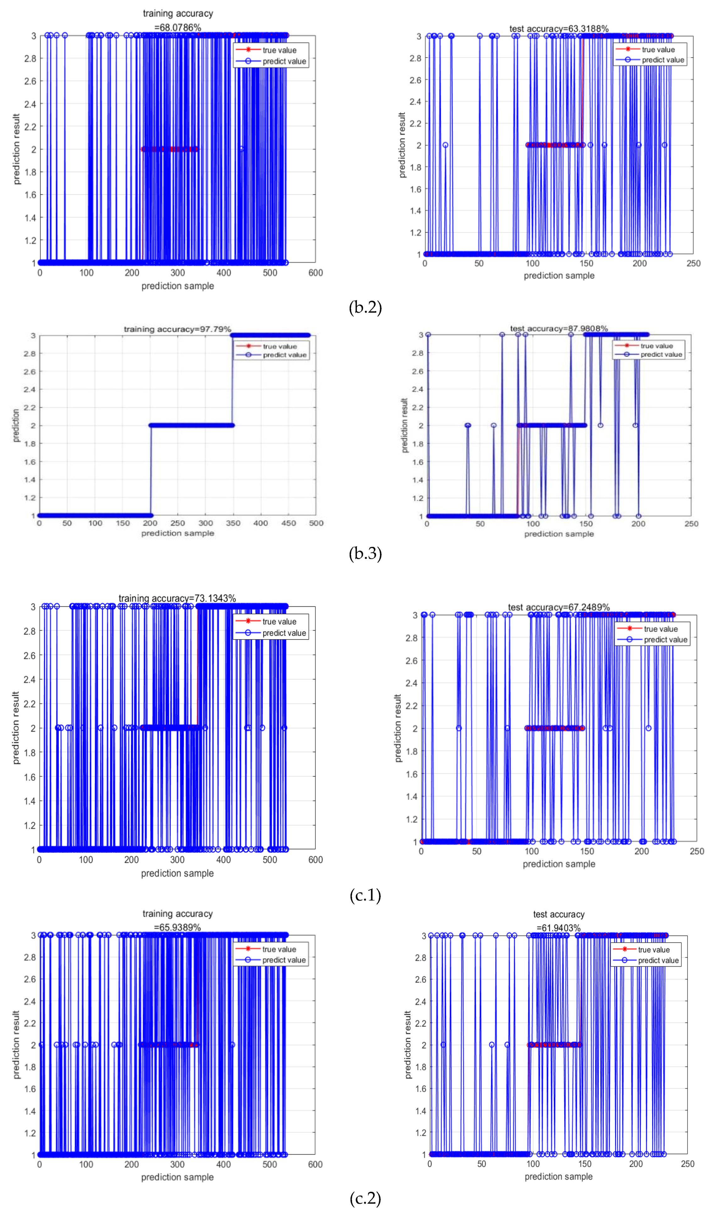
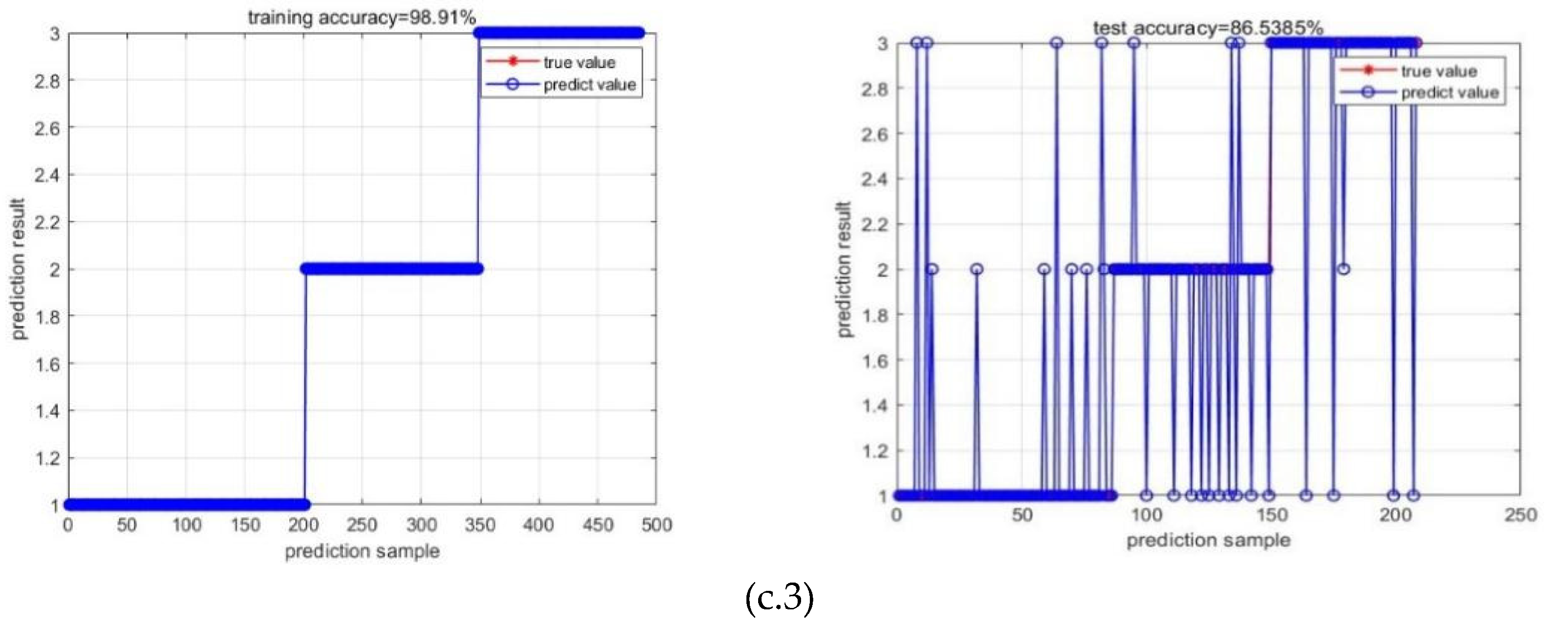
| Machine learning | input | F1 | precision | recall | mse_loss | test accuracy |
| RR-MLR | Whole datacube | 0.65 | 0.66 | 0.64 | 0.80 | 67.25% |
| Key wavelengths | 0.60 | 0.67 | 0.60 | 0.80 | 59.39% | |
| CNN feature | 0.86 | 0.86 | 0.86 | 0.19 | 82.69% | |
| Bayes | Whole datacube | 0.72 | 0.68 | 0.77 | 0.91 | 64.85% |
| Key wavelengths | 0.59 | 0.51 | 0.69 | 1.39 | 63.32% | |
| CNN feature | 0.87 | 0.84 | 0.91 | 0.23 | 87.98% | |
| Elman | Whole datacube | 0.65 | 0.66 | 0.65 | 0.16 | 67.25% |
| Key wavelengths | 0.57 | 0.66 | 0.57 | 0.17 | 61.94% | |
| CNN feature | 0.87 | 0.87 | 0.87 | 0.08 | 86.54% |
Disclaimer/Publisher’s Note: The statements, opinions and data contained in all publications are solely those of the individual author(s) and contributor(s) and not of MDPI and/or the editor(s). MDPI and/or the editor(s) disclaim responsibility for any injury to people or property resulting from any ideas, methods, instructions or products referred to in the content. |
© 2024 by the authors. Licensee MDPI, Basel, Switzerland. This article is an open access article distributed under the terms and conditions of the Creative Commons Attribution (CC BY) license (http://creativecommons.org/licenses/by/4.0/).


