
You are currently viewing a beta version of our website. If you spot anything unusual, kindly let us know.
Preprint
Article
Smart City Scenario Editor for General What-if Analysis
Altmetrics
Downloads
86
Views
70
Comments
0
A peer-reviewed article of this preprint also exists.


Abstract
Nowadays cities, due to the increasing urbanization, are facing challenges spanning on multiple domains as mobility, energy, environment, etc. Big data gathered from legacy systems, from geographic information systems, operators, and Internet of Things technologies can be exploited to provide insights to assess the current status of a city, the possibility to perform what-if analysis to observe the impact of possible changes. The few available solutions for formal scenario definition and analysis are limited to single domain analysis and provide proprietary formats and tools. Therefore, in this paper, we present a novel scenario model and editor integrated into the open-source Snap4City.org platform to define general processing and what-if scenarios in order to carry out analysis on different domains. The proposed solution responds to a series of identified requirements and implements NGSIv2 compliant data models and formal description of the urban context. As a case of study, a traffic congestion analysis is provided, confirming the validity and usefulness of the proposed solution.
Keywords:
Subject: Engineering - Transportation Science and Technology
1. Introduction
Thanks to the increasing deployment of Internet of Things (IoT) technologies and the availability of big data, the concept of smart city is nowadays widely applied worldwide to address current and future challenges in the urban context. Indeed, due to the increasing urbanization, city councils are called to plan and take actions in several domains like mobility [1,2], urban infrastructures [3], energy [4], security [5,6], environment [7], etc. Smart city IoT platforms [8,9] with interactive dashboards [10] and advanced urban digital twin interfaces [11,12] are fundamental tools to assess the current and past states of the cities. However, such technologies should be improved by including solutions for tactic and strategic plans which have to consider predictions and simulations capabilities to help the decision makers in the urban development. In particular, the introduction of what-if analysis solutions [13] to observe the impacts of possible changes to the current urban scenario are required to offer decision makers effective decision support system (DSS) tools. Such solution should provide a structured framework for data-driven decision-making processes leveraging on advanced algorithms and real-time data integration to allow the users to experiment and evaluate the impacts of changes in the urban environment. The first step is to introduce such variations into the representation used to describe smart city entities (roads, buildings, services, green areas, etc.), for example modelled with ontologies or relational databases [14,15]. Therefore, a graphical interface to alter the current representation and formalize a set of hypothetical scenarios, i.e., a scenario editor, according to which assess impacts and effects of city policies in terms of Key Performance Indicators (KPI) and metrics is mandatory.
In the literature, it is possible to find proposals addressing the formalization of scenarios and corresponding editor tools mainly in the context of autonomous driving [16,17], where simulations are carried out to evaluate system response to specific conditions, e.g., complex maneuvers involving multiple vehicles. The formalization of scenario is also useful to decompose the problem for fog and edge computing [18,19]; for shaping context for computation and action [20]; contextualizing and shaping the user behavior [21], etc. A solution could be usage of classic GIS (Geographic Information Systems) tools, e.g., QGIS [22] and ArcGIS [23], in which the definition of shape is possible, and IoT, POI (point of interests), services, and other references may be loaded. However, GIS software tools are typically very far to provide tools for editing the road graph with corresponding semantic information such as priority, lanes, restrictions, velocity, etc., and are far to produce scenario descriptors which can be used for simulation/computation; many other data have to be added. In that context, standards to formalize a scenario emerged, such as the ASAM OpenSCENARIO [24] used in conjunction with the ASAM OpenDRIVE [25] and OpenCRG [26] standards, to describe static and dynamic characteristics. On the other hand, more general tools and models which should be able to cope with a wider concept of city scenarios seem to be less investigated. Some solutions with specific capabilities have been proposed as commercial or open-source software. For example, the OpenStreetMap (OSM) ecosystem provides the iD editor [27], a web-based editor to modify OSM map elements in an intuitive manner. However, the introduced changes are directly incorporated into the OSM database, limiting the possibility of producing multiple scenarios to be analyzed simultaneously at the basis of computation and machine learning (ML) or artificial intelligence (AI) solutions/simulation. In addition, the area of interest of the OSM scenario is not formally defined to be directly exploited for successive computations and/or simulations and need to be extracted by means of complex SQL queries. More advanced models and tools are proposed by SUMO [28], and PTV for Vissim [29] and Visum [30] simulators. SUMO is an open-source traffic simulator and includes as scenario editor the so-called SUMO netedit tool [31]. It allows to add, modify, and remove roads and connections as well as change the element attributes, such as number of lanes, speed limits, etc. Different file formats are accepted as input and output, including the OpenDRIVE standard. PTV Vissim and Visum are two proprietary simulators, for micro and macro scales, respectively. Both solutions include a similar editor where the user can define changes to the current scenario by altering the road network. However, both SUMO and PTV editor requires on-premises installation, while a web-based interface would be preferable for easiest access and wider distribution. Moreover, none of the available solution can automatically extract and integrate information coming from IoT sensors time series, an important source typically available in smart city environments, that can be used to extend the focus of the simulation from the traffic to other problems like pollution, waste management, index computation, etc.
In this paper, the development of a model for scenarios and corresponding web based open-source tool for scenario editing are presented. To this end, a collection of requirements has been identified and reported. From the scenario editor, the user can select an area of interest and modify the topology and the attributes of the road network. Then, different kind of IoT devices, entities, and services can be recalled and selected n order to complete the formalization of the scenario for computing and analysis phases. The aim was the definition of a powerful scenario model and tool which can be used to define the context for a huge number of context-depended computational activities (in time and space) such as those for computing people flows, traffic flow reconstructions, heatmaps, origin destination matrices, indicators, navigation, representation, etc., maybe extracting information from multiple big data spaces, knowledge bases/graphs, etc., and allowing the users to produce also hypothetical scenarios/contexts on which the computation/simulation could be performed, as in the what-if analysis. The formalization of scenarios in a flexible manner enables the assessment of the impact of changes in complex city contexts. The modeling of the scenario itself could change its status (e.g., proposed, approved, closed), evolving over time, and be shared among experts and decision makers. In the proposed scenario management, the model definition and structure is formalized as a smart data model compatible with the NGSIv2 standard for data exchange and indexed into a knowledge base for future retrieval via semantic queries [14]. In this paper, the requirements and the formalization of the scenario and editor are presented. In addition, a case study is provided in which the scenario model and tool are used to define the context and needed to compute the traffic flow reconstruction of a portion of the city, in actual conditions and by changing some constraints enabling in this case the fast re-computation/simulation for what-if analysis. The proposed scenario model and editor have been developed and are integrated into the Snap4City platform (https://www.snap4city.org/), an open-source IoT platform able to manage multiple tenants and billions of data with the key focus on interoperability (the tool is accessible from dashboards such as [32]). The scenario editor is embedded as a novel module of Dashboard Builder Multi Data Map widget [33] and is able to retrieve static (road graph, urban elements, sensor positions, etc.) and real-time (sensor readings, public transport time schedules, weather, temperature, etc.) data though specific APIs.
The main contributions of this paper are:
- The definition of a series of requirements that a scenario editor must meet;
- The definition of the smart data model describing a scenario and a formal model to describe the road network;
- The development of an open-source web-based scenario editor, and its integration into the Snap4City platform;
- A case study to show the scenario editor functionalities applied to the traffic flow reconstruction problem, to validate the scenario model and tool.
This paper is organized as follows. In Section 2, the general architecture and data flow related to the scenario model and editor is presented. In Section 3, the requirements defined to guide the development of the scenario model and editor are provided, together with the formal definition of a scenario as a smart data model. In Section 4, the Scenario Editor is described. Section 5 presents a case of study where the scenario model and editor is used to perform traffic flow reconstruction and congestion analysis for what-if analysis. Finally, in Section 6 conclusions are drawn. This research has been performed in the context of MOST National Center on Sustainable Mobility in Italy [34], Snap4City is one of the reference platforms for the CN MOST.
2. Context definition
Figure 1 depicts a conceptual block diagram describing the workflow for scenario production and evaluation, therefore defining the operative context for the scenario editor. As can be seen, the user interacts with the scenario editor interface by specifying the area of interest, datetime, metadata, loading and selecting real or simulated data (sensors, services), etc., and may be altering the current scenario in all details. All the data are retrieved from Snap4City storage by performing queries on Km4City knowledge base or any other storage. The produced scenario, with or without modifications, with respect to a current condition, may be saved, exported/imported, shared according to a smart data model (see Section 3.1) and can be readily used as input to compute KPIs and metrics, as, for example, the evaluation of heatmaps on the basis of sensors data into the scenario, or computing a 15-minute city index [35]. The same or multiple scenarios can be used in input to one or more data analytic processes to compute traffic flow reconstructions, pollutant predictions, people flows, simulations such as the traffic flow reconstruction [36], the computation of heatmaps [37], the management of waste [38], etc. Analytic results are then passed to the KPI and metric computations to quantify the impact of the produced scenarios, to compare the value of those KPI/metrics in the current situation with respect to the modified scenario according to the changes as in What-if analysis. Finally, obtained results and comparison are shown to the user.
Note that, the scenario editor can take as input a previously created scenario (see yellow arrows in Figure 1) that the user can further modify to obtain a novel version of the same scenario, create a new scenario derived from the old one, or change the operative status of the scenario, e.g., from proposed to approved or rejected status. This approach opens the path for collaborative work on what-if analysis, city development and study [39,40].
Moreover, some analytics can require additional information (pink arrows in Figure 1). In this case the scenario is presented again to the user that specifies the missing information and change the processing status of the scenario, e.g., from init to under analysis. Using the scenario versioning and status is possible to save and track the history/evolution of a scenario model and reduce the work of the users. To give the reader an example, let us now to suppose that due to scheduled street works some roads should be closed to traffic and the city council must find the best solution to avoid congestions. The mobility operator of the city has to assess the impact and find a solution, he/she starts by creating a first scenario, , by closing some roads to traffic to study what happen if those changes are performed. Then, is loaded into the editor and the user adds further changes, such as inverting some road travel directions, creating a scenario . The operator loads again and this time changes the number of lanes of some roads to create the scenario .and are derived scenarios from and both have version set to v0 and operating status to proposed. and are sent to the traffic flow reconstruction to assess which is the better solution to limit traffic congestion due to the closed roads. The city chief of the mobility operators decides is not a valid solution: the operative status of passes to rejected. At the same time, the city council requires further changes to that the user implements, updating the version of to v1. After a second round of reconstruction and computation of KPIs, is accepted and its operative status moves to approved. Thus, the formal definition of robust model for scenarios is the first step to create also automated models and tool to AI based tools for automated generation of best scenarios which in any case have to be verified and selected from the mobility city chief.
3. Requirement Analysis and Scenario Data Model Definition
In this Section, the identified functional and non-function requirements for the development of the Scenario Editor are presented and discussed. Functional requirements are reported in Table 1, with ID, name, and a brief description, while non-functional requirements are discussed in the following.
As can be seen in Table 1, eleven functional requirements have been defined. Since scenario editing is performed on geographical areas, a ground map and associated controls are required (R01). Requirements from R02 to R04 are needed to define the specific context for the scenario. These include the drawing of the area of interest, the description of metadata, the selection of the knowledge base or storages from where to fetch the data. Requirements R05 and R06 describes the main viewing and editing functionality available to the user, from the selection of the data to consider, to their manipulation in order to define alterations of the current scenario. Note that, according to R07, a scenario editor must allow to load (and modify) heterogeneous data so as to be exploitable with multiple analytics and KPIs to perform different kinds of what-if analyses. Since the editor allows the operators alter entities and roads as well as select different areas, a check of consistency (R08) should be carried out to avoid the creation of unrealistic scenario: for example, unreachable road segments due to wrong travel direction assignments. There should be the possibility of creating scenarios with different statuses and versions (R09): a processing status progression could be required by specific analytics, requiring user intervention on different steps of the process. On the other hand, the scenario operative status and version could be used to describe the evolution of the scenario and track the introduced changes, may be revert. Therefore, the scenario editor should provide the possibility to create and save the scenario, and to load a previously defined scenario (for example to define a new version or to advance the scenario status) and save it with a new name (R10). Finally, the scenario editor must produce a scenario conformant to a given model that should be sufficiently elastic to accommodate additional variables (R11).
Some non-functional requirements must also be defined. At first, the editor should be implemented as a web application, to avoid the need for installing software and guarantee a wide accessibility and coworking. High level of performance should be achieved both in terms of quick response times to offer a seamless interactivity, high reliability, and availability to avoid service interruption. Security and privacy aspects must also be considered: this requires the implementation of adequate management of user profiles with different roles and with different organizations to which any user can be associated with. Moreover, the possibility to delegate or make public the access to data, defined scenarios, or analysis results is required to enable multiple users to work on the same problem in a collaborative way. For example, an operator could prepare different scenarios and results and then delegate/share them to the office manager/chief who takes the final decision.
To satisfy all the non-functional requirements and some of the functional ones (R01, R04, R05, R06, R07) the proposed scenario editor has been integrated into the open-source IoT platform Snap4City. The platform includes functionalities to collect data from different sources though push and pull modalities using brokers, gateways, and services, and to index them in the Km4City knowledge base [14], and shadow store the data in an OpenSearch cluster. Using specific APIs, data can be retrieved using spatial, temporal, and relational queries, therefore addressing R04, R05, and R06. Multiple analytical methods (R07) are available as well as solutions to compute KPIs based on Node-RED flows according to national and international specifications like the SUMP [41], Italian PUMS [42] and European SUMI [43]. Moreover, Snap4City is GDPR [44] compliant and successfully passed several penetration tests, uses multiple user’s roles, handles different organizations, implements data and service ownership functionalities with the possibility to change ownership, delegate, or make the resources available for given organizations or to the public. The main installation uses up-to-date redundancy solutions to guarantee a high level of reliability. The proposed scenario editor is integrated as an extension of the multi data map of the DashboardBuilder to create a map widget with navigation controls (R01) and can be included in any Snap4City dashboard and accessed with any web browser.
3.1. Scenario data model
Hereafter a formal definition of the data model for a smart city scenario is provided, responding to requirement R11. Such definition was developed to store the needed data and information according to the functional requirements presented in the previous section. A scenario is described as a context entity compliant with the FIWARE NGSIv2 specification [45], with a type SmartCityScenario and an ID defined as an URI, corresponding to an entity instance in the knowledge base. A scenario has the following attributes (with data types reported in brackets):
- A1.
- name (string): the name of the scenario;
- A2.
- description (string): a brief description of the scenario;
- A3.
- location (string): the textual name of the geographic area considered;
- A4.
- startDatetime (string): timestamp of the starting instant from which the scenario is valid, represented as ISO string;
- A5.
- endDatetimes (string): timestamp of the last time instant for which the scenario is valid, represented as ISO string;
- A6.
- areaOfInterest (geometry): a polygon describing the portion of the city over which the scenario is defined, represented as GeoJSON;
- A7.
- knowledgeBase (string): the ID of the knowledge base used to fetch the data in the scenario, represented as URI. It also identifies an Organization or tenant in the multitenant Snap4City platform
- A8.
- entities (data structure): IoT devices or other urban entities (e.g., traffic sensors, semaphores, POIs, buildings, gardens, waste bins, etc.) considered in the scenario and included in the area of interest, represented as JSON. Each entity is identified with an URI associated to an instance in the knowledge base;
- A9.
- roads (geometry): a list of roads included in the area of interest, represented as a GeoJSON, according to the formal model described in Section 3.2. Each road is identified with an URI associated with an instance in the knowledge base;
- A10.
- restrictions (data structure): a list of traffic or access restrictions applied to entities and roads of the scenario, represented as JSON;
- A11.
- additionalData (data structure): data required by specific analytics, represented as JSON;
- A12.
- processingStatus (data structure): a list indicating the status of the scenario for each used analytic, represented as a JSON. Each list entry can assume different values depending on the analytic to which it is referred;
- A13.
- operativeStatus (string): a description indicating the status of the scenario; it can assume the following values: proposed, approved, rejected;
- A14.
- version (string): the version of the scenario, used to implement a versioning system. Please note that an automated versioning approach based on time is implemented by using dateObserved attribute;
- A15.
- dataObserved (string): timestamps of the creation/ modifications of the scenario, represented as ISO string.
Attributes A1 – A5 describe the metadata of the scenario, responding to requirement R03. A6 is used to store the area of interest (R02), while in A7 the URI of the reference knowledge base is set (R04). To satisfy R05 and R06, attributes A8, A9, and A10 are used to store respectively the entities, the roads, and the restrictions included in the scenario and possibly modified. R07 and R11 are addressed with attribute A11, used to store possible additional data required by analytics or KPIs. A12 is used to track the processing steps reached with some analytics. Finally, A13, A14, and A15 are related to requirements R09 and R10 to take into account different operative statuses and versions.
In order to respond to requirement R08, in the next section, a formal method to assess the validity of the (possibly modified) road graph included in a scenario is presented.
3.2 Formal road graph data model
In this section, the formal representation of the road graph of the scenario model is presented in order to: facilitate reasoning and formal verifications over the road graph, as well as to provide a formal framework to define KPIs involving the road graph and data connected via knowledge base.
Full Road Graph definition. The full road graph (FRG) is defined as a tuple
where:
- is the set of nodes forming the road graph (i.e. the road junctions);
- is the set of edges of the road graph, where means that there is a physical link allowing to go from node v to node w and vice versa,
- R is the set of roads,
- is a function associating a GPS position to each node,
- is a function associating to each edge the road it belongs to,
- is a function stating for each edge the direction it can be traversed, means it can be traversed in both ways, only from to , only from to ;
- is a function associating for each edge the number of lanes (>0),
- is a function to associate each edge with its max speed.
- models turn restrictions where tuple means that the restriction of type applies to the edge via the node to edge , the node has to be shared between edges and , for example restriction means that from edge it is not possible to turn to edge .
The FRG is used to represent all the detailed road shapes, and from this it can be built the Compact Road Graph (CRG) where edges connected in a sequence having the same associated data (dir, road, lanes, max_speed) can be represented as a single edge. For this purpose, we introduced the following functions:
where eq. (2) returns the set of edges that are insisting on edge , while eq. (3) gives the set of edges that are next to . Symbol is a projection function used to get the i-th component of a tuple/sequence, i.e., and provides the last element of a sequence. Function on a sequence provides the subsequence without the last element.
Compact Road Graph definition. Given a FRG as in eq. (1) its compact version (CRG), is expressed as
And it can be built by introducing an additional mapping function that maps each edge of the compact version to a sequence of edges of the full version. With the following constraints:
- , the set of nodes of the compact version are a subset of the full version,
-
and
- maps to the longest possible sequence of edges
Whether, in the compact graph, there exist edges having only one next edge, i.e., , means that there exists an edge on the road where the direction or the number of lanes or the max speed or the road name are changing.
Note that, with respect to a naïve graph modelling of the road network, the FRG or the CRG representations are required in order to take into account the possible restrictions. Then, in order to assess, if a road graph (full or compact) is meaningful, some standard graph algorithms can be used to check for example the number of connected components or to find the shortest path between two nodes since in a well-designed road network all nodes should be reachable from all the other nodes.
4. Scenario Editor
The Scenario Editor was developed and enforced in Snap4City tools according to the requirements presented in Section 3, with the aim of providing a versatile and easy-to-use operator tool for defining, studying, and analyzing smart city scenarios [32]. In Figure 2, a screenshot of a Snap4City dashboard including the proposed scenario editor is provided. As can be seen, a map is used as background while on the left and right sides of the map are placed panels and buttons that can be used to create the scenario. The save functionality is accessible on to registered users, and the registration is free of charge.
The editor can work in edit and view modalities (see the button in the bottom-left corner of the map): the former is the modality to define a scenario and introduce changes, the latter is used to display previously created scenarios, received in delegation of made public. On the right side, a panel to specify scenario metadata is displayed, including fields for the scenario name, location, description, reference knowledge base, analytics and KPI to use, start and end datetimes of the scenario validity. In the top-left corner, under the buttons to set the map zoom level, controls to draw a squared or polygonal shape are provided. After having defined the shape of the area of interest, the road graph is retrieved from the specified knowledge base and shown over the map with interactive graphical elements. Roads are displayed with arrows specifying the travel direction and with different color to indicate if roads are not in use (gray, not to be considered in the scenario processing), if they are with a single (blue) or double (red) travel direction. Each road segment can be clicked to access and modify specific information (category, number of lanes, max speed, etc.). Using the button in the bottom-left corner, roads can be modified by creating, splitting, or deleting segments, dragging and joining nodes. Undo and redo actions are implemented to help the user in correcting possible errors. Entities are requested using the selector menu on the left side of the dashboard. Each selector entry specifies an entity kind (traffic, weather, air quality sensors, POIs, bus stops, etc.) that can be loaded independently into the scenario editor. Once the user completes the editing operations, the resulting scenario can be saved using the format described in Section 3.1.
Before saving the scenario, the system performs a consistency check on the defined road graph to highlight possible errors using the formal method described in Section 3.2. In the case the consistency check fails -- e.g., when nodes with only entering roads are detected, an alert is sent to the user and the different components are highlighted in the map. Additionally, a warning is given to the user when the system detects roads having segments with different number of lanes or different max speeds. Even if, this is something that may happen in real cases, due to the relevance of such characteristics, the system highlights suspicious cases to help the user avoiding introducing errors in the scenario.
In the next section, as case study, about the usage of the scenario editor for traffic flow reconstruction and what-if analysis is presented.
5. Case of Study: Traffic Flow Reconstruction
Understanding the evolution of traffic within urban environments is important for effective city planning and management to face the challenges posed by growing populations and increasing vehicular density, or to address events and planned activities on the urban infrastructure. Accurate insights into how traffic patterns evolve over time enable decision-makers to implement strategic measures that enhance mobility, reduce congestion, and improve overall urban resilience. In this context, the traffic flow reconstruction case study presents a comprehensive approach, utilizing the scenario editor and data-driven tools to analyze and reconstruct traffic flow in the area of interest, performing what-if analysis, and therefore contributing to informed decision-making.
The proposed scenario editor is used to select a specific area of the map, retrieve information about the road network and traffic sensors, and possibly to apply changes, defining a new scenario for traffic analysis. The scenario editor allows the users to choose which sensors take into account for the traffic reconstruction procedure, or to assign some reference time trends. Traffic flow reconstruction (TFR) is carried out exploiting the algorithm presented in [36] that is based on the solution of a fluid dynamic problem based on partial differential equations (PDEs). As usual in PDE problem solutions, boundary conditions must be specified: in this case the reconstruction method requires to know the traffic flow entering the area of interest. For this reason, the scenario editor automatically detects road sections that intersect the area of interest and whose direction is entering in the area. On these points virtual traffic sensors are placed, in which the user can specify 24 hours trends to be used as input. Different kinds of traffic time trends can also be exploited, as for example typical time trends generated from historical traffic data, predicted typical time trend data, or arbitrary time trends defined by the user. Once completed the editing process, the scenario is saved according to the defined data model (see Section 3.1), with the scenario processing status attribute set to init. Then, the user can load the scenario in the TFR analytic, and a first pre-processing phase can be carried out: road intersections connected to only two road segments with same number of lanes and max speed are removed and the related road segment merged, passing from a FRG to a CRG (see Section 3.2). This reduces the fragmentation of the road network, helping in the required discretization of the numerical solution (see [36] for further details). After this phase the scenario is updated: attribute A9 now describe the CRG, and the processing status moves to merged. Then, additional inputs are requested from the user. The scenario is loaded into the editor, and the user is asked to set the road segment capabilities (i.e., an estimate of the number of vehicles that a road can accommodate). Such information is exploited to compute the so-called Traffic Distribution Matrices (TDM) that represent how vehicles are distributed at road junctions. More precisely, so that and , for and , where coefficients (called weights) are the percentages of vehicles arriving from the -th incoming road and taking the -th outcoming road (assuming that, on each junction, the incoming flux coincides with the outcoming flux). The scenario is saved again, with road capabilities and TDM saved in the additionalData attribute (A11), and the processing status set to ready. Now the TFR can run on the updated scenario to compute the traffic reconstruction.
To assess the correctness and the validity of the proposed approach, two tests were carried out. At first, we study the correspondence between a TFR computed on a wide road network, i.e., the whole city of Florence (Italy), and the reconstruction obtained on a small sub-graph, i.e., the scenario area of interest, to evaluate traffic flow discrepancy (see Section 5.1). Then, in a second test we assessed the impact of alterations in the road graph by changing road travel directions to create additional paths with the objective of reducing congestion on the principal roads (see Section 5.2).
5.1. Consistency and correctness of TFR
A first assessment analysis has been performed to assess the correctness of the TFR. A small area of the city of Florence (see Figure 3a) has been selected to test if the TFR results are consistent with the one extrapolated by the traffic flow reconstruction computed on [36] in the small/micro-scale scenario. The historical traffic flow reconstruction computed in the 28th September 2023, referred as , has been chosen for the analysis.
Using the scenario editor, the area of interest has been selected (see Figure 3b). On the area of interest, the scenario provides the road elements on which the historical reconstruction was performed. The virtual sensors were considered to reproduce the same boundary conditions and they have been initialized with flow values of for the considered road segments, inside the area. The traffic sensors inside the scenario have also been considered and the same TDMs has been imposed to obtain the small-scale reconstruction for the defined scenario, referred as . The reconstruction at 9:00 am on 2023-09-28 is reported in Figure 3c.
The TFR algorithm produced almost identical traffic flow reconstruction results on the defined micro-scale scenario with respect to the macro scale, showing an equal level of congestion on the corresponding road elements. In Figure 4 is reported the charts with the historical traffic flow reconstruction values and the TFR at 9:00 on 2023-09-28 where 68 road segments of 20m are compared. The reconstructions show a high degree of correspondence. In average, a mean absolute error of 0.05648 (cars/20m) was achieved, demonstrating the robustness of the TFR method and the validity of the proposed approach passing from macro to micro scale computation. The mean historical value for reference was 0.734774 (cars/20m) and the error performed is about 6.81%. Note that, we could not achieve perfectly identical results since in the selected sub-graph generated a different merged graph with respect to , and, as consequence, the reconstructions worked on slightly different road segments in length, preventing a perfect match between and road graphs.
5.2. What-If analysis for traffic congestion reduction
In this second test, we exploited the scenario editor to perform what-if analysis on traffic flows. The chosen area is the same on which has been performed the consistency and correctness analysis and is reported in Figure 3b, referred as version whose graph structure is reported in Figure 5. This area is often congested in the main roundabout and in Figure 5 this road sections are highlighted in red. Measurements for real traffic sensors encompassed in the area, and for the virtual sensors on the border were sampled from historical data. No changes were introduced in the road network.
With the aim of improving the traffic flow in the selected area using the editor, it has been possible to study an alternative road network configuration, version , by inverting the travel directions for streets: Borgo Pinti, via Giuseppe Giusti, and via Vittorio Alfieri. The new path should alleviate the traffic flow moving from north to south, redirecting a part of the traffic on alternative path. The graph structure of is also reported in Figure 5. The value related to TDM estimation of Matteotti was set to 70, and the Pinti one to 12. This means that in percentage 14.63% or cars should take Pinti as route and the remaining 85.36% should continue on the roundabout, according to the weight coefficient in the TDM. To complete the possible scenario versions another one has been considered taking and changing the value of Pinti from 12 to 25 in the TDM. Meaning that: what if more cars would choose that route? In detail, what would happen if instead of around 15% the percentage of vehicles choosing Pinti was in this case 26.32% increasing of about 10%.
According to What-If analysis, we tested if the new configuration could improve the traffic jam in the selected area, it has been performed the TFR for , , whose reconstructions are reported in Figure 6. As can be seen, by having created a new route, the congestion on the main road decrease with respect to . However, from the graphs in Figure 6 it is possible to note that in there is still a 20m segment in heavy traffic flow state (represented in red), meanwhile in no congestion is visible on the main road.
To quantify the improvements, we divided the road segments in four groups, depending on the measured traffic density in the initial scenario w.r.t. the critical density (equal to half the maximum density, i.e. ): FreeFlow, if ; FluidFlow, if ; HeavyFlow, if ; VeryHeavyFlow, if . Note that, traffic flow and density are related with the following equation:
where is the maximum velocity.
In Figure 7, the traffic density for the 24 hours in the four groups for , , are reported. The trends reveal the decrease of the number of road segments in the Very Heavy traffic status from to and . However, the differences between and are less evident from the trend graph. The results have also been reported numerically in Table 2 that contains the average values (h24) for the different states in the different versions of the scenario considered. The major improvement can be seen in the percentage of segments in the Fluid Flow state with respect to and , rising from to 0.1501 to 0.1705 and 0.1744 respectively. Even if the percentage of segments in the Heavy Flow state slightly increases in the modified versions this is acceptable since it determines an important decrease in the segments in the Very Heavy Flow from 0.0455 in to 0.0274 of and 0.0223 in .
To evaluate the overall improvement in the traffic in the defined scenarios specific delta metrics for the different traffic density states have been defined as follows:
- ,
- ,
- ,
Please note that, if and are positive, then the number of segments (in percentage) having uncongested traffic states decrease passing from the original scenario to the modified one. Generally, the occurrence of a positive value in (and assumes a negative effect. Thus, when and are negative values, the traffic state is improved between the compared scenarios. This means that, the uncongested traffic state increases passing from the original scenario to the modified one. Vice-versa, if and are positive, then the uncongested traffic state decreases during the scenarios’ comparison.
In order to evaluate the percentage of improvement according to FreeFlow, FluidFlow, HeavyFlow, VeryHeavyFlow traffic states, we have to consider a multiplicative contribution factor according to the above dissertation. Then, -1 in cases of FRrs and FLrs estimations, while 1 when HErs and VHer are considered. For example, in order to estimate the percentage of improvement of the scenario with respect to the original one, we consider the following formula for FRrs, where -1:
Similarly, different states are evaluated, and the related estimation is reported in Table 3. The results demonstrate that, with respect to scenarios , and reduced the proportion of segment in the VeriHeavyFlow state of 39.86% and 50.98% respectively, and at the same time, augment percentage of segments in the FluidFlow class by 13.69% and 16.27% respectively. On the other hand, the segments in the FreeFlow status reduce, and those in HeavyFlow augment. However, such negative impact is very slightly compared to the benefits obtained, that significantly reduce the overall congestion, in particular on the main roads.
Finally, in Table 4 the execution times for the three scenarios are reported. Computations have been carried out on a workstation equipped with an Intel i7 CPU, with 32 GB of RAM. No GPU was used. As can be seen the TFR computation for 24h results is around 160 seconds with a slight difference between the three versions.
6. Conclusions
In this paper a novel scenario model and editor have been presented. The solution has been designed according to a large range of smart city requirements analysis for covering relevant cases in computing scenario based: metrics, KPI, heatmaps, traffic flow, etc. The editor, responding to a series of requirements and implementing standard data models and formal method analysis, allows the user to load and visualize the road network and other entities in a specific area and give the possibility to alter the current status to define multiple what-if scenarios. A case study has been presented, involving the production of a scenario for traffic congestion analysis showing how the proposed solution could be effectively used to realize a decision support system to help city councils and decision makers to answer the current and future necessities of a smart city. The formalization of the scenario allowed to pass from macro to micro scale computation without losing of generality for the traffic flow. Thus, analytic software, already implemented and accessible in the Snap4City open-source platform, can be used to carry out predictions, simulations, and reconstructions to assess the impact of changes in different domains (e.g., mobility, energy, environment) in terms of different possible KPIs and metrics. The scenario editor is accessible and can be tested on Snap4City.org. It is presently in use on the research and development activities of the CN MOST in Italy. CN MOST is the national Center on Sustainable Mobility in Italy.
Author Contributions
Conceptualization, P.N.; methodology, P.B., S.B., M.F. and P.N; software, L.A., D.B. and E.C.; validation, S.B., D.B., E.C., M.F. and P.N; formal analysis, P.B., S.B., M.F. and P.N; investigation, S.B., E.C., M.F. and P.N.; data curation, P.B. and M.F.; writing—original draft preparation, P.B., S.B., E.C., M.F. and P.N.; writing—review and editing, M.F. and P.N.; visualization, E.C. and M.F.; supervision, S.B., M.F. and P.N.; project administration, P.B., M.F. and P.N.; funding acquisition, P.N. All authors have read and agreed to the published version of the manuscript.
Funding
This research was financed by the European Union—NextGenerationEU (National Sustainable Mobility Center CN00000023, Italian Ministry of University and Research Decree n. 1033— 17/06/2022, Spoke 9).
Institutional Review Board Statement
Not applicable.
Informed Consent Statement
Not applicable.
Data Availability Statement
Not applicable.
Acknowledgments
The authors would like to express a sincere thanks to the MIUR, CN MOST. A special thanks to the many developers working on the Snap4City platforms. Snap4City (https://www.snap4city.org, accessed 31 January 2024) and Km4City are open technologies of the DISIT Lab.
Conflicts of Interest
No conflicts of interest are involved among the authors.
References
- Torre-Bastida, A. I., Del Ser, J., Laña, I., Ilardia, M., Bilbao, M. N., & Campos-Cordobés, S. (2018). Big Data for transportation and mobility: recent advances, trends and challenges. IET Intelligent Transport Systems, 12(8), 742-755. [CrossRef]
- Bellini, P., Bilotta, S., Collini, E., Fanfani, M., & Nesi, P. (2024). Data Sources and Models for Integrated Mobility and Transport Solutions. Sensors, 24(2), 441. 2. [CrossRef]
- Hodson, M., Marvin, S., Robinson, B., & Swilling, M. (2012). Reshaping urban infrastructure: Material flow analysis and transitions analysis in an urban context. Journal of Industrial Ecology, 16(6), 789-800. [CrossRef]
- Keirstead, J., Jennings, M., & Sivakumar, A. (2012). A review of urban energy system models: Approaches, challenges and opportunities. Renewable and Sustainable Energy Reviews, 16(6), 3847-3866. [CrossRef]
- Gharaibeh, A., Salahuddin, M. A., Hussini, S. J., Khreishah, A., Khalil, I., Guizani, M., & Al-Fuqaha, A. (2017). Smart cities: A survey on data management, security, and enabling technologies. IEEE Communications Surveys & Tutorials, 19(4), 2456-2501. [CrossRef]
- Collini, E., Palesi, L. A. I., Nesi, P., Pantaleo, G., & Zhao, W. (2023). Flexible thermal camera solution for Smart city people detection and counting. Multimedia Tools and Applications, 1-29. [CrossRef]
- Charnes, A., Cooper, W. W., & Li, S. (1989). Using data envelopment analysis to evaluate efficiency in the economic performance of Chinese cities. Socio-Economic Planning Sciences, 23(6), 325-344. [CrossRef]
- C. Garau, P. Nesi, I. Paoli, M. Paolucci, P. Zamperlin, A Big Data Platform for Smart and Sustainable Cities: Environmental Monitoring case studies in Europe. Proc. Of International Conference on Computational Science and its Applications, ICCSA2020. Cagliari, Italy, 1-4 July 2020. 4 July.
- Krylovskiy, A., Jahn, M., & Patti, E. (2015, August). Designing a smart city internet of things platform with microservice architecture. In 2015 3rd international conference on future internet of things and cloud (pp. 25-30). IEEE.
- Q. Han, P. Nesi, G. Pantaleo, I. Paoli, “Smart City Dashboards: Design, Development and Evaluation”, Proc. Of the IEEE ICHMS 2020, International Conference on Human Machine Systems, September 2020. 20 September 2020.
- Adreani, L., Bellini, P., Colombo, C., Fanfani, M., Nesi, P., Pantaleo, G., & Pisanu, R. (2023). Implementing integrated digital twin modelling and representation into the Snap4City platform for smart city solutions. Multimedia Tools and Applications, 1-26. [CrossRef]
- Jafari, M., Kavousi-Fard, A., Chen, T., & Karimi, M. (2023). A review on digital twin technology in smart grid, transportation system and smart city: Challenges and future. IEEE Access. [CrossRef]
- Adreani, L., Bellini, P., Fanfani, M., Nesi, P., & Pantaleo, G. (2023, June). Design and develop of a smart city digital twin with 3d representation and user interface for what-if analysis. In International Conference on Computational Science and Its Applications (pp. 531-548). Cham: Springer Nature Switzerland.
- Badii, C., Bellini, P., Cenni, D., Difino, A., Nesi, P., & Paolucci, M. (2017). Analysis and assessment of a knowledge based smart city architecture providing service APIs. Future Generation Computer Systems, 75, 14-29. [CrossRef]
- Komninos, N., Bratsas, C., Kakderi, C., & Tsarchopoulos, P. (2019). Smart city ontologies: Improving the effectiveness of smart city applications. Journal of Smart Cities, 1(1), 31-46. [CrossRef]
- Nalic, D., Mihalj, T., Bäumler, M., Lehmann, M., Eichberger, A., & Bernsteiner, S. (2020, November). Scenario based testing of automated driving systems: A literature survey. In FISITA web Congress (Vol. 10).
- S. Maierhofer, M. Klischat and M. Althoff, "CommonRoad Scenario Designer: An Open-Source Toolbox for Map Conversion and Scenario Creation for Autonomous Vehicles," 2021 IEEE International Intelligent Transportation Systems Conference (ITSC), Indianapolis, IN, USA, 2021, pp. 3176-3182. [CrossRef]
- Kuang, L., Gong, T., OuYang, S., Gao, H., & Deng, S. (2020). Offloading decision methods for multiple users with structured tasks in edge computing for smart cities. Future Generation Computer Systems, 105, 717-729. [CrossRef]
- Casadei, R., Fortino, G., Pianini, D., Russo, W., Savaglio, C., & Viroli, M. (2019). Modelling and simulation of opportunistic IoT services with aggregate computing. Future Generation Computer Systems, 91, 252-262. [CrossRef]
- Zema, N. R., Natalizio, E., Pugliese, L. D. P., & Guerriero, F. (2022). 3D Trajectory Optimization for Multimission UAVs in Smart City Scenarios. IEEE Transactions on Mobile Computing. [CrossRef]
- Lohrer, A., Binder, J. J., & Kröger, P. (2022, November). Group anomaly detection for spatio-temporal collective behaviour scenarios in smart cities. In Proceedings of the 15th ACM SIGSPATIAL International Workshop on Computational Transportation Science (pp. 1-4).
- QGIS. Available online: https://qgis.org/ (accessed on 6 February 2024).
- ArcGIS. Available online: https://www.esri.com/en-us/arcgis/products/index (accessed on 6 February 2024).
- ASAM OpenSCENARIO. Available online: https://www.asam.net/standards/detail/openscenario-xml/ (accessed on 6 February 2024).
- ASAM OpenDRIVE. Available online: https://www.asam.net/standards/detail/opendrive/ (accessed on 6 February 2024).
- ASAM OpenCRG. Available online: https://www.asam.net/standards/detail/opencrg/ (accessed on 6 February 2024).
- OpenStreetMap iD editor. Available online: https://github.com/openstreetmap/iD (accessed on 6 February 2024).
- SUMO, Simulation of Urban MObility. Available online: https://eclipse.dev/sumo/ (accessed on 6 February 2024).
- PTV Vissim. Available online: https://www.ptvgroup.com/en/products/ptv-vissim (accessed on 6 February 2024).
- PTV Visum. Available online: https://www.ptvgroup.com/en/products/ptv-visum (accessed on 6 February 2024).
- SUMO netedit tool. Available online: https://sumo.dlr.de/docs/Netedit/ (accessed on 6 February 2024).
- Tool interface for testing scenario editor in the context of many data. Available online: https://www.snap4city.org/dashboardSmartCity/view/Baloon-Dark.php?iddasboard=MzQyMw== (accessed on 18 February 2024).
- Bellini, Pierfrancesco and Fanfani, Marco and Nesi, Paolo and Pantaleo, Gianni, Snap4city Dashboard Manager: A Tool for Creating and Distributing Complex and Interactive Dashboards with No or Low Coding. Available online: http://dx.doi.org/10.2139/ssrn.4712467.
- Alberti, F., Alessandrini, A., Bubboloni, D., Catalano, C., Fanfani, M., Loda, M., Marino, A., Masiero, A., Meocci, M., Nesi, P. and Paliotto, A., 2023. MOBILE MAPPING TO SUPPORT AN INTEGRATED TRANSPORT-TERRITORY MODELLING APPROACH. The International Archives of the Photogrammetry, Remote Sensing and Spatial Information Sciences, 48, pp.1-7. [CrossRef]
- Badii, C., Bellini, P., Cenni, D., Chiordi, S., Mitolo, N., Nesi, P., & Paolucci, M. (2021). Computing 15MinCityIndexes on the basis of open data and services. In Computational Science and Its Applications–ICCSA 2021: 21st International Conference, Cagliari, Italy, September 13–16, 2021, Proceedings, Part VIII 21 (pp. 565-579). Springer International Publishing.
- Bilotta, Stefano, and Paolo Nesi. "Traffic flow reconstruction by solving indeterminacy on traffic distribution at junctions." Future Generation Computer Systems 114 (2021): 649-660. [CrossRef]
- C. Badii et al., "Real-Time Automatic Air Pollution Services from IOT Data Network," 2020 IEEE Symposium on Computers and Communications (ISCC), Rennes, France, 2020, pp. 1-6. [CrossRef]
- T. Anagnostopoulos et al., "Challenges and Opportunities of Waste Management in IoT-Enabled Smart Cities: A Survey," in IEEE Transactions on Sustainable Computing, vol. 2, no. 3, pp. 275-289, 1 July-Sept. 2017. [CrossRef]
- Viale Pereira, G., Cunha, M. A., Lampoltshammer, T. J., Parycek, P., & Testa, M. G. (2017). Increasing collaboration and participation in smart city governance: A cross-case analysis of smart city initiatives. Information Technology for Development, 23(3), 526-553. [CrossRef]
- Cirillo, F., Gómez, D., Diez, L., Maestro, I. E., Gilbert, T. B. J., & Akhavan, R. (2020). Smart city IoT services creation through large-scale collaboration. IEEE Internet of Things Journal, 7(6), 5267-5275. [CrossRef]
- Kiba-Janiak, M., & Witkowski, J. (2019). Sustainable urban mobility plans: How do they work?. Sustainability, 11(17), 4605. [CrossRef]
- PUMS, Piano Urbano della Mobilità Sostenibile. Available online: https://www.osservatoriopums.it/ (accessed on 6 February 2024).
- SUMI, Sustainable Urban Mobility Indicators. Available online: https://trimis.ec.europa.eu/project/sustainable-urban-mobility-indicators (accessed on 6 February 2024).
- GDPR, General Data Protection Regulation. Available online: https://gdpr.eu/ (accessed on 6 February 2024).
- FIWARE NGSIv2 specification. Available online: https://fiware.github.io/specifications/ngsiv2/stable/ (accessed on 6 February 2024).
Figure 1.
Block diagram describing the architecture of the scenario editor model, evolution and exploitation.
Figure 1.
Block diagram describing the architecture of the scenario editor model, evolution and exploitation.
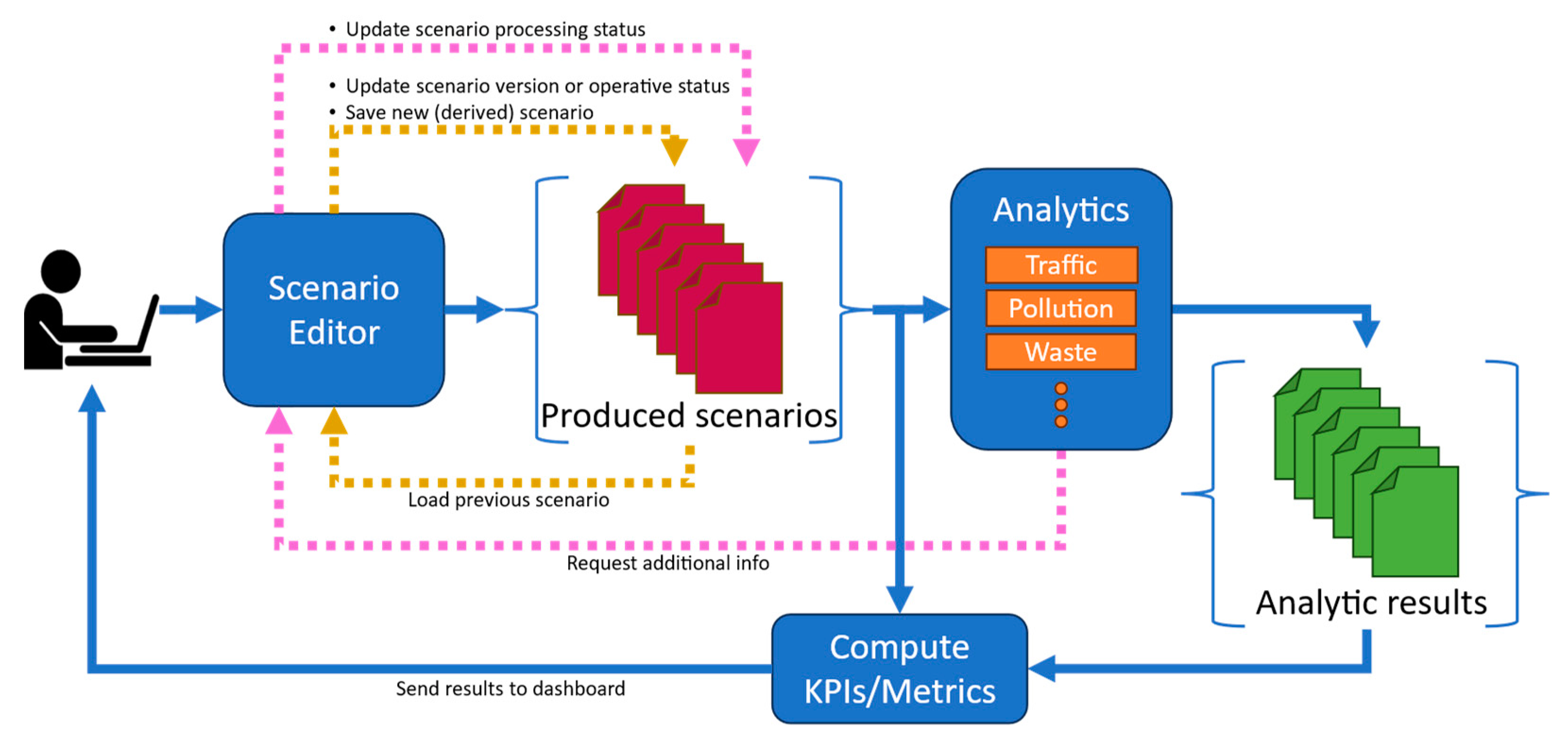
Figure 2.
Snap4City Scenario Editor interface (in edit modality).
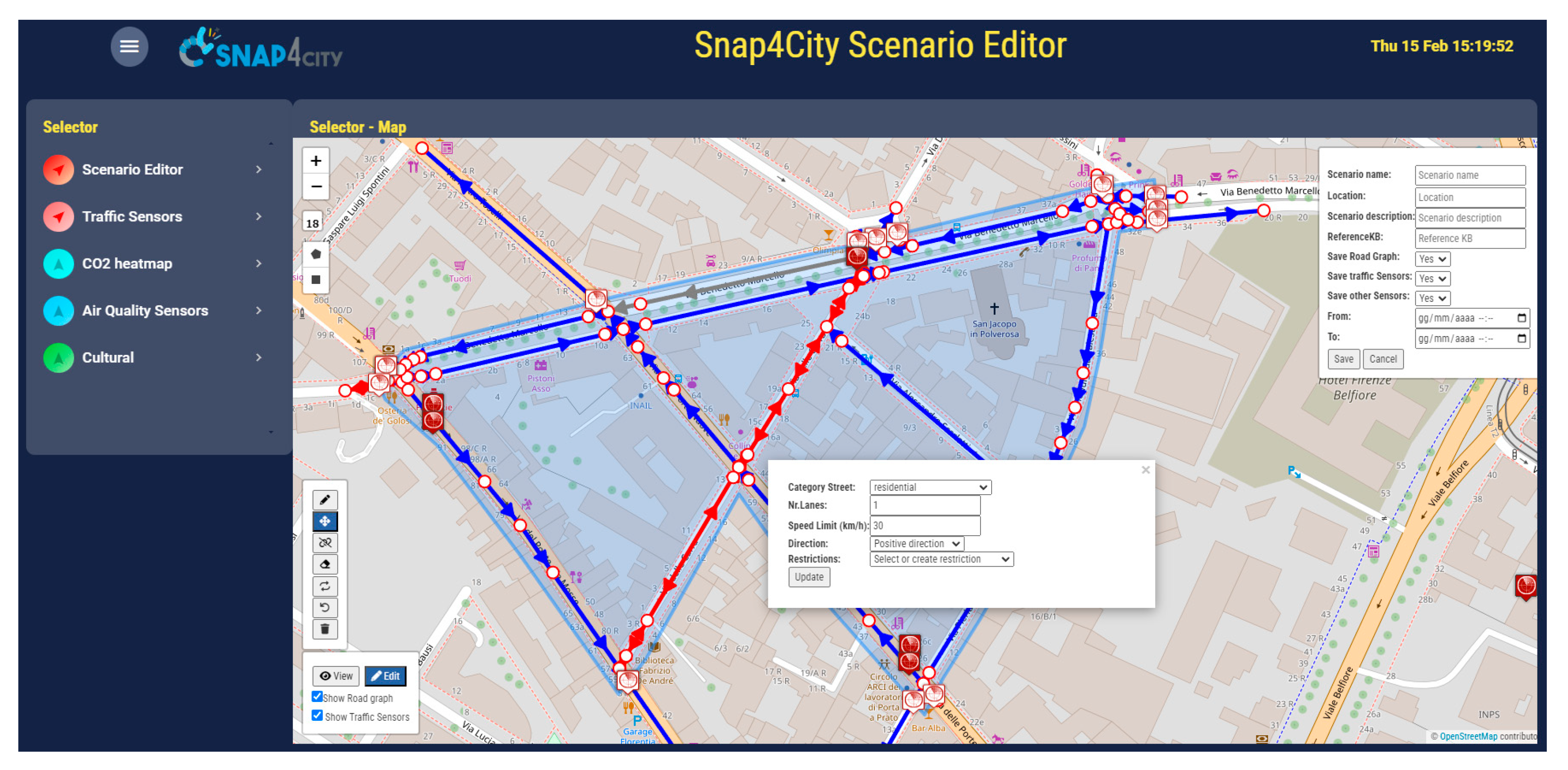
Figure 3.
Consistency test. In (a) the TFR on the whole Florence city macro scale, , the blue rectangle represents the selected area for the comparison. In (b) the specific area delineated using the scenario editor. In (c) the TFR obtained in the micro-scale sub-graph, for the matching segments with . Reconstruction corresponds to 9:00 am on 2023-09-28.
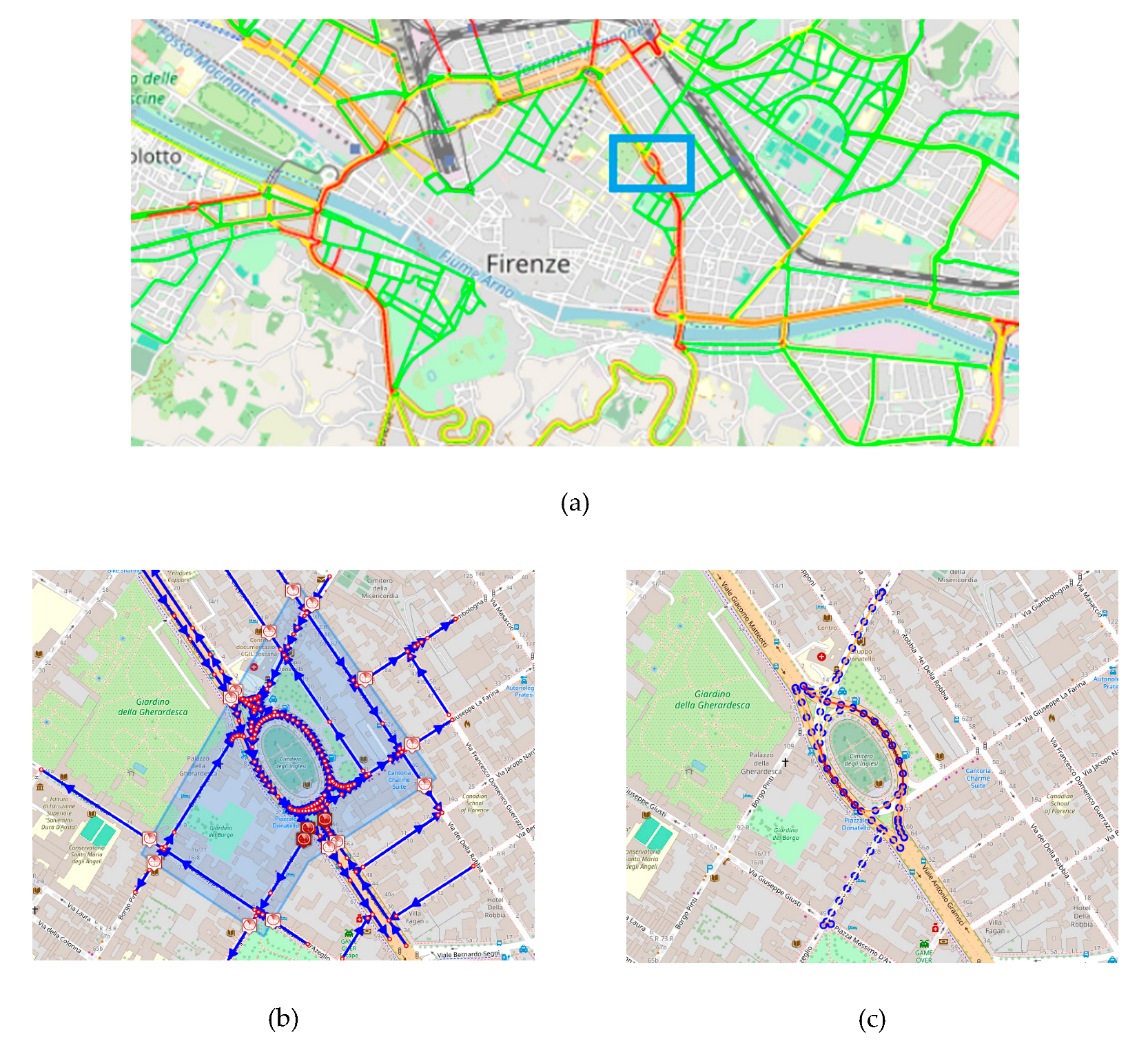
Figure 4.
Consistency test. Comparison of the historical traffic flow reconstruction (red line) and the TFR (blue line) on the 68 segments at 9:00 on 2023-09-28.
Figure 4.
Consistency test. Comparison of the historical traffic flow reconstruction (red line) and the TFR (blue line) on the 68 segments at 9:00 on 2023-09-28.
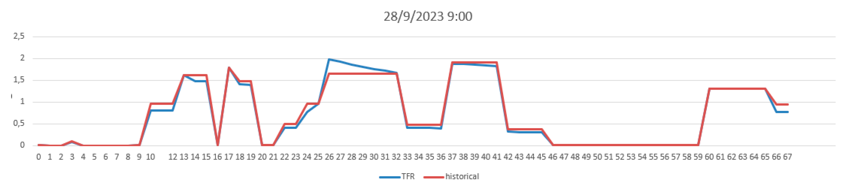
Figure 5.
Graph structure of the road network in the selected area: (a) the graph of ; (b) graph of
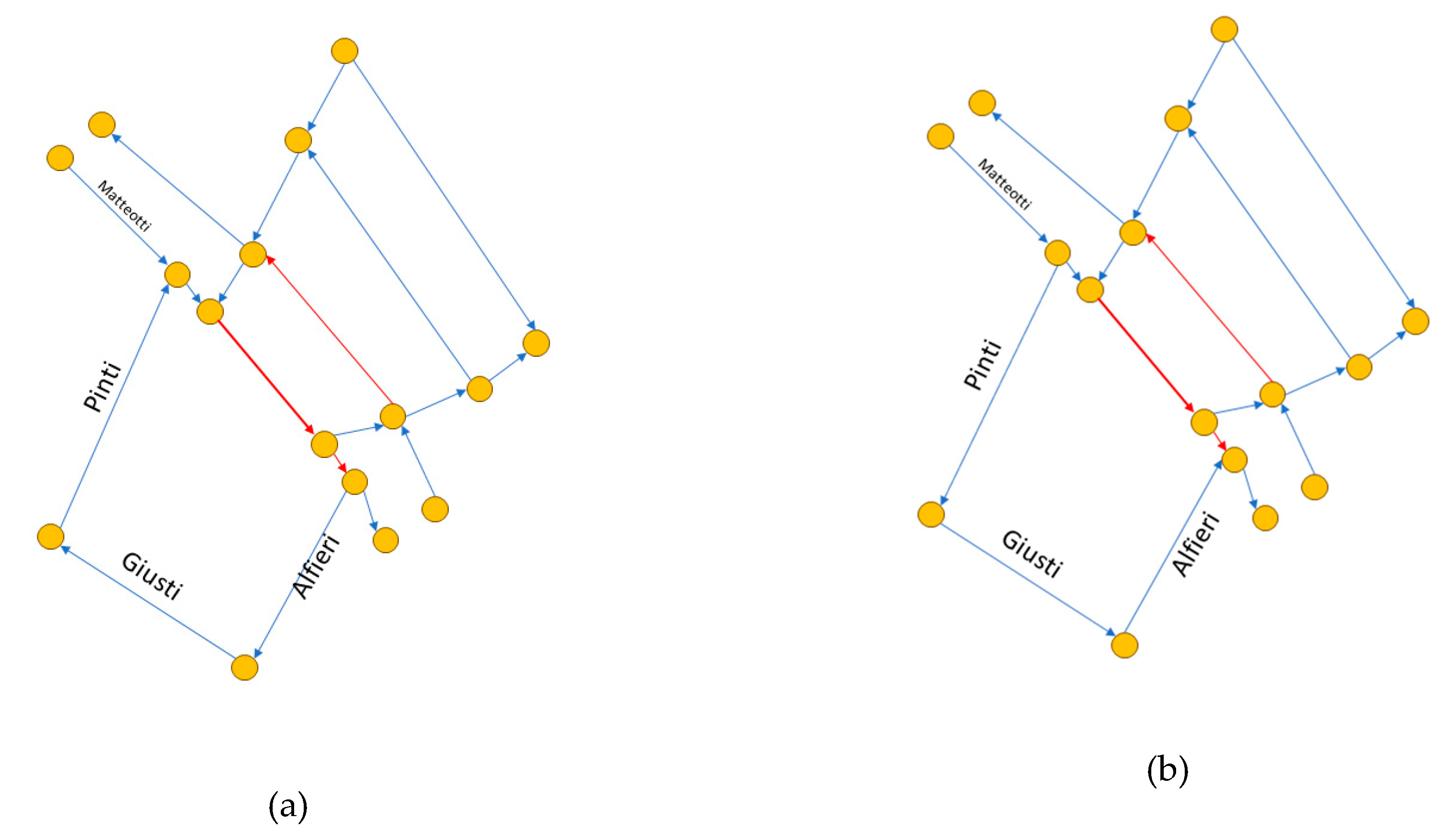
Figure 6.
What-if analysis for TFR. In (a) the current scenario (). In (b) a new scenario with a novel traffic route obtained by inverting the travel direction of three roads (). In (c) the same road network used in but with different TDMs ().
Figure 6.
What-if analysis for TFR. In (a) the current scenario (). In (b) a new scenario with a novel traffic route obtained by inverting the travel direction of three roads (). In (c) the same road network used in but with different TDMs ().
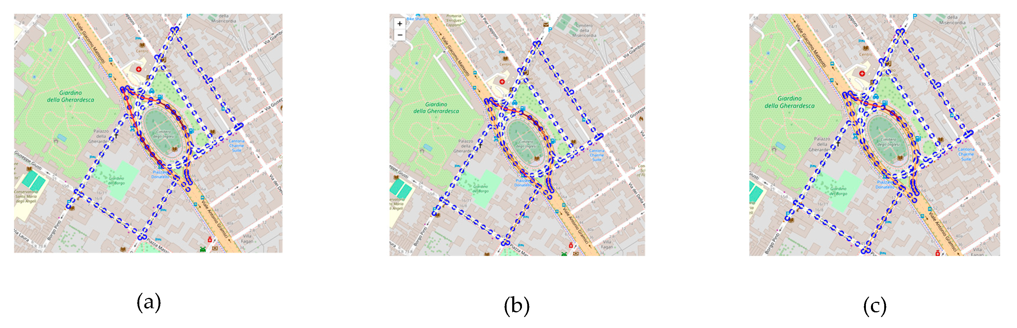
Figure 7.
24 hours TFR comparison in the different segment states FreeFlow (FRrs), FluidFlow (FLrs), HeavyFlow (HErs), VeryHeavyFlow (VHrs).
Figure 7.
24 hours TFR comparison in the different segment states FreeFlow (FRrs), FluidFlow (FLrs), HeavyFlow (HErs), VeryHeavyFlow (VHrs).
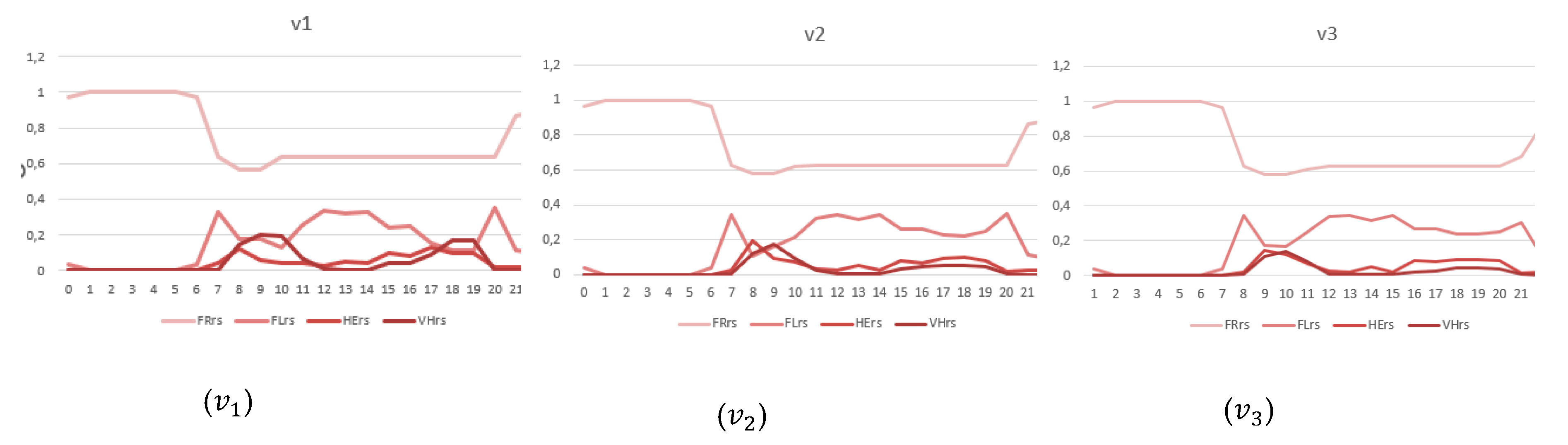

Table 1.
Scenario Editor requirements.
| ID | Name | Description of functionalities of the scenario editor which has to provide support to |
|---|---|---|
| R01 | Map visualization and controls | show/select ground map to be used as the main canvas over which the user can define and study the scenario. Controls to move and zoom the map must be provided, with the possibility of changing the ground map when needed. The map is a visual representation of the geo information, for minimal case, the graphs of roads, their relationships, and details. |
| R02 | Area of interest definition | draw/change a polygonal shape of arbitrary size to define the area of interest of the scenario selecting a portion of the map and of the corresponding geo information. The scenario could be composed of multiple disjoined areas. |
| R03 | Metadata setting | set some metadata describing the scenario, such as its name, a description, the temporal validity (from date time to date time), a responsible, a purpose, etc. |
| R04 | Knowledge base management | work on different maps and geo information, which can be coded into different knowledge bases or other storages from where to fetch the entities and roads of the geo information to be taken into account in the scenario. |
| R05 | Road graph selection and management | manage road graph, and each road segment must be visualized and managed in the scenarios. The road segments may present a number of descriptive characteristics, such as, type, travel direction, presence of restrictions, lanes, sidewalk, parking lots, etc. Each road must be selectable by the user to access to additional information, such as name, type, length, number of lanes, maximum speed, etc. Manipulation of the road graph must be possible, for example to add, remove, or alter a road, invert the travel direction, increase, or reduce the number of lanes, etc. In the representation of road segments visual coding should be used to provide information at a glance. |
| R06 | Entity selection and management | manage geolocated entities as: IoT devices with time series data (such as semaphores, sensors/actuators, waste bins, parking sensors, luminaries, Wi-Fi access points, tv cameras, parking in structures); urban furniture (such as pedestrian crossing, benches, flowerbeds, fountains for drinkable water, toilets); POIs (such as bank, cultural services, schools, commercial areas, restaurants, hotels). They must be visualized over the map on user request. Each entity must be selectable by the user to inspect additional information (i.e., metadata, position, real-time and/or historic data, etc.). Manipulation of entities must be permitted, for example to disable/enable an IoT device, select the measurements of interest, choose between real-time, historic, predicted, typical time trend data, change the semaphore timings, move a pedestrian crossing, etc. |
| R07 | Enabling analytic computation | define the context on which one could apply a large number of analytical processes including for example: computation of traffic flow reconstructions, environmental analysis, environmental heatmaps, 15-minute index, KPI (Key performance indicators) to quantify some analysis, semaphore analysis, etc. For each analytics, the user has to be capable to compose the scenario and compose different inputs. This is the basis to enable the usage of the scenario for what-if analysis, which may use a number of scenarios which are those which have to be inspected to verify their validity for solving a specific case. |
| R08 | Validation by activation of consistency analysis | validate the scenario by means of one or a set of methods to assess its consistency and completeness in terms of road graph, entities, metadata, etc. The validation has to go in deep on the spatial analysis of the road graph as well as the compatibility check among the selected inputs. |
| R09 | Scenario evolution over time | evolve over time in terms of operative status (e.g., proposed, accepted, rejected), processing status (init, runnable, completed) and version. Each step must be related to a specific time stamp. |
| R10 | Scenario management | to create a new scenario, save the defined scenario, load a previously created scenario, and save it again, possibly with a different name, etc. |
| R11 | Models and custom | be conformant to a model, on which additional variables can be added. |
Table 2.
Average flow results on the 24 hours for the three scenario versions for each of the groups FreeFlow, FluidFlow, HeavyFlow, VeryHeavyFlow .
Table 2.
Average flow results on the 24 hours for the three scenario versions for each of the groups FreeFlow, FluidFlow, HeavyFlow, VeryHeavyFlow .
| Scenario Version | FreeFlow | FluidFlow | HeavyFlow | VeryHeavyFlow |
|---|---|---|---|---|
| 0,7649 | 0,1501 | 0.0396 | 0.0455 | |
| 0.7607 | 0.1705 | 0.0414 | 0.0274 | |
| 0.7622 | 0.1744 | 0.0411 | 0.0223 |
Table 3.
Delta values regarding the different traffic states to evaluate the percentage of improvement between the different scenarios.
Table 3.
Delta values regarding the different traffic states to evaluate the percentage of improvement between the different scenarios.
| Delta | Value | Percentage of Improvement |
|---|---|---|
| 0,00416 | -0.54% | |
| 0.00267 | -0.35% | |
| -0.0205 | 13.69% | |
| -0.0244 | 16.27% | |
| -0.0017 | -4.51% | |
| -0.0014 | -3.76% | |
| 0.0181 | 39.86% | |
| 0.0232 | 50.98% | |
Table 4.
Computational times (in seconds).
| Scenario Version | Computational times (s) |
|---|---|
| 161.259 | |
| 162.330 | |
| 159.402 |
Disclaimer/Publisher’s Note: The statements, opinions and data contained in all publications are solely those of the individual author(s) and contributor(s) and not of MDPI and/or the editor(s). MDPI and/or the editor(s) disclaim responsibility for any injury to people or property resulting from any ideas, methods, instructions or products referred to in the content. |
© 2024 by the authors. Licensee MDPI, Basel, Switzerland. This article is an open access article distributed under the terms and conditions of the Creative Commons Attribution (CC BY) license (http://creativecommons.org/licenses/by/4.0/).
Copyright: This open access article is published under a Creative Commons CC BY 4.0 license, which permit the free download, distribution, and reuse, provided that the author and preprint are cited in any reuse.
Submitted:
20 February 2024
Posted:
20 February 2024
You are already at the latest version
Alerts
A peer-reviewed article of this preprint also exists.
Submitted:
20 February 2024
Posted:
20 February 2024
You are already at the latest version
Alerts
Abstract
Nowadays cities, due to the increasing urbanization, are facing challenges spanning on multiple domains as mobility, energy, environment, etc. Big data gathered from legacy systems, from geographic information systems, operators, and Internet of Things technologies can be exploited to provide insights to assess the current status of a city, the possibility to perform what-if analysis to observe the impact of possible changes. The few available solutions for formal scenario definition and analysis are limited to single domain analysis and provide proprietary formats and tools. Therefore, in this paper, we present a novel scenario model and editor integrated into the open-source Snap4City.org platform to define general processing and what-if scenarios in order to carry out analysis on different domains. The proposed solution responds to a series of identified requirements and implements NGSIv2 compliant data models and formal description of the urban context. As a case of study, a traffic congestion analysis is provided, confirming the validity and usefulness of the proposed solution.
Keywords:
Subject: Engineering - Transportation Science and Technology
1. Introduction
Thanks to the increasing deployment of Internet of Things (IoT) technologies and the availability of big data, the concept of smart city is nowadays widely applied worldwide to address current and future challenges in the urban context. Indeed, due to the increasing urbanization, city councils are called to plan and take actions in several domains like mobility [1,2], urban infrastructures [3], energy [4], security [5,6], environment [7], etc. Smart city IoT platforms [8,9] with interactive dashboards [10] and advanced urban digital twin interfaces [11,12] are fundamental tools to assess the current and past states of the cities. However, such technologies should be improved by including solutions for tactic and strategic plans which have to consider predictions and simulations capabilities to help the decision makers in the urban development. In particular, the introduction of what-if analysis solutions [13] to observe the impacts of possible changes to the current urban scenario are required to offer decision makers effective decision support system (DSS) tools. Such solution should provide a structured framework for data-driven decision-making processes leveraging on advanced algorithms and real-time data integration to allow the users to experiment and evaluate the impacts of changes in the urban environment. The first step is to introduce such variations into the representation used to describe smart city entities (roads, buildings, services, green areas, etc.), for example modelled with ontologies or relational databases [14,15]. Therefore, a graphical interface to alter the current representation and formalize a set of hypothetical scenarios, i.e., a scenario editor, according to which assess impacts and effects of city policies in terms of Key Performance Indicators (KPI) and metrics is mandatory.
In the literature, it is possible to find proposals addressing the formalization of scenarios and corresponding editor tools mainly in the context of autonomous driving [16,17], where simulations are carried out to evaluate system response to specific conditions, e.g., complex maneuvers involving multiple vehicles. The formalization of scenario is also useful to decompose the problem for fog and edge computing [18,19]; for shaping context for computation and action [20]; contextualizing and shaping the user behavior [21], etc. A solution could be usage of classic GIS (Geographic Information Systems) tools, e.g., QGIS [22] and ArcGIS [23], in which the definition of shape is possible, and IoT, POI (point of interests), services, and other references may be loaded. However, GIS software tools are typically very far to provide tools for editing the road graph with corresponding semantic information such as priority, lanes, restrictions, velocity, etc., and are far to produce scenario descriptors which can be used for simulation/computation; many other data have to be added. In that context, standards to formalize a scenario emerged, such as the ASAM OpenSCENARIO [24] used in conjunction with the ASAM OpenDRIVE [25] and OpenCRG [26] standards, to describe static and dynamic characteristics. On the other hand, more general tools and models which should be able to cope with a wider concept of city scenarios seem to be less investigated. Some solutions with specific capabilities have been proposed as commercial or open-source software. For example, the OpenStreetMap (OSM) ecosystem provides the iD editor [27], a web-based editor to modify OSM map elements in an intuitive manner. However, the introduced changes are directly incorporated into the OSM database, limiting the possibility of producing multiple scenarios to be analyzed simultaneously at the basis of computation and machine learning (ML) or artificial intelligence (AI) solutions/simulation. In addition, the area of interest of the OSM scenario is not formally defined to be directly exploited for successive computations and/or simulations and need to be extracted by means of complex SQL queries. More advanced models and tools are proposed by SUMO [28], and PTV for Vissim [29] and Visum [30] simulators. SUMO is an open-source traffic simulator and includes as scenario editor the so-called SUMO netedit tool [31]. It allows to add, modify, and remove roads and connections as well as change the element attributes, such as number of lanes, speed limits, etc. Different file formats are accepted as input and output, including the OpenDRIVE standard. PTV Vissim and Visum are two proprietary simulators, for micro and macro scales, respectively. Both solutions include a similar editor where the user can define changes to the current scenario by altering the road network. However, both SUMO and PTV editor requires on-premises installation, while a web-based interface would be preferable for easiest access and wider distribution. Moreover, none of the available solution can automatically extract and integrate information coming from IoT sensors time series, an important source typically available in smart city environments, that can be used to extend the focus of the simulation from the traffic to other problems like pollution, waste management, index computation, etc.
In this paper, the development of a model for scenarios and corresponding web based open-source tool for scenario editing are presented. To this end, a collection of requirements has been identified and reported. From the scenario editor, the user can select an area of interest and modify the topology and the attributes of the road network. Then, different kind of IoT devices, entities, and services can be recalled and selected n order to complete the formalization of the scenario for computing and analysis phases. The aim was the definition of a powerful scenario model and tool which can be used to define the context for a huge number of context-depended computational activities (in time and space) such as those for computing people flows, traffic flow reconstructions, heatmaps, origin destination matrices, indicators, navigation, representation, etc., maybe extracting information from multiple big data spaces, knowledge bases/graphs, etc., and allowing the users to produce also hypothetical scenarios/contexts on which the computation/simulation could be performed, as in the what-if analysis. The formalization of scenarios in a flexible manner enables the assessment of the impact of changes in complex city contexts. The modeling of the scenario itself could change its status (e.g., proposed, approved, closed), evolving over time, and be shared among experts and decision makers. In the proposed scenario management, the model definition and structure is formalized as a smart data model compatible with the NGSIv2 standard for data exchange and indexed into a knowledge base for future retrieval via semantic queries [14]. In this paper, the requirements and the formalization of the scenario and editor are presented. In addition, a case study is provided in which the scenario model and tool are used to define the context and needed to compute the traffic flow reconstruction of a portion of the city, in actual conditions and by changing some constraints enabling in this case the fast re-computation/simulation for what-if analysis. The proposed scenario model and editor have been developed and are integrated into the Snap4City platform (https://www.snap4city.org/), an open-source IoT platform able to manage multiple tenants and billions of data with the key focus on interoperability (the tool is accessible from dashboards such as [32]). The scenario editor is embedded as a novel module of Dashboard Builder Multi Data Map widget [33] and is able to retrieve static (road graph, urban elements, sensor positions, etc.) and real-time (sensor readings, public transport time schedules, weather, temperature, etc.) data though specific APIs.
The main contributions of this paper are:
- The definition of a series of requirements that a scenario editor must meet;
- The definition of the smart data model describing a scenario and a formal model to describe the road network;
- The development of an open-source web-based scenario editor, and its integration into the Snap4City platform;
- A case study to show the scenario editor functionalities applied to the traffic flow reconstruction problem, to validate the scenario model and tool.
This paper is organized as follows. In Section 2, the general architecture and data flow related to the scenario model and editor is presented. In Section 3, the requirements defined to guide the development of the scenario model and editor are provided, together with the formal definition of a scenario as a smart data model. In Section 4, the Scenario Editor is described. Section 5 presents a case of study where the scenario model and editor is used to perform traffic flow reconstruction and congestion analysis for what-if analysis. Finally, in Section 6 conclusions are drawn. This research has been performed in the context of MOST National Center on Sustainable Mobility in Italy [34], Snap4City is one of the reference platforms for the CN MOST.
2. Context definition
Figure 1 depicts a conceptual block diagram describing the workflow for scenario production and evaluation, therefore defining the operative context for the scenario editor. As can be seen, the user interacts with the scenario editor interface by specifying the area of interest, datetime, metadata, loading and selecting real or simulated data (sensors, services), etc., and may be altering the current scenario in all details. All the data are retrieved from Snap4City storage by performing queries on Km4City knowledge base or any other storage. The produced scenario, with or without modifications, with respect to a current condition, may be saved, exported/imported, shared according to a smart data model (see Section 3.1) and can be readily used as input to compute KPIs and metrics, as, for example, the evaluation of heatmaps on the basis of sensors data into the scenario, or computing a 15-minute city index [35]. The same or multiple scenarios can be used in input to one or more data analytic processes to compute traffic flow reconstructions, pollutant predictions, people flows, simulations such as the traffic flow reconstruction [36], the computation of heatmaps [37], the management of waste [38], etc. Analytic results are then passed to the KPI and metric computations to quantify the impact of the produced scenarios, to compare the value of those KPI/metrics in the current situation with respect to the modified scenario according to the changes as in What-if analysis. Finally, obtained results and comparison are shown to the user.
Note that, the scenario editor can take as input a previously created scenario (see yellow arrows in Figure 1) that the user can further modify to obtain a novel version of the same scenario, create a new scenario derived from the old one, or change the operative status of the scenario, e.g., from proposed to approved or rejected status. This approach opens the path for collaborative work on what-if analysis, city development and study [39,40].
Moreover, some analytics can require additional information (pink arrows in Figure 1). In this case the scenario is presented again to the user that specifies the missing information and change the processing status of the scenario, e.g., from init to under analysis. Using the scenario versioning and status is possible to save and track the history/evolution of a scenario model and reduce the work of the users. To give the reader an example, let us now to suppose that due to scheduled street works some roads should be closed to traffic and the city council must find the best solution to avoid congestions. The mobility operator of the city has to assess the impact and find a solution, he/she starts by creating a first scenario, , by closing some roads to traffic to study what happen if those changes are performed. Then, is loaded into the editor and the user adds further changes, such as inverting some road travel directions, creating a scenario . The operator loads again and this time changes the number of lanes of some roads to create the scenario .and are derived scenarios from and both have version set to v0 and operating status to proposed. and are sent to the traffic flow reconstruction to assess which is the better solution to limit traffic congestion due to the closed roads. The city chief of the mobility operators decides is not a valid solution: the operative status of passes to rejected. At the same time, the city council requires further changes to that the user implements, updating the version of to v1. After a second round of reconstruction and computation of KPIs, is accepted and its operative status moves to approved. Thus, the formal definition of robust model for scenarios is the first step to create also automated models and tool to AI based tools for automated generation of best scenarios which in any case have to be verified and selected from the mobility city chief.
3. Requirement Analysis and Scenario Data Model Definition
In this Section, the identified functional and non-function requirements for the development of the Scenario Editor are presented and discussed. Functional requirements are reported in Table 1, with ID, name, and a brief description, while non-functional requirements are discussed in the following.
As can be seen in Table 1, eleven functional requirements have been defined. Since scenario editing is performed on geographical areas, a ground map and associated controls are required (R01). Requirements from R02 to R04 are needed to define the specific context for the scenario. These include the drawing of the area of interest, the description of metadata, the selection of the knowledge base or storages from where to fetch the data. Requirements R05 and R06 describes the main viewing and editing functionality available to the user, from the selection of the data to consider, to their manipulation in order to define alterations of the current scenario. Note that, according to R07, a scenario editor must allow to load (and modify) heterogeneous data so as to be exploitable with multiple analytics and KPIs to perform different kinds of what-if analyses. Since the editor allows the operators alter entities and roads as well as select different areas, a check of consistency (R08) should be carried out to avoid the creation of unrealistic scenario: for example, unreachable road segments due to wrong travel direction assignments. There should be the possibility of creating scenarios with different statuses and versions (R09): a processing status progression could be required by specific analytics, requiring user intervention on different steps of the process. On the other hand, the scenario operative status and version could be used to describe the evolution of the scenario and track the introduced changes, may be revert. Therefore, the scenario editor should provide the possibility to create and save the scenario, and to load a previously defined scenario (for example to define a new version or to advance the scenario status) and save it with a new name (R10). Finally, the scenario editor must produce a scenario conformant to a given model that should be sufficiently elastic to accommodate additional variables (R11).
Some non-functional requirements must also be defined. At first, the editor should be implemented as a web application, to avoid the need for installing software and guarantee a wide accessibility and coworking. High level of performance should be achieved both in terms of quick response times to offer a seamless interactivity, high reliability, and availability to avoid service interruption. Security and privacy aspects must also be considered: this requires the implementation of adequate management of user profiles with different roles and with different organizations to which any user can be associated with. Moreover, the possibility to delegate or make public the access to data, defined scenarios, or analysis results is required to enable multiple users to work on the same problem in a collaborative way. For example, an operator could prepare different scenarios and results and then delegate/share them to the office manager/chief who takes the final decision.
To satisfy all the non-functional requirements and some of the functional ones (R01, R04, R05, R06, R07) the proposed scenario editor has been integrated into the open-source IoT platform Snap4City. The platform includes functionalities to collect data from different sources though push and pull modalities using brokers, gateways, and services, and to index them in the Km4City knowledge base [14], and shadow store the data in an OpenSearch cluster. Using specific APIs, data can be retrieved using spatial, temporal, and relational queries, therefore addressing R04, R05, and R06. Multiple analytical methods (R07) are available as well as solutions to compute KPIs based on Node-RED flows according to national and international specifications like the SUMP [41], Italian PUMS [42] and European SUMI [43]. Moreover, Snap4City is GDPR [44] compliant and successfully passed several penetration tests, uses multiple user’s roles, handles different organizations, implements data and service ownership functionalities with the possibility to change ownership, delegate, or make the resources available for given organizations or to the public. The main installation uses up-to-date redundancy solutions to guarantee a high level of reliability. The proposed scenario editor is integrated as an extension of the multi data map of the DashboardBuilder to create a map widget with navigation controls (R01) and can be included in any Snap4City dashboard and accessed with any web browser.
3.1. Scenario data model
Hereafter a formal definition of the data model for a smart city scenario is provided, responding to requirement R11. Such definition was developed to store the needed data and information according to the functional requirements presented in the previous section. A scenario is described as a context entity compliant with the FIWARE NGSIv2 specification [45], with a type SmartCityScenario and an ID defined as an URI, corresponding to an entity instance in the knowledge base. A scenario has the following attributes (with data types reported in brackets):
- A1.
- name (string): the name of the scenario;
- A2.
- description (string): a brief description of the scenario;
- A3.
- location (string): the textual name of the geographic area considered;
- A4.
- startDatetime (string): timestamp of the starting instant from which the scenario is valid, represented as ISO string;
- A5.
- endDatetimes (string): timestamp of the last time instant for which the scenario is valid, represented as ISO string;
- A6.
- areaOfInterest (geometry): a polygon describing the portion of the city over which the scenario is defined, represented as GeoJSON;
- A7.
- knowledgeBase (string): the ID of the knowledge base used to fetch the data in the scenario, represented as URI. It also identifies an Organization or tenant in the multitenant Snap4City platform
- A8.
- entities (data structure): IoT devices or other urban entities (e.g., traffic sensors, semaphores, POIs, buildings, gardens, waste bins, etc.) considered in the scenario and included in the area of interest, represented as JSON. Each entity is identified with an URI associated to an instance in the knowledge base;
- A9.
- roads (geometry): a list of roads included in the area of interest, represented as a GeoJSON, according to the formal model described in Section 3.2. Each road is identified with an URI associated with an instance in the knowledge base;
- A10.
- restrictions (data structure): a list of traffic or access restrictions applied to entities and roads of the scenario, represented as JSON;
- A11.
- additionalData (data structure): data required by specific analytics, represented as JSON;
- A12.
- processingStatus (data structure): a list indicating the status of the scenario for each used analytic, represented as a JSON. Each list entry can assume different values depending on the analytic to which it is referred;
- A13.
- operativeStatus (string): a description indicating the status of the scenario; it can assume the following values: proposed, approved, rejected;
- A14.
- version (string): the version of the scenario, used to implement a versioning system. Please note that an automated versioning approach based on time is implemented by using dateObserved attribute;
- A15.
- dataObserved (string): timestamps of the creation/ modifications of the scenario, represented as ISO string.
Attributes A1 – A5 describe the metadata of the scenario, responding to requirement R03. A6 is used to store the area of interest (R02), while in A7 the URI of the reference knowledge base is set (R04). To satisfy R05 and R06, attributes A8, A9, and A10 are used to store respectively the entities, the roads, and the restrictions included in the scenario and possibly modified. R07 and R11 are addressed with attribute A11, used to store possible additional data required by analytics or KPIs. A12 is used to track the processing steps reached with some analytics. Finally, A13, A14, and A15 are related to requirements R09 and R10 to take into account different operative statuses and versions.
In order to respond to requirement R08, in the next section, a formal method to assess the validity of the (possibly modified) road graph included in a scenario is presented.
3.2 Formal road graph data model
In this section, the formal representation of the road graph of the scenario model is presented in order to: facilitate reasoning and formal verifications over the road graph, as well as to provide a formal framework to define KPIs involving the road graph and data connected via knowledge base.
Full Road Graph definition. The full road graph (FRG) is defined as a tuple
where:
- is the set of nodes forming the road graph (i.e. the road junctions);
- is the set of edges of the road graph, where means that there is a physical link allowing to go from node v to node w and vice versa,
- R is the set of roads,
- is a function associating a GPS position to each node,
- is a function associating to each edge the road it belongs to,
- is a function stating for each edge the direction it can be traversed, means it can be traversed in both ways, only from to , only from to ;
- is a function associating for each edge the number of lanes (>0),
- is a function to associate each edge with its max speed.
- models turn restrictions where tuple means that the restriction of type applies to the edge via the node to edge , the node has to be shared between edges and , for example restriction means that from edge it is not possible to turn to edge .
The FRG is used to represent all the detailed road shapes, and from this it can be built the Compact Road Graph (CRG) where edges connected in a sequence having the same associated data (dir, road, lanes, max_speed) can be represented as a single edge. For this purpose, we introduced the following functions:
where eq. (2) returns the set of edges that are insisting on edge , while eq. (3) gives the set of edges that are next to . Symbol is a projection function used to get the i-th component of a tuple/sequence, i.e., and provides the last element of a sequence. Function on a sequence provides the subsequence without the last element.
Compact Road Graph definition. Given a FRG as in eq. (1) its compact version (CRG), is expressed as
And it can be built by introducing an additional mapping function that maps each edge of the compact version to a sequence of edges of the full version. With the following constraints:
- , the set of nodes of the compact version are a subset of the full version,
-
and
- maps to the longest possible sequence of edges
Whether, in the compact graph, there exist edges having only one next edge, i.e., , means that there exists an edge on the road where the direction or the number of lanes or the max speed or the road name are changing.
Note that, with respect to a naïve graph modelling of the road network, the FRG or the CRG representations are required in order to take into account the possible restrictions. Then, in order to assess, if a road graph (full or compact) is meaningful, some standard graph algorithms can be used to check for example the number of connected components or to find the shortest path between two nodes since in a well-designed road network all nodes should be reachable from all the other nodes.
4. Scenario Editor
The Scenario Editor was developed and enforced in Snap4City tools according to the requirements presented in Section 3, with the aim of providing a versatile and easy-to-use operator tool for defining, studying, and analyzing smart city scenarios [32]. In Figure 2, a screenshot of a Snap4City dashboard including the proposed scenario editor is provided. As can be seen, a map is used as background while on the left and right sides of the map are placed panels and buttons that can be used to create the scenario. The save functionality is accessible on to registered users, and the registration is free of charge.
The editor can work in edit and view modalities (see the button in the bottom-left corner of the map): the former is the modality to define a scenario and introduce changes, the latter is used to display previously created scenarios, received in delegation of made public. On the right side, a panel to specify scenario metadata is displayed, including fields for the scenario name, location, description, reference knowledge base, analytics and KPI to use, start and end datetimes of the scenario validity. In the top-left corner, under the buttons to set the map zoom level, controls to draw a squared or polygonal shape are provided. After having defined the shape of the area of interest, the road graph is retrieved from the specified knowledge base and shown over the map with interactive graphical elements. Roads are displayed with arrows specifying the travel direction and with different color to indicate if roads are not in use (gray, not to be considered in the scenario processing), if they are with a single (blue) or double (red) travel direction. Each road segment can be clicked to access and modify specific information (category, number of lanes, max speed, etc.). Using the button in the bottom-left corner, roads can be modified by creating, splitting, or deleting segments, dragging and joining nodes. Undo and redo actions are implemented to help the user in correcting possible errors. Entities are requested using the selector menu on the left side of the dashboard. Each selector entry specifies an entity kind (traffic, weather, air quality sensors, POIs, bus stops, etc.) that can be loaded independently into the scenario editor. Once the user completes the editing operations, the resulting scenario can be saved using the format described in Section 3.1.
Before saving the scenario, the system performs a consistency check on the defined road graph to highlight possible errors using the formal method described in Section 3.2. In the case the consistency check fails -- e.g., when nodes with only entering roads are detected, an alert is sent to the user and the different components are highlighted in the map. Additionally, a warning is given to the user when the system detects roads having segments with different number of lanes or different max speeds. Even if, this is something that may happen in real cases, due to the relevance of such characteristics, the system highlights suspicious cases to help the user avoiding introducing errors in the scenario.
In the next section, as case study, about the usage of the scenario editor for traffic flow reconstruction and what-if analysis is presented.
5. Case of Study: Traffic Flow Reconstruction
Understanding the evolution of traffic within urban environments is important for effective city planning and management to face the challenges posed by growing populations and increasing vehicular density, or to address events and planned activities on the urban infrastructure. Accurate insights into how traffic patterns evolve over time enable decision-makers to implement strategic measures that enhance mobility, reduce congestion, and improve overall urban resilience. In this context, the traffic flow reconstruction case study presents a comprehensive approach, utilizing the scenario editor and data-driven tools to analyze and reconstruct traffic flow in the area of interest, performing what-if analysis, and therefore contributing to informed decision-making.
The proposed scenario editor is used to select a specific area of the map, retrieve information about the road network and traffic sensors, and possibly to apply changes, defining a new scenario for traffic analysis. The scenario editor allows the users to choose which sensors take into account for the traffic reconstruction procedure, or to assign some reference time trends. Traffic flow reconstruction (TFR) is carried out exploiting the algorithm presented in [36] that is based on the solution of a fluid dynamic problem based on partial differential equations (PDEs). As usual in PDE problem solutions, boundary conditions must be specified: in this case the reconstruction method requires to know the traffic flow entering the area of interest. For this reason, the scenario editor automatically detects road sections that intersect the area of interest and whose direction is entering in the area. On these points virtual traffic sensors are placed, in which the user can specify 24 hours trends to be used as input. Different kinds of traffic time trends can also be exploited, as for example typical time trends generated from historical traffic data, predicted typical time trend data, or arbitrary time trends defined by the user. Once completed the editing process, the scenario is saved according to the defined data model (see Section 3.1), with the scenario processing status attribute set to init. Then, the user can load the scenario in the TFR analytic, and a first pre-processing phase can be carried out: road intersections connected to only two road segments with same number of lanes and max speed are removed and the related road segment merged, passing from a FRG to a CRG (see Section 3.2). This reduces the fragmentation of the road network, helping in the required discretization of the numerical solution (see [36] for further details). After this phase the scenario is updated: attribute A9 now describe the CRG, and the processing status moves to merged. Then, additional inputs are requested from the user. The scenario is loaded into the editor, and the user is asked to set the road segment capabilities (i.e., an estimate of the number of vehicles that a road can accommodate). Such information is exploited to compute the so-called Traffic Distribution Matrices (TDM) that represent how vehicles are distributed at road junctions. More precisely, so that and , for and , where coefficients (called weights) are the percentages of vehicles arriving from the -th incoming road and taking the -th outcoming road (assuming that, on each junction, the incoming flux coincides with the outcoming flux). The scenario is saved again, with road capabilities and TDM saved in the additionalData attribute (A11), and the processing status set to ready. Now the TFR can run on the updated scenario to compute the traffic reconstruction.
To assess the correctness and the validity of the proposed approach, two tests were carried out. At first, we study the correspondence between a TFR computed on a wide road network, i.e., the whole city of Florence (Italy), and the reconstruction obtained on a small sub-graph, i.e., the scenario area of interest, to evaluate traffic flow discrepancy (see Section 5.1). Then, in a second test we assessed the impact of alterations in the road graph by changing road travel directions to create additional paths with the objective of reducing congestion on the principal roads (see Section 5.2).
5.1. Consistency and correctness of TFR
A first assessment analysis has been performed to assess the correctness of the TFR. A small area of the city of Florence (see Figure 3a) has been selected to test if the TFR results are consistent with the one extrapolated by the traffic flow reconstruction computed on [36] in the small/micro-scale scenario. The historical traffic flow reconstruction computed in the 28th September 2023, referred as , has been chosen for the analysis.
Using the scenario editor, the area of interest has been selected (see Figure 3b). On the area of interest, the scenario provides the road elements on which the historical reconstruction was performed. The virtual sensors were considered to reproduce the same boundary conditions and they have been initialized with flow values of for the considered road segments, inside the area. The traffic sensors inside the scenario have also been considered and the same TDMs has been imposed to obtain the small-scale reconstruction for the defined scenario, referred as . The reconstruction at 9:00 am on 2023-09-28 is reported in Figure 3c.
The TFR algorithm produced almost identical traffic flow reconstruction results on the defined micro-scale scenario with respect to the macro scale, showing an equal level of congestion on the corresponding road elements. In Figure 4 is reported the charts with the historical traffic flow reconstruction values and the TFR at 9:00 on 2023-09-28 where 68 road segments of 20m are compared. The reconstructions show a high degree of correspondence. In average, a mean absolute error of 0.05648 (cars/20m) was achieved, demonstrating the robustness of the TFR method and the validity of the proposed approach passing from macro to micro scale computation. The mean historical value for reference was 0.734774 (cars/20m) and the error performed is about 6.81%. Note that, we could not achieve perfectly identical results since in the selected sub-graph generated a different merged graph with respect to , and, as consequence, the reconstructions worked on slightly different road segments in length, preventing a perfect match between and road graphs.
5.2. What-If analysis for traffic congestion reduction
In this second test, we exploited the scenario editor to perform what-if analysis on traffic flows. The chosen area is the same on which has been performed the consistency and correctness analysis and is reported in Figure 3b, referred as version whose graph structure is reported in Figure 5. This area is often congested in the main roundabout and in Figure 5 this road sections are highlighted in red. Measurements for real traffic sensors encompassed in the area, and for the virtual sensors on the border were sampled from historical data. No changes were introduced in the road network.
With the aim of improving the traffic flow in the selected area using the editor, it has been possible to study an alternative road network configuration, version , by inverting the travel directions for streets: Borgo Pinti, via Giuseppe Giusti, and via Vittorio Alfieri. The new path should alleviate the traffic flow moving from north to south, redirecting a part of the traffic on alternative path. The graph structure of is also reported in Figure 5. The value related to TDM estimation of Matteotti was set to 70, and the Pinti one to 12. This means that in percentage 14.63% or cars should take Pinti as route and the remaining 85.36% should continue on the roundabout, according to the weight coefficient in the TDM. To complete the possible scenario versions another one has been considered taking and changing the value of Pinti from 12 to 25 in the TDM. Meaning that: what if more cars would choose that route? In detail, what would happen if instead of around 15% the percentage of vehicles choosing Pinti was in this case 26.32% increasing of about 10%.
According to What-If analysis, we tested if the new configuration could improve the traffic jam in the selected area, it has been performed the TFR for , , whose reconstructions are reported in Figure 6. As can be seen, by having created a new route, the congestion on the main road decrease with respect to . However, from the graphs in Figure 6 it is possible to note that in there is still a 20m segment in heavy traffic flow state (represented in red), meanwhile in no congestion is visible on the main road.
To quantify the improvements, we divided the road segments in four groups, depending on the measured traffic density in the initial scenario w.r.t. the critical density (equal to half the maximum density, i.e. ): FreeFlow, if ; FluidFlow, if ; HeavyFlow, if ; VeryHeavyFlow, if . Note that, traffic flow and density are related with the following equation:
where is the maximum velocity.
In Figure 7, the traffic density for the 24 hours in the four groups for , , are reported. The trends reveal the decrease of the number of road segments in the Very Heavy traffic status from to and . However, the differences between and are less evident from the trend graph. The results have also been reported numerically in Table 2 that contains the average values (h24) for the different states in the different versions of the scenario considered. The major improvement can be seen in the percentage of segments in the Fluid Flow state with respect to and , rising from to 0.1501 to 0.1705 and 0.1744 respectively. Even if the percentage of segments in the Heavy Flow state slightly increases in the modified versions this is acceptable since it determines an important decrease in the segments in the Very Heavy Flow from 0.0455 in to 0.0274 of and 0.0223 in .
To evaluate the overall improvement in the traffic in the defined scenarios specific delta metrics for the different traffic density states have been defined as follows:
- ,
- ,
- ,
Please note that, if and are positive, then the number of segments (in percentage) having uncongested traffic states decrease passing from the original scenario to the modified one. Generally, the occurrence of a positive value in (and assumes a negative effect. Thus, when and are negative values, the traffic state is improved between the compared scenarios. This means that, the uncongested traffic state increases passing from the original scenario to the modified one. Vice-versa, if and are positive, then the uncongested traffic state decreases during the scenarios’ comparison.
In order to evaluate the percentage of improvement according to FreeFlow, FluidFlow, HeavyFlow, VeryHeavyFlow traffic states, we have to consider a multiplicative contribution factor according to the above dissertation. Then, -1 in cases of FRrs and FLrs estimations, while 1 when HErs and VHer are considered. For example, in order to estimate the percentage of improvement of the scenario with respect to the original one, we consider the following formula for FRrs, where -1:
Similarly, different states are evaluated, and the related estimation is reported in Table 3. The results demonstrate that, with respect to scenarios , and reduced the proportion of segment in the VeriHeavyFlow state of 39.86% and 50.98% respectively, and at the same time, augment percentage of segments in the FluidFlow class by 13.69% and 16.27% respectively. On the other hand, the segments in the FreeFlow status reduce, and those in HeavyFlow augment. However, such negative impact is very slightly compared to the benefits obtained, that significantly reduce the overall congestion, in particular on the main roads.
Finally, in Table 4 the execution times for the three scenarios are reported. Computations have been carried out on a workstation equipped with an Intel i7 CPU, with 32 GB of RAM. No GPU was used. As can be seen the TFR computation for 24h results is around 160 seconds with a slight difference between the three versions.
6. Conclusions
In this paper a novel scenario model and editor have been presented. The solution has been designed according to a large range of smart city requirements analysis for covering relevant cases in computing scenario based: metrics, KPI, heatmaps, traffic flow, etc. The editor, responding to a series of requirements and implementing standard data models and formal method analysis, allows the user to load and visualize the road network and other entities in a specific area and give the possibility to alter the current status to define multiple what-if scenarios. A case study has been presented, involving the production of a scenario for traffic congestion analysis showing how the proposed solution could be effectively used to realize a decision support system to help city councils and decision makers to answer the current and future necessities of a smart city. The formalization of the scenario allowed to pass from macro to micro scale computation without losing of generality for the traffic flow. Thus, analytic software, already implemented and accessible in the Snap4City open-source platform, can be used to carry out predictions, simulations, and reconstructions to assess the impact of changes in different domains (e.g., mobility, energy, environment) in terms of different possible KPIs and metrics. The scenario editor is accessible and can be tested on Snap4City.org. It is presently in use on the research and development activities of the CN MOST in Italy. CN MOST is the national Center on Sustainable Mobility in Italy.
Author Contributions
Conceptualization, P.N.; methodology, P.B., S.B., M.F. and P.N; software, L.A., D.B. and E.C.; validation, S.B., D.B., E.C., M.F. and P.N; formal analysis, P.B., S.B., M.F. and P.N; investigation, S.B., E.C., M.F. and P.N.; data curation, P.B. and M.F.; writing—original draft preparation, P.B., S.B., E.C., M.F. and P.N.; writing—review and editing, M.F. and P.N.; visualization, E.C. and M.F.; supervision, S.B., M.F. and P.N.; project administration, P.B., M.F. and P.N.; funding acquisition, P.N. All authors have read and agreed to the published version of the manuscript.
Funding
This research was financed by the European Union—NextGenerationEU (National Sustainable Mobility Center CN00000023, Italian Ministry of University and Research Decree n. 1033— 17/06/2022, Spoke 9).
Institutional Review Board Statement
Not applicable.
Informed Consent Statement
Not applicable.
Data Availability Statement
Not applicable.
Acknowledgments
The authors would like to express a sincere thanks to the MIUR, CN MOST. A special thanks to the many developers working on the Snap4City platforms. Snap4City (https://www.snap4city.org, accessed 31 January 2024) and Km4City are open technologies of the DISIT Lab.
Conflicts of Interest
No conflicts of interest are involved among the authors.
References
- Torre-Bastida, A. I., Del Ser, J., Laña, I., Ilardia, M., Bilbao, M. N., & Campos-Cordobés, S. (2018). Big Data for transportation and mobility: recent advances, trends and challenges. IET Intelligent Transport Systems, 12(8), 742-755. [CrossRef]
- Bellini, P., Bilotta, S., Collini, E., Fanfani, M., & Nesi, P. (2024). Data Sources and Models for Integrated Mobility and Transport Solutions. Sensors, 24(2), 441. 2. [CrossRef]
- Hodson, M., Marvin, S., Robinson, B., & Swilling, M. (2012). Reshaping urban infrastructure: Material flow analysis and transitions analysis in an urban context. Journal of Industrial Ecology, 16(6), 789-800. [CrossRef]
- Keirstead, J., Jennings, M., & Sivakumar, A. (2012). A review of urban energy system models: Approaches, challenges and opportunities. Renewable and Sustainable Energy Reviews, 16(6), 3847-3866. [CrossRef]
- Gharaibeh, A., Salahuddin, M. A., Hussini, S. J., Khreishah, A., Khalil, I., Guizani, M., & Al-Fuqaha, A. (2017). Smart cities: A survey on data management, security, and enabling technologies. IEEE Communications Surveys & Tutorials, 19(4), 2456-2501. [CrossRef]
- Collini, E., Palesi, L. A. I., Nesi, P., Pantaleo, G., & Zhao, W. (2023). Flexible thermal camera solution for Smart city people detection and counting. Multimedia Tools and Applications, 1-29. [CrossRef]
- Charnes, A., Cooper, W. W., & Li, S. (1989). Using data envelopment analysis to evaluate efficiency in the economic performance of Chinese cities. Socio-Economic Planning Sciences, 23(6), 325-344. [CrossRef]
- C. Garau, P. Nesi, I. Paoli, M. Paolucci, P. Zamperlin, A Big Data Platform for Smart and Sustainable Cities: Environmental Monitoring case studies in Europe. Proc. Of International Conference on Computational Science and its Applications, ICCSA2020. Cagliari, Italy, 1-4 July 2020. 4 July.
- Krylovskiy, A., Jahn, M., & Patti, E. (2015, August). Designing a smart city internet of things platform with microservice architecture. In 2015 3rd international conference on future internet of things and cloud (pp. 25-30). IEEE.
- Q. Han, P. Nesi, G. Pantaleo, I. Paoli, “Smart City Dashboards: Design, Development and Evaluation”, Proc. Of the IEEE ICHMS 2020, International Conference on Human Machine Systems, September 2020. 20 September 2020.
- Adreani, L., Bellini, P., Colombo, C., Fanfani, M., Nesi, P., Pantaleo, G., & Pisanu, R. (2023). Implementing integrated digital twin modelling and representation into the Snap4City platform for smart city solutions. Multimedia Tools and Applications, 1-26. [CrossRef]
- Jafari, M., Kavousi-Fard, A., Chen, T., & Karimi, M. (2023). A review on digital twin technology in smart grid, transportation system and smart city: Challenges and future. IEEE Access. [CrossRef]
- Adreani, L., Bellini, P., Fanfani, M., Nesi, P., & Pantaleo, G. (2023, June). Design and develop of a smart city digital twin with 3d representation and user interface for what-if analysis. In International Conference on Computational Science and Its Applications (pp. 531-548). Cham: Springer Nature Switzerland.
- Badii, C., Bellini, P., Cenni, D., Difino, A., Nesi, P., & Paolucci, M. (2017). Analysis and assessment of a knowledge based smart city architecture providing service APIs. Future Generation Computer Systems, 75, 14-29. [CrossRef]
- Komninos, N., Bratsas, C., Kakderi, C., & Tsarchopoulos, P. (2019). Smart city ontologies: Improving the effectiveness of smart city applications. Journal of Smart Cities, 1(1), 31-46. [CrossRef]
- Nalic, D., Mihalj, T., Bäumler, M., Lehmann, M., Eichberger, A., & Bernsteiner, S. (2020, November). Scenario based testing of automated driving systems: A literature survey. In FISITA web Congress (Vol. 10).
- S. Maierhofer, M. Klischat and M. Althoff, "CommonRoad Scenario Designer: An Open-Source Toolbox for Map Conversion and Scenario Creation for Autonomous Vehicles," 2021 IEEE International Intelligent Transportation Systems Conference (ITSC), Indianapolis, IN, USA, 2021, pp. 3176-3182. [CrossRef]
- Kuang, L., Gong, T., OuYang, S., Gao, H., & Deng, S. (2020). Offloading decision methods for multiple users with structured tasks in edge computing for smart cities. Future Generation Computer Systems, 105, 717-729. [CrossRef]
- Casadei, R., Fortino, G., Pianini, D., Russo, W., Savaglio, C., & Viroli, M. (2019). Modelling and simulation of opportunistic IoT services with aggregate computing. Future Generation Computer Systems, 91, 252-262. [CrossRef]
- Zema, N. R., Natalizio, E., Pugliese, L. D. P., & Guerriero, F. (2022). 3D Trajectory Optimization for Multimission UAVs in Smart City Scenarios. IEEE Transactions on Mobile Computing. [CrossRef]
- Lohrer, A., Binder, J. J., & Kröger, P. (2022, November). Group anomaly detection for spatio-temporal collective behaviour scenarios in smart cities. In Proceedings of the 15th ACM SIGSPATIAL International Workshop on Computational Transportation Science (pp. 1-4).
- QGIS. Available online: https://qgis.org/ (accessed on 6 February 2024).
- ArcGIS. Available online: https://www.esri.com/en-us/arcgis/products/index (accessed on 6 February 2024).
- ASAM OpenSCENARIO. Available online: https://www.asam.net/standards/detail/openscenario-xml/ (accessed on 6 February 2024).
- ASAM OpenDRIVE. Available online: https://www.asam.net/standards/detail/opendrive/ (accessed on 6 February 2024).
- ASAM OpenCRG. Available online: https://www.asam.net/standards/detail/opencrg/ (accessed on 6 February 2024).
- OpenStreetMap iD editor. Available online: https://github.com/openstreetmap/iD (accessed on 6 February 2024).
- SUMO, Simulation of Urban MObility. Available online: https://eclipse.dev/sumo/ (accessed on 6 February 2024).
- PTV Vissim. Available online: https://www.ptvgroup.com/en/products/ptv-vissim (accessed on 6 February 2024).
- PTV Visum. Available online: https://www.ptvgroup.com/en/products/ptv-visum (accessed on 6 February 2024).
- SUMO netedit tool. Available online: https://sumo.dlr.de/docs/Netedit/ (accessed on 6 February 2024).
- Tool interface for testing scenario editor in the context of many data. Available online: https://www.snap4city.org/dashboardSmartCity/view/Baloon-Dark.php?iddasboard=MzQyMw== (accessed on 18 February 2024).
- Bellini, Pierfrancesco and Fanfani, Marco and Nesi, Paolo and Pantaleo, Gianni, Snap4city Dashboard Manager: A Tool for Creating and Distributing Complex and Interactive Dashboards with No or Low Coding. Available online: http://dx.doi.org/10.2139/ssrn.4712467.
- Alberti, F., Alessandrini, A., Bubboloni, D., Catalano, C., Fanfani, M., Loda, M., Marino, A., Masiero, A., Meocci, M., Nesi, P. and Paliotto, A., 2023. MOBILE MAPPING TO SUPPORT AN INTEGRATED TRANSPORT-TERRITORY MODELLING APPROACH. The International Archives of the Photogrammetry, Remote Sensing and Spatial Information Sciences, 48, pp.1-7. [CrossRef]
- Badii, C., Bellini, P., Cenni, D., Chiordi, S., Mitolo, N., Nesi, P., & Paolucci, M. (2021). Computing 15MinCityIndexes on the basis of open data and services. In Computational Science and Its Applications–ICCSA 2021: 21st International Conference, Cagliari, Italy, September 13–16, 2021, Proceedings, Part VIII 21 (pp. 565-579). Springer International Publishing.
- Bilotta, Stefano, and Paolo Nesi. "Traffic flow reconstruction by solving indeterminacy on traffic distribution at junctions." Future Generation Computer Systems 114 (2021): 649-660. [CrossRef]
- C. Badii et al., "Real-Time Automatic Air Pollution Services from IOT Data Network," 2020 IEEE Symposium on Computers and Communications (ISCC), Rennes, France, 2020, pp. 1-6. [CrossRef]
- T. Anagnostopoulos et al., "Challenges and Opportunities of Waste Management in IoT-Enabled Smart Cities: A Survey," in IEEE Transactions on Sustainable Computing, vol. 2, no. 3, pp. 275-289, 1 July-Sept. 2017. [CrossRef]
- Viale Pereira, G., Cunha, M. A., Lampoltshammer, T. J., Parycek, P., & Testa, M. G. (2017). Increasing collaboration and participation in smart city governance: A cross-case analysis of smart city initiatives. Information Technology for Development, 23(3), 526-553. [CrossRef]
- Cirillo, F., Gómez, D., Diez, L., Maestro, I. E., Gilbert, T. B. J., & Akhavan, R. (2020). Smart city IoT services creation through large-scale collaboration. IEEE Internet of Things Journal, 7(6), 5267-5275. [CrossRef]
- Kiba-Janiak, M., & Witkowski, J. (2019). Sustainable urban mobility plans: How do they work?. Sustainability, 11(17), 4605. [CrossRef]
- PUMS, Piano Urbano della Mobilità Sostenibile. Available online: https://www.osservatoriopums.it/ (accessed on 6 February 2024).
- SUMI, Sustainable Urban Mobility Indicators. Available online: https://trimis.ec.europa.eu/project/sustainable-urban-mobility-indicators (accessed on 6 February 2024).
- GDPR, General Data Protection Regulation. Available online: https://gdpr.eu/ (accessed on 6 February 2024).
- FIWARE NGSIv2 specification. Available online: https://fiware.github.io/specifications/ngsiv2/stable/ (accessed on 6 February 2024).
Figure 1.
Block diagram describing the architecture of the scenario editor model, evolution and exploitation.
Figure 1.
Block diagram describing the architecture of the scenario editor model, evolution and exploitation.
Figure 2.
Snap4City Scenario Editor interface (in edit modality).
Figure 3.
Consistency test. In (a) the TFR on the whole Florence city macro scale, , the blue rectangle represents the selected area for the comparison. In (b) the specific area delineated using the scenario editor. In (c) the TFR obtained in the micro-scale sub-graph, for the matching segments with . Reconstruction corresponds to 9:00 am on 2023-09-28.
Figure 4.
Consistency test. Comparison of the historical traffic flow reconstruction (red line) and the TFR (blue line) on the 68 segments at 9:00 on 2023-09-28.
Figure 4.
Consistency test. Comparison of the historical traffic flow reconstruction (red line) and the TFR (blue line) on the 68 segments at 9:00 on 2023-09-28.
Figure 5.
Graph structure of the road network in the selected area: (a) the graph of ; (b) graph of
Figure 6.
What-if analysis for TFR. In (a) the current scenario (). In (b) a new scenario with a novel traffic route obtained by inverting the travel direction of three roads (). In (c) the same road network used in but with different TDMs ().
Figure 6.
What-if analysis for TFR. In (a) the current scenario (). In (b) a new scenario with a novel traffic route obtained by inverting the travel direction of three roads (). In (c) the same road network used in but with different TDMs ().
Figure 7.
24 hours TFR comparison in the different segment states FreeFlow (FRrs), FluidFlow (FLrs), HeavyFlow (HErs), VeryHeavyFlow (VHrs).
Figure 7.
24 hours TFR comparison in the different segment states FreeFlow (FRrs), FluidFlow (FLrs), HeavyFlow (HErs), VeryHeavyFlow (VHrs).
Table 1.
Scenario Editor requirements.
| ID | Name | Description of functionalities of the scenario editor which has to provide support to |
|---|---|---|
| R01 | Map visualization and controls | show/select ground map to be used as the main canvas over which the user can define and study the scenario. Controls to move and zoom the map must be provided, with the possibility of changing the ground map when needed. The map is a visual representation of the geo information, for minimal case, the graphs of roads, their relationships, and details. |
| R02 | Area of interest definition | draw/change a polygonal shape of arbitrary size to define the area of interest of the scenario selecting a portion of the map and of the corresponding geo information. The scenario could be composed of multiple disjoined areas. |
| R03 | Metadata setting | set some metadata describing the scenario, such as its name, a description, the temporal validity (from date time to date time), a responsible, a purpose, etc. |
| R04 | Knowledge base management | work on different maps and geo information, which can be coded into different knowledge bases or other storages from where to fetch the entities and roads of the geo information to be taken into account in the scenario. |
| R05 | Road graph selection and management | manage road graph, and each road segment must be visualized and managed in the scenarios. The road segments may present a number of descriptive characteristics, such as, type, travel direction, presence of restrictions, lanes, sidewalk, parking lots, etc. Each road must be selectable by the user to access to additional information, such as name, type, length, number of lanes, maximum speed, etc. Manipulation of the road graph must be possible, for example to add, remove, or alter a road, invert the travel direction, increase, or reduce the number of lanes, etc. In the representation of road segments visual coding should be used to provide information at a glance. |
| R06 | Entity selection and management | manage geolocated entities as: IoT devices with time series data (such as semaphores, sensors/actuators, waste bins, parking sensors, luminaries, Wi-Fi access points, tv cameras, parking in structures); urban furniture (such as pedestrian crossing, benches, flowerbeds, fountains for drinkable water, toilets); POIs (such as bank, cultural services, schools, commercial areas, restaurants, hotels). They must be visualized over the map on user request. Each entity must be selectable by the user to inspect additional information (i.e., metadata, position, real-time and/or historic data, etc.). Manipulation of entities must be permitted, for example to disable/enable an IoT device, select the measurements of interest, choose between real-time, historic, predicted, typical time trend data, change the semaphore timings, move a pedestrian crossing, etc. |
| R07 | Enabling analytic computation | define the context on which one could apply a large number of analytical processes including for example: computation of traffic flow reconstructions, environmental analysis, environmental heatmaps, 15-minute index, KPI (Key performance indicators) to quantify some analysis, semaphore analysis, etc. For each analytics, the user has to be capable to compose the scenario and compose different inputs. This is the basis to enable the usage of the scenario for what-if analysis, which may use a number of scenarios which are those which have to be inspected to verify their validity for solving a specific case. |
| R08 | Validation by activation of consistency analysis | validate the scenario by means of one or a set of methods to assess its consistency and completeness in terms of road graph, entities, metadata, etc. The validation has to go in deep on the spatial analysis of the road graph as well as the compatibility check among the selected inputs. |
| R09 | Scenario evolution over time | evolve over time in terms of operative status (e.g., proposed, accepted, rejected), processing status (init, runnable, completed) and version. Each step must be related to a specific time stamp. |
| R10 | Scenario management | to create a new scenario, save the defined scenario, load a previously created scenario, and save it again, possibly with a different name, etc. |
| R11 | Models and custom | be conformant to a model, on which additional variables can be added. |
Table 2.
Average flow results on the 24 hours for the three scenario versions for each of the groups FreeFlow, FluidFlow, HeavyFlow, VeryHeavyFlow .
Table 2.
Average flow results on the 24 hours for the three scenario versions for each of the groups FreeFlow, FluidFlow, HeavyFlow, VeryHeavyFlow .
| Scenario Version | FreeFlow | FluidFlow | HeavyFlow | VeryHeavyFlow |
|---|---|---|---|---|
| 0,7649 | 0,1501 | 0.0396 | 0.0455 | |
| 0.7607 | 0.1705 | 0.0414 | 0.0274 | |
| 0.7622 | 0.1744 | 0.0411 | 0.0223 |
Table 3.
Delta values regarding the different traffic states to evaluate the percentage of improvement between the different scenarios.
Table 3.
Delta values regarding the different traffic states to evaluate the percentage of improvement between the different scenarios.
| Delta | Value | Percentage of Improvement |
|---|---|---|
| 0,00416 | -0.54% | |
| 0.00267 | -0.35% | |
| -0.0205 | 13.69% | |
| -0.0244 | 16.27% | |
| -0.0017 | -4.51% | |
| -0.0014 | -3.76% | |
| 0.0181 | 39.86% | |
| 0.0232 | 50.98% | |
Table 4.
Computational times (in seconds).
| Scenario Version | Computational times (s) |
|---|---|
| 161.259 | |
| 162.330 | |
| 159.402 |
Disclaimer/Publisher’s Note: The statements, opinions and data contained in all publications are solely those of the individual author(s) and contributor(s) and not of MDPI and/or the editor(s). MDPI and/or the editor(s) disclaim responsibility for any injury to people or property resulting from any ideas, methods, instructions or products referred to in the content. |
© 2024 by the authors. Licensee MDPI, Basel, Switzerland. This article is an open access article distributed under the terms and conditions of the Creative Commons Attribution (CC BY) license (http://creativecommons.org/licenses/by/4.0/).
Copyright: This open access article is published under a Creative Commons CC BY 4.0 license, which permit the free download, distribution, and reuse, provided that the author and preprint are cited in any reuse.
A Flexible IT Infrastructure for Integrated Urban Planning
Wout Hofman
et al.
JTAER,
2011
Interoperable Open Specifications Framework for the Implementation of Standardized Urban Platforms
José Hernández
et al.
Sensors,
2020


MDPI Initiatives
Important Links
© 2024 MDPI (Basel, Switzerland) unless otherwise stated