
Submitted:
20 February 2024
Posted:
22 February 2024
You are already at the latest version
Abstract
The study of precipitation amount at different time scales constitutes an important issue in climate research and risk assessment. When dealing with daily totals, a frequent but sometimes underestimated problem is at what time the observation day begins. The choice of different starting times may lead to incompatibility between stations and incorrect identification of extreme events. In this work, the problem of temporal misalignment between precipitation datasets characterized by different starting time of the observation day is analyzed. The most widely used adjustment methods (1day and uniform shift) and two methods based on reanalysis (NOAA and ERA5) are evaluated in terms of temporal alignment, precipitation statistics and percentile distributions. As test series, the precipitation amount collected from 9 a.m. local time (09 LT) on the previous day to 09 LT on the target day (9-9 datasets) of the Padua and nearby stations in the period 1993-2022 have been selected. Results show that the reanalysis-based methods, in particular ERA5, outperform the others in temporal alignment, regardless the station. But, for the periods in which reanalysis data are not available, “1day” method, which shifts the daily amount back one calendar day, and “unif” method, which distributes uniformly the daily total from a 2-day moving window surrounding the target date, can be considered valid alternatives. On the other side, concerning the precipitation statistics, the reanalysis-based methods are not the best option, as they increase the precipitation frequency and reduce the mean value over wet days, NOAA much more than ERA5. Nevertheless, the uniform method provides a larger deviation from the original daily series. The use of the series of a station nearby the target one, which is mandatory in case of missing data, gives similar or better results than applying any adjustment method to the 9-9 series. General conclusions can hardly be drawn as they depend on the method and station. For the Padua dataset, the analysis was repeated at monthly and seasonal resolution. In general, the adjustment series show the most relevant changes in the precipitation statistics in summer and less temporal alignment with the original series in summer and autumn, the two seasons mainly affected by heavy rains in Padua. Finally, the percentiles distribution, analyzed for all the methods and stations, indicates that any adjustment method underestimates the percentile values, except ERA5. Only Legnaro, the station most correlated with Padua, gives results like ERA5.
Keywords:
daily precipitation
; time of observation
; time series
; aggregation method
; adjustment method
; hourly dataset
; daily extremes
1. Introduction
Long-term precipitation records are of great importance in climate research and risk assessment. Therefore, quality controlled and homogenized data are needed for improved climate-related decision-making process.
Recently, there has been a growing interest in series of temperature and precipitation at daily resolution [21,32,36]. Daily precipitation is a key variable for understanding the behavior of extreme events, and their impacts on natural systems and human society. The study of weather extremes is crucial for the scope of climatological analyses, climate change impact assessment, and future climate projections. Due to spatial variability of precipitation, the availability of ground-based observations, and high spatial station density, are basic requirements to provide reliable results.
A frequent problem concerning the daily total is the choice of the time when the observation day starts, as not all stations use the same starting time. For instance, a daily total with a 08 LT observation time (i.e., 8:00 am Local Time) is the amount collected from 08 LT on the previous day to 08 LT on the reporting day. The start of the observation day can be set differently by stations belonging to different networks, due to specific operational routines and reporting practices. The misalignment in daily precipitation totals affects compatibility between different stations, thus limiting the possibility of using observation-based data for spatial analyses and model development [16].
Moreover, the choice of the starting time is particularly crucial when extreme events are considered. For identifying extreme precipitation events, WMO [34] recommends the calculation of hourly totals, daily totals, or totals over the period of the event. These values are then compared with certain fixed thresholds or percentiles. In case of daily totals, an extreme event may be lost if it had occurred in the middle of the change of the observation day.
The situation is even more complex if early instrumental data are used, i.e., before the standardization operated by WMO, founded in 1951: i) the number and hours of the observations were not standardized; ii) the collecting times were different, depending on the station and period, even when the same observer is considered; iii) in particular in the 18th and 19th centuries, when records are scarce, for long-term analysis it may be necessary to use data from several nearby stations, when available, characterized by different starting time of the observation day. In the early instrumental period, the time when the observation day starts may be an issue even when dealing with the same station. In fact, the various observers may have done their observations in various moments of the day and night, not always the same, as they didn’t follow a precise protocol. The observation time depended on several factors, some subjective, as data were not collected automatically, e.g., the health and other commitments of the observer, the weather, the accessibility to the instrument, and so forth. The scarcity or lack of metadata makes difficult to identify a bias due to data misalignment, if any and, consequently, to apply the most appropriate adjustment. Nevertheless, data quality and homogeneity are a prerequisite for climatological studies: the interpretation of inhomogeneous data may lead to incorrect conclusions.
The issue of the time of observation adjustment emerged during the reconstruction of the precipitation series of Padua, one of the longest precipitation series in Italy (for details see [8,9,11,12,13,15]. That work, in fact, required the use of datasets collected from different meteorological stations. The Meteorological Observatory of the Water Magistrate constitutes a precious source of precipitation data at daily resolution for several Italian locations, Padua included, since 1920 and until 1990s. In the period from 1951 to 1990 also the Meteorological Service of the Italian Air Force at the Padua Airport recorded daily precipitation. In the dataset of the Meteorological Observatory of the Water Magistrate the observation day starts at 09 LT. Conversely, at the Padua Airport in the records taken by the Meteorological Service of the Italian Air Force, the observation day starts at 00 UTC, i.e., 01 LT. In 1980, the Department of Biology of the Padua University installed a weather station in the historical Botanical Garden, in the city center, that in May 2000 passed under the control of the Regional Agency for the Prevention and Protection of the Environment in the Veneto Region (ARPAV). This constitutes the main source of precipitation amount in Padua at hourly resolution until present, and the daily total are cumulated from 00 to 24 LT of the target day.
The problem of the time of observation misalignment is not new, but the methods that have been tested so far show some drawbacks, e.g., the increase of precipitation frequency and temporal autocorrelation, and the decrease of average intensity and extremes [20,24,26]. In a physical system, the underestimation or overestimation of the key determining factors can led to fictitious trends and biased conclusions. In addition, the absolute optimal method cannot be established because it depends on the dataset and its specific application. Therefore, starting from the results of previous studies, in this work the problem of inconsistencies of observing times between stations or networks has been explored more in depth, using several datasets at hourly resolution as testing sets, with the following main objectives: i) to apply the adjustment methods already tested in literature to the Padua dataset with observations starting at 09 LT, as this particular observation time is significant for all the series recorded by the Water Magistrate; ii) to test for the first time two further adjustment methods, based on reanalysis, that have a large potential of application to modern series; iii) to determine the impact of all the methods considered on the identification of extreme days; finally, iv) to compare the Padua dataset starting at 09 LT adjusted as it were 00 LT, to the original datasets of stations located nearby Padua, and starting at 00 LT.
2. Materials and Methods
2.1. Datasets
Hourly precipitation data have been provided by the Regional Agency for the Prevention and Protection of the Environment in the Veneto Region (ARPAV). The reference station for this study is the one named “Orto Botanico” (OB, the Botanical Garden), located in the city center (Figure 1), which can be considered the continuation of the former “Specola” station [9]. Other five stations (Table 1) have been selected considering similarity criteria, mainly the proximity to OB (Figure 1). In March 2019 the OB station was closed and the meteorological instruments were moved to another place, called “Padova CUS”, about 2 km away (Table 1). The stations “Orto Botanico” and “Padova CUS” will be considered as only one station because of their proximity and named simply “Padua” throughout the text. The datasets from the considered stations cover the 1993-2022 period, except for Padua series that starts in October 1993, and Tribano in January 1996. The percentage of data available during the working period of each station is indicated in Table 1. Further information regarding the stations, such as yearly average precipitation amount, and number of rainy days are reported in Table S1 and S2, respectively.
Firstly, several homogeneity tests were applied to the precipitation datasets to detect discontinuities and regime shifts. The most used absolute tests were selected to identify change points based on shifts in the mean: Buishand [4], Pettitt [28] and von Neumann ratio [30]. The yearly amounts and the monthly anomalies were set as testing variables. Relative tests are generally favored over absolute ones as they use the difference time series of the target station with neighboring stations to identify breaks or change points [27,31]. These reference series are supposed to have the same climate as the target station, thus can be used to detect inhomogeneities [35]. In modern homogenization tests, reference series themselves do not need to be homogeneous but encompass the same climatic signal as the target [14]. The relatively new software package Climatol, developed under the R programming language [18], was used as relative test. The shift detection is addressed by applying the well-known Standard Normal Homogeneity test (SNH) [2]. The Buishand and Pettitt tests are usually more performing when break appears in the middle of the series, whereas the ability of SNH test is in favor of identifying inhomogeneities at the beginning/end. Climatol can detect multiple change-points, as the process is iterative, and the procedure applied to all the sub-series in which the test series is decomposed by the breakpoints detected at each step. In addition, Climatol comprises several functions which allow quality control, homogenization, and infilling of missing data. Overall, absolute and relative tests were employed, to get more reliable results and to take advantage on the specific features of each method.
The instrumental threshold of a rain-gauge has a significant influence on the distribution of precipitation, more enhanced in frequency and less in amount [13]. Therefore, the results of the analyses depend on the choice of the threshold to define the wet days. In the recent years, two ARPAV stations, i.e., Lg since 11/10/2005 and Cm since 4/5/2009, have been equipped with heated funnels, and this change had an impact on minor accumulations, as the false amounts up to 0.6 mm, mostly caused by dew or fog, were reduced. To avoid bias due to this change, in the following statistical analysis, only data above the threshold of 1 mm/day have been considered.
2.2. Adjustment Methods
In the dataset with observations starting at 09 LT (herewith named 9-9 dataset), the precipitation total of the target day, dj, is the sum of the quantities collected from the 09 LT on the previous day, dj-1, to the 09 LT on the target day.
Starting from hourly observations, five different daily aggregation methods have been considered and compared to the civil local day, i.e., the 24-hour interval from one midnight to the following midnight, subsequently shortened to 0-24:
- 1.
-
9-99-9 daily series has been considered as is, i.e., daily precipitation total is the sum of the hourly amounts collected from 9 LT of dj-1 until 9 LT of dj;
- 2.
-
9-9 1-day shift (named simply “1day” in the following) [20]This method shifts the daily amounts of the 9-9 series back one calendar day, because most of the daily amount of the 9-9 series is collected in the previous day. Therefore, the precipitation amount of the target day, dj, is simply associated to the previous day, dj-1;
- 3.
-
9-9 shift uniform (named simply “unif”) [24]This method reapportions 9-9 daily totals from a 2-day moving window surrounding the target date: P_adj_j = (Pj · Fj)+(Pj+1 · Fj+1) where P_adj_j is the adjusted amount for the target day j; Pj and Pj+1 are the original 9-9 reported daily totals for the target and next days, respectively; Fj and Fj+1 are the fractions of Pj and Pj+1, respectively, to be included in the estimate of P_adj_j. Because the uniform method assumes that a reported daily total is distributed uniformly across all hours within its respective 24-h period, Fj and Fj+1 are determined directly by the number of hours of overlap between the 24-h periods, represented by Pj and Pj+1, and the new P_adj_j, i.e., Fj=9, Fj+1=15 (Figure 2);
- 4.
-
9-9 shift ERA5 (named “ERA5”) [19]Like method 3), but Fj and Fj+1 are determined by means of the reanalysis (0.25° resolution, 1940 - today). The simulated 9-9 amount of the target day and of the day after was determined using hourly reconstructed data, and the fractions of precipitation occurred in those days were calculated. Then, these fractions Fj and Fj+1, have been multiplied to the 9-9 daily amount to adjust the total amount of the target day;
- 5.
-
9-9 shift NOAA (named “NOAA”) [25]Like method 4) but using the NOAA 20CRv3 reanalysis to determine the fractions Fj and Fj+1. Differently from ERA5, this dataset uses as input only pressure observations and monthly sea surface temperatures as boundary conditions, covers the period 1836-2015 (experimentally extended to 1806), has a coarser resolution (~0.75°), and provides 3-hourly data.
2.3. Performance Indicators
The adjustment methods presented in Section 2.2 have been validated in two main aspects: i) temporal alignment between the original and adjusted series, i.e., if and how much the adjustment methods applied to the 9-9 series of the target station improve the alignment with the 0-24 series of the same station; ii) and precipitation statistics.
The indicators used to evaluate temporal alignment and precipitation statistics are listed in Table 2 and Table 3, respectively; for the less common ones a short description has been added at the bottom of the tables.
The Normalized Mean Absolute Error (NMAE) is the ratio of mean absolute error (MAE) to mean daily precipitation.
where N is the number of observations, yi the predicted value and oi the observed one.
The Brier Score (BS) is the percentage of time steps wrongly assigned as wet or dry, and is calculated as:
The tail dependence (χ) evaluates the dependence in the tail of the distribution of two series about a set quantile, therefore it investigates how the adjustment method affects the temporal alignment of extreme days: in this work 0.95 has been chosen, following Oyler et al. [26]. This indicator is directly available in the R extRemes package [17], while ad hoc scripts have been created to calculate the others.
Accuracy has been derived by the confusion matrix [29] and is defined as:
where P and N are the total positive (wet days) and negative (dry days) cases, TP and TN are the true positive and true negative cases, respectively. A “true positive” is a day correctly identified by the adjustment method as a wet day, while a “true negative” is a day correctly identified as a dry day.
ACC=(TP+TN)/(P+N)
The Heidke Skill Score (HSS) quantifies the alignment of precipitation occurrence and is defined as:
where FP and FN are the false positive and false negative cases, i.e., days incorrectly identified as wet or dry, respectively.
HSS=(2*((TP*TN)-(FN*FP)))/((P*(FN+TN)+N*(TP+FP))
Finally, the impact of the adjustment methods on the extreme days was investigated by analyzing the trend over the years of the percentile distributions of the original and adjusted series, with a particular attention to the upper percentiles.
2.4. Multivariate Approach
A crucial problem when dealing with time series is missing data. Over time, a wide variety of methods has been developed, being the percentage of gaps and data missingness mechanism the main factors limiting their applicability [1]. The most performing techniques require the availability of data from neighboring locations [3], and their success depend on the extent of the correlation between the target and predictor stations [23]. From this perspective, it is interesting to investigate whether, in the case of a 9-9 series, it is preferable to apply an adjustment method to convert the 9-9 series in a 0-24 series or leave it and use the 0-24 series of another station close to the target one. Therefore, the performance indicators described in Section 2.3 were evaluated also for the 0-24 series of the stations listed in Table 1 and located nearby Padua. To make the interpretation and visualization of the results easier, an exploratory analysis technique was employed, Principal Component Analysis (PCA, [33]). PCA is a dimension reduction method, used to capture the relevant information and to visualize major trends and structure of data. PCA was applied to the dataset of the indicators calculated: i) for the 9-9 series adjusted using the methods described in Section 2.2, and ii) for the 0-24 original series of the stations nearby Padua. The dependence of the results on the month of the year was also investigated. To manage this further variability element, the Parallel Factor Analysis (PARAFAC), which is a generalization of PCA to higher order arrays [7], was applied. In PARAFAC, any source of variability constitutes a so-called “mode” and the variation in each mode can be described by a low number of factors. PARAFAC was mainly used to improve and simplify the visualization of the results. PCA and PARAFAC were both performed using the software PLS Toolbox 8.1 (Eigenvector Research, Inc., Wenatchee, WA, USA) for Matlab © R2017b.
3. Results and Discussion
The homogenization tests applied to the datasets listed in Table 1 indicate that all the series are homogeneous.
NOAA reconstructed data are available at 3-hour steps, in UTC format, therefore the 00 UTC value of dj actually covers the interval from 22 LT of dj-1 to 01 LT of dj. As it is not possible to disaggregate the amount of this 3-hour interval, and to allocate it between the two subsequent days, the 00 UTC amount was entirely assigned to the first day dj. The comparison with the daily observations calculated as “1-1” sums showed that the differences are negligible, i.e., the 1-hour shift of the 00 UTC 3-hour value does not alter significantly the indicators.
3.1. Comparison between Methods at Daily Resolution
Figure 3 a,b,c,d,e show the scatter plots of the 0-24 vs the 9-9 series adjusted using the different methods. Linear regressions have been added with the resulting equations and R2 values. The simple 1day method improves significantly the linearity between the original and adjusted series, but the methods based on reanalysis perform better than the others. The same comparison at monthly level (Figure 3 f) indicates, as expected, that the choice of the adjustment method is not as crucial as at daily level, in particular in terms of linearity (Table 4). Nevertheless, the methods based on reanalysis give lower RMSE that the others (Table 4).
The performance of the different adjustment methods can be discussed based on the values of the indicators reported in Figure 4, where the 0-24 Padua dataset was used as reference. For each method, the average calculated for all the stations is also provided. Cor_P, cor_S and cor_K indicate the Pearson, Spearman and Kendall correlation coefficients, respectively. Two different color scales have been used for the columns: (i) a three-color scale (green-yellow-red) for the indicators related to temporal alignment, i.e., from RMSE to HSS; (ii) a double-ended (white-violet) color scale for the indicators related to precipitation statistics, i.e., mean value over wet days (mwet) and frequency (freq). The indicators of temporal alignment have been evaluated considering their relative value, the ones related to precipitation statistic in their absolute value. In fact, a method performs better the larger or smaller the temporal alignment indicators are in relative value, depending on the indicator; the green color indicates the best performing method, the red color the worst performing one. As an example, a good method has low RMSE and MAE, high cor_P, cor_S and cor_K. At the same time, a method performs better the smaller the indicators of precipitation statistics are in absolute value (i.e., white color), and worse the higher they are in absolute value (i.e., violet color).
The results of the various methods applied to different stations are consistent between them, as the indicators for the same method show no significant differences between stations. The reanalysis-based methods, especially ERA5, produce the greatest increases in temporal alignment. In fact, ERA5 method is characterized by the highest correlation coefficients (i.e., cor_P, cor_S and cor_K), χ(0.95), accuracy, and HSS, and by the lowest errors (i.e., RMSE, MAE, NMAE), and BS. Also the 1day and unif methods produce an improvement in temporal alignment. Therefore, in the absence of reanalysis data they can be considered valid alternatives to adjust the 9-9 series. Concerning the precipitation statistic, the values averaged over all stations reported in Figure 4 are better visualized in Figure 5. The unif method produces large changes in frequency and mean value over wet days, increasing the former and decreasing the latter. The reanalysis-based methods introduce changes in the same directions but of a smaller extent than unif method. Finally, 1day method produces inconsistent improvements in the statistics.
3.2. Comparison between Methods and Stations at Daily Resolution
The same analysis has been applied to the 0-24 datasets of the stations listed in Table 1, using again 0-24 dataset of Padua as reference. Results are showed in Figure 6.
To capture the most relevant information, PCA was applied to the two-dimensional matrix 10x12 of Figure 6, in which the adjustment methods and the stations were considered as “samples” and the performance indicators as variables. Mean centering and variance scaling were applied as data pretreatments. The number of principal components (PCs) to be retained was selected based on the percentage of total variance explained, not to be lower than 90%. The total variance accounted by the first two PCs was around 92%, therefore the discussion of the results is focused on PC1 and PC2. Figure 7a shows the loading plot of PC1 vs PC2. PC1, which is responsible for the description of 77% of the variance, measures the temporal alignment because it has large (in absolute value) association with the indicators related to this aspect. In particular, PC1 shows positive loadings for cor_P, cor_S, cor_K, χ(0.95), ACC, and HSS, while negative loadings for RMSE, MAE, NMAE, and BS. Looking at the position of the indicators in the loading plot, it is evident that the indicators of temporal alignment can be divided in two groups. The former will be referred to as “correlation”, the latter to as “error” group, looking at the meaning the indicators forming each group. In fact, the most performing method is characterized by low value of the indicators that have negative loadings on PC1 (i.e., RMSE, MAE, NMAE, BS) and high values of the indicators that have positive loadings on PC1 (i.e., cor_P, cor_S, cor_K, χ(0.95), ACC, HSS). PC2 instead measures precipitation statistic, as both freq and mwet have high (in absolute value) loadings on PC2, the former positive, the latter negative ones.
The score plot of PC1 vs PC2 in Figure 7b makes the comparison between methods and stations easier than Figure 6. Three out of five stations are characterized by positive scores on PC1. Hence, concerning temporal alignment, using one of these station’s datasets give better results than the 9-9, 1day and unif adjustment methods. There is no significant difference between applying the most performing method, i.e., ERA5, to the 9-9 dataset and taking the data from Legnaro station, as the two points (ERA 5 and Lg) are both characterized by the highest values of PC1. The scores on PC1 of the stations Campodarsego and Mira are placed in the middle between ERA5 and NOAA methods. Regarding precipitation statistics, all the stations are characterized by negative scores on PC2. Therefore, they exhibit slightly lower values of freq and higher values of mwet respect to the 0-24 series, giving similar results than 9-9 series and 1day methods. Anyhow, using another station’s dataset improves the precipitation statistics respect to unif and NOAA methods, characterized by higher scores on PC2. The results obtained with PCA agree with the conclusions drawn using the traditional statistical data analysis and visualization in Section 3.1.
3.3. Monthly Analysis
The performance indicators calculated at daily resolution were then aggregated on monthly basis to investigate the eventual dependence of the results on the month of the year. Only the adjustment methods applied to the Padua series were considered. Since there are now three elements of variability, i.e., the performance indicators, the adjustment methods, and the month of the year, Parallel factor analysis (PARAFAC) [7] was preferred to PCA. The input data were organized in a 3-way array that reports the methods in the first mode, the indicators in the second mode, the months in the third mode, i.e., 5×12×12 dimensions array. The choice to build 3-way array is due to the need to highlight a clear information about differences among months. Preprocessing of three-way arrays is much more complicated than in the two-way case, as centering and scaling across each mode are not independent [5,6]. The variable “indicator” is not homogeneous, i.e., the performance indicators are of very different typologies and their definitions include the comparison with the reference series in different ways (see Section 2.3). Hence, no data preprocessing was applied, to avoid the introduction of artifact in the analysis. For the choice of the right number of PARAFAC factors, several different criteria were evaluated, such as core consistency [7], percentage of explained variance and sum of squared errors. One-factor model with an explained variance of 94% has been chosen for the 3-way array because of its high core consistency (100%) and its robustness considering the low values of the sum of the squared residuals.
The loading plots of the first (adjustment method), second (performance indicators) and third modes (months) of the first factor are reported in Figure 8. In the first mode plot (Figure 8a), unif, NOAA and ERA5 methods have positive scores values, 9-9 and 1day negative ones. The first factor mainly differentiates unif method (characterized by the highest scores value) from the others. In particular, it is characterized by the most remarkable difference in precipitation statistics, i.e., freq and mwet, respect to the reference series 0-24 (Figure 8b). This behavior is particularly true for the two central summer months, i.e., July and August (Figure 8c), which exhibit the highest positive scores values in Mode 3.
From an explorative point of view, Figure 8c shows the presence of three groups of months, according to the values of the loadings on the first factor. Starting from the lower values to the higher ones, the first group includes the months from late autumn to early spring (from November to April); the second one the months of the late spring/early summer and early autumn, i.e., May, June, September, and October; the third one the two central summer months, i.e., July and August.
The PARAFAC model allows to draw up some preliminary conclusions on the “month” variable: in fact, it seems that the adjustment methods, mainly unif and NOAA among the others, show bad performance concerning precipitation statistics in the warmer part of the year, from late spring till early autumn.
Mode 2 (Figure 8b) confirms the result of the PCA, i.e., that the two categories of indicators behave differently and are internally consistent. This would make it possible to reduce the number of indicators needed to assess temporal alignment on one side and precipitation statistics on the other. Nevertheless, being Mode 2 dominated by the precipitation statistics, the monthly variability showed by Mode 3 is mainly referred to this aspect.
To investigate more in depth the monthly dependence of temporal alignment, a new 3-way arrays was created, 5×10×12, with the only difference respect to the previous one that the second mode included only the indicators related to temporal alignment. Following the same criteria already explained, one-factor model with an explained variance of 95% was chosen.
The new loading plots of the three modes of the first factor are reported in Figure 9 a, b and c. Mode 2 is dominated by RMSE (Figure 9a), hence the performance ranking of the different methods (Figure 9a) and months (Figure 9c) is mainly related to this indicator. Figure 9c shows the presence of two groups of months, according to the values of the loadings on the first factor; the first group includes the months from December to April and corresponds to lower RMSE, i.e., better performance, than the second group, that includes months from May to November. Therefore, the adjusted series are less aligned to the 0-24 series in summer and autumn, and more in winter and spring, and this is particularly true for 9-9 method, followed in scale by the methods 1day, unif, NOAA and ERA5.
To get more robust results, as PARAFAC model was dominated by RMSE, PCA was also run on the two-dimensional matrix 60x10, in which the monthly adjustment methods were considered as “samples” and the performance indicators related to temporal alignment as variables. Samples were totally 60, as each method was composed by 12 rows, one for each month. Mean centering and variance scaling were applied as data pretreatments. The model with one principal component was selected as the variance explained by PC2 was brought by outliers, as revealed by the hotelling’s T-squared test [22]. Results are summarized in Figure 10. PC1, which is responsible for the description of 84% of the variance, shows positive loadings for the “correlation” group of indicators, while negative loadings for the “error” group. The best performing methods, i.e., ERA5 and NOAA, are characterized by low value of the indicators that have negative loadings on PC1, i.e., “error” indicators, and high value of the indicators that have positive loadings on PC1, i.e., “correlation” indicators. The interpretation of the monthly dependence is less immediate than with PARAFAC analysis, but the results completely agree. In general, the adjustment methods show less temporal alignment with the original series in summer and autumn (Figure 10 c), and this is particularly evident for the two methods characterized by the highest errors, i.e., mainly 9-9, followed by 1day (Figure 10 b).
3.4. Percentiles Distribution
Figure 11 visualizes the results of the analysis of the percentiles distribution to assess the effect of the adjustment methods on daily extremes. In Figure 11a the values of the percentiles from the 50-ile to the 100-ile calculated for the original and adjusted daily series of Padua are compared. All the adjustment methods underestimate the percentile values, except ERA5 that outperforms all the others. The unif method exhibits the greatest difference with the 0-24 series, as it halves the values of the percentiles above the 95-ile. The same analysis carried out separately for the other stations gave similar results. Then, the adjustment methods applied to Padua series were compared to the series of the neighboring stations: the difference from the 0-24 Padua series of the percentile values from the 90-ile to the 100-ile were calculated for the adjusted series and the series of the neighboring stations. Tribano was excluded as its dataset is 3-year shorter. Results are shown in Figure 11b as percentage and in Figure 11c as absolute values. The columns in Figure 11c are colored using a three-color scale, i.e., red for the highest difference, green for the lowest one, yellow for what is in the middle. The only series that come close to the ERA5 method is Legnaro, the station that is most correlated with Padua (Figure 7b).
4. Discussion
The adjustment methods applied in the present study to the 9-9 precipitation series of Padua exhibit different performances depending on the point of view, temporal alignment, or precipitation statistics, which confirm that they are two distinct aspects, according both the traditional statistical analysis and the multivariate approach. Overall, the reanalysis-based methods, especially ERA5, produce the greatest improvement in temporal alignment. But, for the periods in which reanalysis data are not available, 1day and uniform methods can be considered valid alternatives to adjust the 9-9 series. On the other side, concerning the precipitation statistics, the reanalysis-based methods are not the best option, as they introduce changes in frequency and mean value over wet days too, but at smaller extent than the uniform method.
Moving from the perspective of one single station, and considering several stations close to the target one, an operation that is mandatory in case of missing data, the distance of the adjusted series to the 0-24 series of the same station has been compared to the 0-24 series of the other stations. It is difficult to generalize the results, as they depend on the method and station. For Padua, using another station dataset gives similar or better results than any adjustment method applied to the 9-9 series, except for the uniform method that significantly changes the precipitation statistics.
The multivariate approach allows to better visualize whether the results obtained for a single station depend on the month or season of the year. All the adjustment methods introduce the most relevant changes in the precipitation statistics in summer, in particular the uniform method (Figure 8). At the same time, the adjusted series are less aligned to the 0-24 series in summer and autumn, and this is particularly true for the 9-9 method (Figure 9). This result can be interpreted considering the precipitation regime in Padua, where heavy rains are frequent especially in summer and autumn (Figure S1). Analyzing separately the temporal alignment results of each method, the reanalysis methods are less performing in summer than in other seasons (Figure 10), because the reanalysis has limitations in correctly simulating thunderstorms. Since summer thunderstorms mainly occur in the late afternoon/evening, the 9-9 method attributes them to the wrong day, i.e., the day after the target one, which is not the case with the 1day method. In autumn, the 1day method performs worse than in summer (Figure 10). This can be explained considering that autumn rainfall is quite homogeneous, with no time preference; therefore, the effect on the 9-9 method is not as dramatic as for months with convective rainfall, i.e., summer. Anyhow, the 9-9 method in autumn is still worse than 1day method because the former takes only 9 hours of the target day, while the latter takes 15 out of 24, the 25% of the total (Figure 2).
Concerning the impact of the adjustment methods on the daily precipitation percentiles distribution and consequently on the identification and characterization of extreme days, results showed that all the methods underestimate the percentile values, except ERA5 that simulate daily extremes better than taking the dataset of a neighbor station (Figure 11). When regular time series are considered, e.g., regular daily precipitation amounts, selected percentiles are directly related to the return period (RP) [10]. The precipitation amounts related to 10, 20 and 30-year RP were evaluated for all the methods and stations considered in this study, taking advantage of a specific function (i.e., fevd) of the R extRemes package [17]. In Figure 12, the RPs of the different adjustment methods applied to Padua datasets are compared between them and with Legnaro, the station mostly correlated with Padua; results are expressed as percentage difference with respect to 0-24 Padua series. It is evident that the length of the period considered is not as important as the method. ERA5 is the method that better reproduces the RPs of the original series, followed by Legnaro; both datasets can be considered reliable candidates to fill the gap of the Padua series. The same analysis carried out for the other stations give similar results concerning the performance of the adjustment methods in term of RPs.
5. Conclusions
The evaluation of the time of observation adjustment methods is not a simple task, as their performance depends on the type and entity of the temporal misalignment between the datasets, and their application.
In this study, five adjustment methods were applied to the 9-9 daily precipitation series recorded by ARPAV in Padua, and in five nearby stations. Two out of five methods are based on reanalysis and have never been applied before.
The selected indicators evaluate the methods in terms of temporal alignment and precipitation statistics. Results of both traditional statistical analysis, and multivariate approach, confirm that they are two distinct aspects and indicate that none of the methods considered is the best in either aspect. Nevertheless, the reanalysis-based methods, especially ERA5, significantly improve the temporal alignment of the 9-9 series. At the same time, they increase the precipitation frequency and reduce the mean value over wet days, NOAA much more than ERA5.
Overall, using the 0-24 dataset of another station close to Padua gives similar or better results than applying any adjustment method to the 9-9 series. This finding can be hardly generalized, as it depends on the method and station.
While time of observation misalignment can cause problems with daily precipitation, it becomes less an issue at coarser temporal resolution, e.g., monthly, or seasonally. In general, all the adjustment methods introduce the most relevant changes in the precipitation statistics in summer. In addition, they show less temporal alignment with the original series in summer and autumn, that are the two seasons mainly affected by heavy rains in Padua.
Finally, all the adjustment methods underestimate the percentile values, to a greater extent the higher the percentile, except ERA5 that outperforms all the others. Among the stations nearby Padua, the only series that come close to the Padua series adjusted with ERA5 method is Legnaro, the station most correlated to Padua.
The result of this work indicates that the method based on ERA5 reanalysis has good potential to solve the issue of the time of observation adjustment of daily precipitation series. It was successfully applied to the modern 9-9 Padua series, hence it can be extended to the 9-9 older datasets recorded by the Meteorological Observatory of the Water Magistrate, that constitutes, for Italy, a precious source of instrumental data for climate studies.
Author Contributions
Conceptualization, D.C., F.B.; methodology, F.B. and C.S.; validation, F.B. and C.S.; formal analysis, F.B. and C.S.; investigation, F.B. and C.S.; data curation, A.dV., F.R. and F.Z.; writing—original draft preparation, F.B.; writing—review and editing, F.B., C.S., D.C., A.dV., F.R., F.Z.; supervision, D.C. All authors have read and agreed to the published version of the manuscript.
Funding
This research received no external funding.
Data Availability Statement
No new data were created or analyzed in this study. Data sharing is not applicable to this article.
Acknowledgments
Hersbach H. et al. (2018) was downloaded from the Copernicus Climate Change Service (C3S) (2023). The results contain modified Copernicus Climate Change Service information 2020. Neither the European Commission nor ECMWF is responsible for any use that may be made of the Copernicus information or data it contains.
Support for the Twentieth Century Reanalysis Project version 3 dataset is provided by the U.S. Department of Energy, Office of Science Biological and Environmental Research, by the National Oceanic and Atmospheric Administration Climate Program Office, and by the NOAA Earth System Research Laboratory Physical Sciences Laboratory.
Conflicts of Interest
The authors declare no conflict of interest.
References
- Aguilera, H.; Guardiola-Albert, C.; Serrano-Hidalgo, C. Estimating extremely large amounts of missing precipitation data. J. Hydroinform. 2020, 22, 3, 578-592.
- Alexandersson, H. A Homogeneity Test Applied to Precipitation Test. J. Climatol. 1986, 6, 661-675.
- Bellido-Jiménez, J.A.; Gualda, J.E.; García-Marín, A.P. Assessing machine learning models for gap filling daily rainfall series in a semiarid region of Spain. Atmosphere 2021, 1, 1158. [CrossRef]
- Buishand, T.A. Some Methods for Testing the Homogeneity of Rainfall Records. J. Hydrol. 1982, 58, 11-27.
- Bro, R. PARAFAC. Tutorial and applications. Chemometrics and Intelligent Laboratory Systems 1997, 38, 149-171.
- Bro, R.; Smilde, A.K. Centering and scaling in component analysis. J. Chemom. 2003, 17, 16-33.
- Bro, R.; Andersson, C.A.; Kiers, HAL. N-way principal component analysis theory, algorithm and applications. J. Chemom. 1999, 13, 295–309.
- Camuffo, D. Analysis of the Series of Precipitation at Padova, Italy. Clim. Chang. 1984, 6, 57-77. [CrossRef]
- Camuffo, D.; Becherini, F.; della Valle, A.; Zanini, V. Three centuries of daily precipitation in Padua, Italy, 1713–2018: history, relocations, gaps, homogeneity and raw data. Clim. Chang. 2020, 162, 923–942. [CrossRef]
- Camuffo, D.; Becherini, F.; della Valle, A. (2020b) Relationship between selected percentiles and return periods of extreme events. Acta Geophys. 2020, 68, 4. [CrossRef]
- Camuffo, D.; della Valle; Becherini, F. A critical analysis of the definitions of climate and hydrological extreme events. Quat. Int. 2020, 538, 5–13.
- Camuffo, D.; Becherini, F.; della Valle, A.; Zanini, V. (2022a) A comparison between different methods to fill gaps in early precipitation series. Environ Earth Sci 2022, 81, 345. [CrossRef]
- Camuffo, D.; della Valle; Becherini, F. How the rain-gauge threshold affects the precipitation frequency and amount. Clim. Chang. 2022, 170, 1, 1-18. [CrossRef]
- Coll, J.; Domonkos, P.; Guijarro, J.; Curley, M.; Rustemeier, E.; Anguilar, E.; Walsh, S.; Sweeney, J. Application of homogenization methods for Ireland’s monthly precipitation records: Comparison of break detection results. Int. J. Climatol. 2020, 40, 6169-6188. [CrossRef]
- della Valle, A.; Camuffo, D.; Becherini, F.; Zanini, V. Recovering, correcting and reconstructing precipitation data affected by gaps and irregular readings: The Padua series from 1812 to 1864. Clim. Chang. 2023, 176, 9. [CrossRef]
- Daly, C.; Doggett, M.K.; Smith, J.I.; Olson, K.V.; Halbleib, M.D.; Zlatko Dimcovic, Z.; Keon, D.; Loiselle, RA.; Steinberg, B.; Ryan, A.D.; Pancake, C.M.; Kaspar, E.M. Challenges in Observation-Based Mapping of Daily Precipitation across the Conterminous United States. JTECH 2021, 38, 11, 1979-1992. [CrossRef]
- Gilleland, E.; Katz, R.W. extRemes 2.0: An Extreme Value Analysis Package in R. J. Stat. Soft. 2016, 72, 8, 1–39. [CrossRef]
- Guijarro, J.A. User’s guide of the climatol R Package (version 4). Available online: https://www.climatol.eu/climatol4-en.pdf (accessed on 25 July 2023).
- Hersbach, H.; Bell, B.; Berrisford, P.; Biavati, G.; Horányi, A.; Muñoz Sabater, J.; Nicolas, J.; Peubey, C.; Radu, R.; Rozum, I.; Schepers, D.; Simmons, A.; Soci, C.; Dee, D.; Thépaut, J-N. (2018) ERA5 hourly data on single levels from 1940 to present. Copernicus Climate Change Service (C3S) Climate Data Store (CDS) 2023. [CrossRef]
- Holder, C.; Boyles, R.; Syed, A.; Niyogi, D.; Raman, S (2006) Comparison of collocated automated (NCECONet) and manual (COOP) climate observations in North Carolina. J. Atmos. Oceanic Technol. 2006, 23, 5, 671–682. [CrossRef]
- Hutchinson, M.F.; McKenney, D.W.; Lawrence, K.; Pedlar, J.H.; Hopkinson, R.F.; Milewska, E.; Papadopol, P. Development and Testing of Canada-Wide Interpolated Spatial Models of Daily Minimum–Maximum Temperature and Precipitation for 1961–2003. J. Appl. Meteorol. Climatol. 2029, 48, 4, 725-741. [CrossRef]
- Jolliffe, I. T.; Principal Component Analysis (Springer Series in Statistics), 2nd ed.; Springer: New York, 2002; pp. 1-488.
- Longman, R.J.; Newman, A.J.; Giambelluca, T.W.; Lucas, M. Characterizing the uncertainty and assessing the value of gap-filled daily rainfall data in Hawaii. J. Appl. Meteorol. Climatol. 2020, 59, 7, 1261–1276. [CrossRef]
- Maurer, E.P.; Wood, A.W.; Adam, J.C.; Lettenmaier, D.P.; Nijssen, B. A Long-Term Hydrologically Based Dataset of Land Surface Fluxes and States for the Conterminous United States. Journal of Climate 2002, 15, 3237–3251. [CrossRef]
- NOAA/CIRES/DOE 20th Century Reanalysis (V3) data provided by the NOAA PSL, Boulder, Colorado, USA. https://www.psl.noaa.gov/data/gridded/data.20thC_ReanV3.html (accessed on 7 March 2023).
- Oyler, J.W.; Nicholas, R.E. Time of observation adjustments to daily station precipitation may introduce undesired statistical issues. Int. J. Climatol. 2018, 38 (Suppl.1): e364–e377.
- Peterson, T.C.; Easterling, D.R.; Karl, T.R.; et al. Homogeneity Adjustments of in Situ Atmospheric Climate Data: A Review. Int. J. Climatol. 1998, 18, 1493-1517.
- Pettitt, A.N. A Non-Parametric Approach to the Change-Point Detection. Appl. Stat. 1979, 28, 126-135.
- Ting, K.M. Confusion Matrix. In Encyclopedia of Machine Learning; Sammut, C., Webb, G.I., Eds.; Springer: Boston, MA., 2011; pp. 209. DOI: 1007/978-0-387-30164-8_157.
- von Neumann, J. Distribution of the Ratio of the Mean Square Successive Difference to the Variance. Ann. Math. Stat. 1941, 13, 367-395.
- Yozgatligil, C.; Yazici, C. Comparison of homogeneity tests for temperature using a simulation study. Int. J. Climatol. 2016, 36, 62-81. [CrossRef]
- Werner, A. T.; Schnorbus, M.A.; Shrestha, R.R.; Cannon, A.J.; Zwiers, F.W.; Dayon, G.; Anslow, F. A long-term, temporally consistent, gridded daily meteorological dataset for northwestern North America. Sci. Data 2019, 6, 180299. [CrossRef]
- Wold, S; Esbensen, K; Geladi, P. Principal Component Analysis. ChemomIntell Lab Syst 1987, 2, 37–52.
- World Meteorological Organization (WMO) No. 1310. Guidelines on the Definition and Characterization of Extreme Weather and Climate Events, 2023. https://library.wmo.int/doc_num.php?explnum_id=11535 (accessed 5 July 2023).
- World Meteorological Organization (WMO) No. 100. Guide to Meteorological Practices. Geneva, 2011.
- Žaknić-Ćatović, A.; Gough, W.A. A Methodology for Air Temperature Extrema Characterization Pertinent to Improving the Accuracy of Climatological Analyses. Encyclopedia 2023, 3, 371-379. [CrossRef]
Figure 1.
Location of the ARPAV meteorological stations listed in Table 1: (a) Veneto region; (b) zoom on Padua center.
Figure 1.
Location of the ARPAV meteorological stations listed in Table 1: (a) Veneto region; (b) zoom on Padua center.
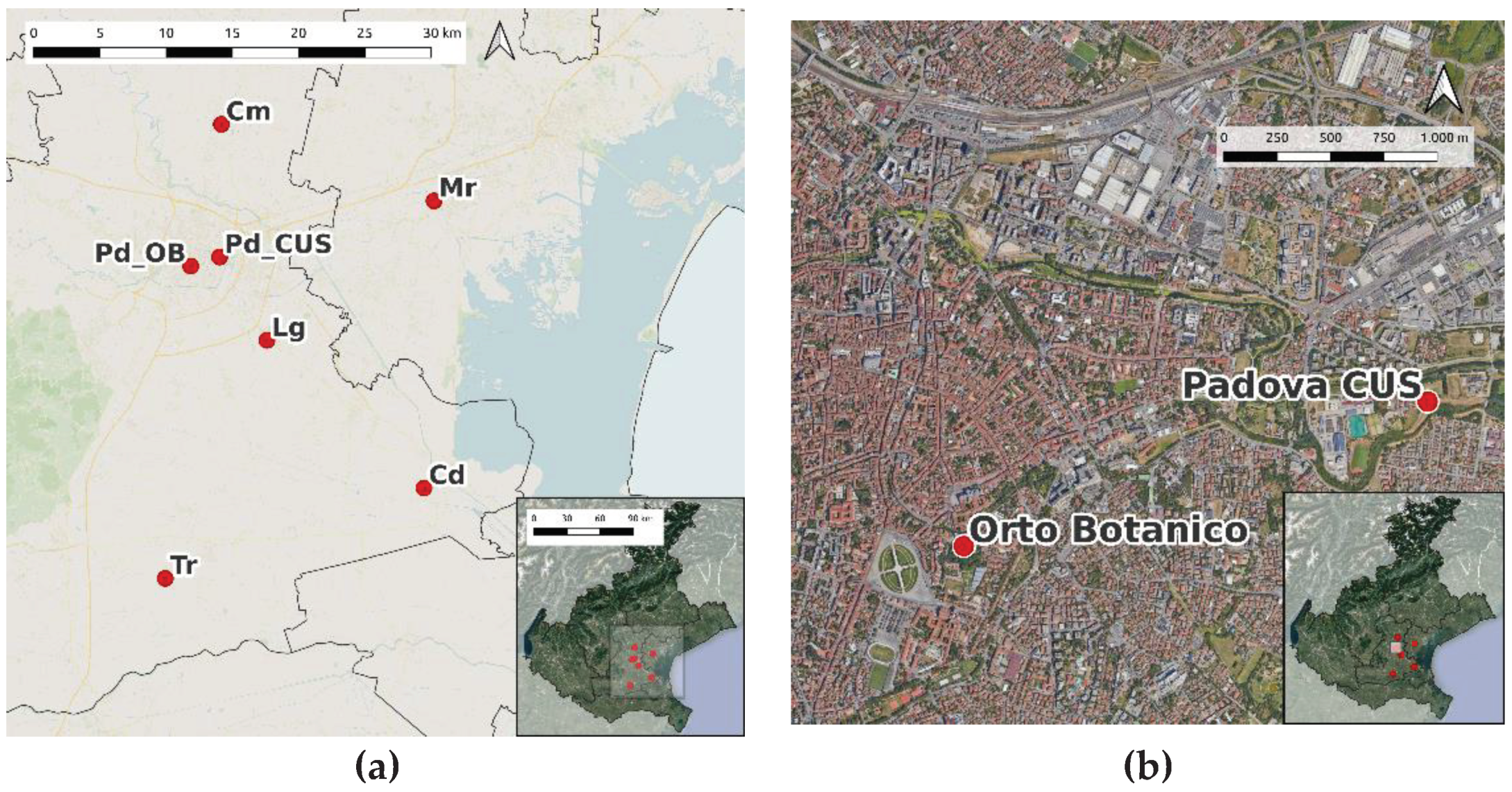
Figure 2.
Overlapping between the hours of observation of 9-9 series and the adjusted series, the latter composed of Fj=9 hours of the target day j in the 9-9 series, and Fj+1=15 hours of the day after (j+1) in the 9-9 series.
Figure 2.
Overlapping between the hours of observation of 9-9 series and the adjusted series, the latter composed of Fj=9 hours of the target day j in the 9-9 series, and Fj+1=15 hours of the day after (j+1) in the 9-9 series.

Figure 3.
Scatter plots of the 0-24 series of Padua compared to: (a) 9-9 series; 9-9 adjusted series (b) using 1day method; (c) using uniform method; (d) using ERA5 method; (e) using NOAA method; (f) Scatter plot of the monthly original Padua series compared to the adjusted series using the 4 methods.
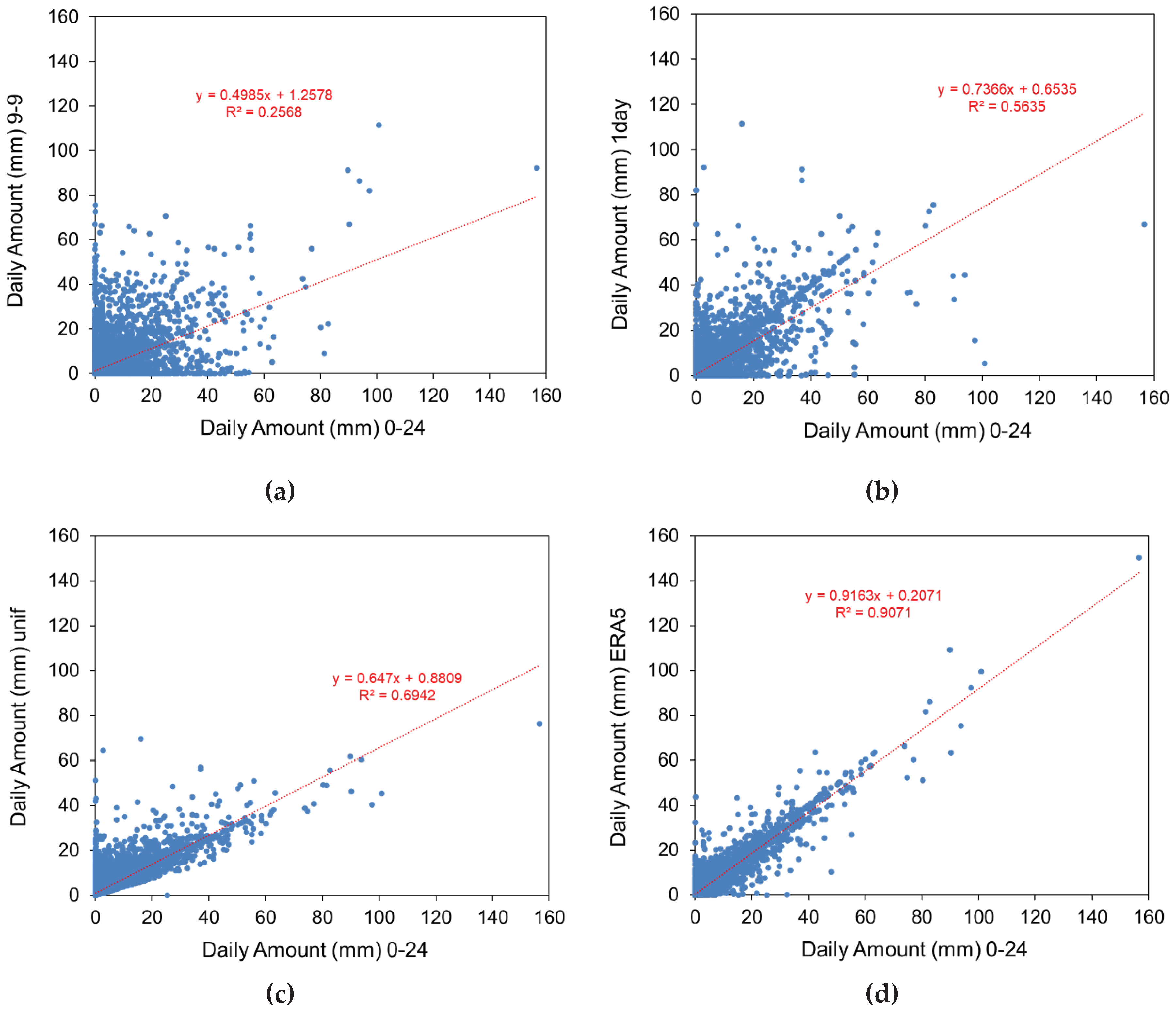
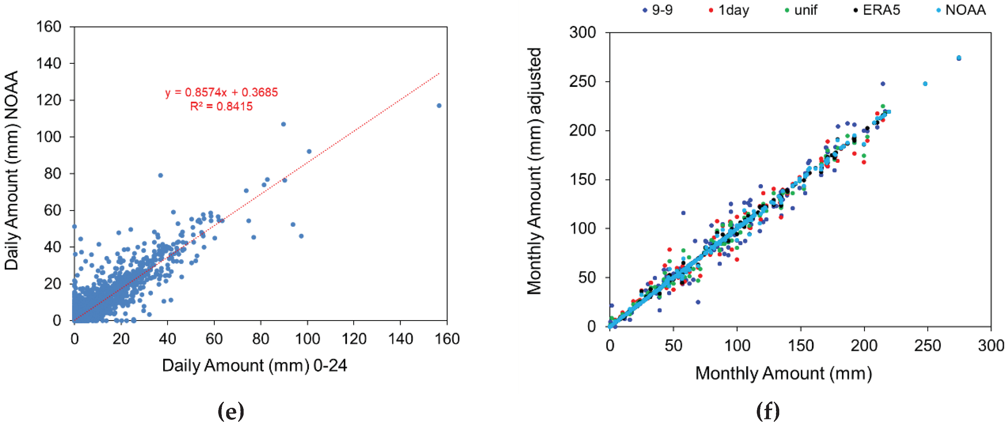
Figure 4.
Values of the indicators calculated for each adjustment method applied to each station. RMSE and MAE are expressed in mm, mwet and freq as percentage.
Figure 4.
Values of the indicators calculated for each adjustment method applied to each station. RMSE and MAE are expressed in mm, mwet and freq as percentage.
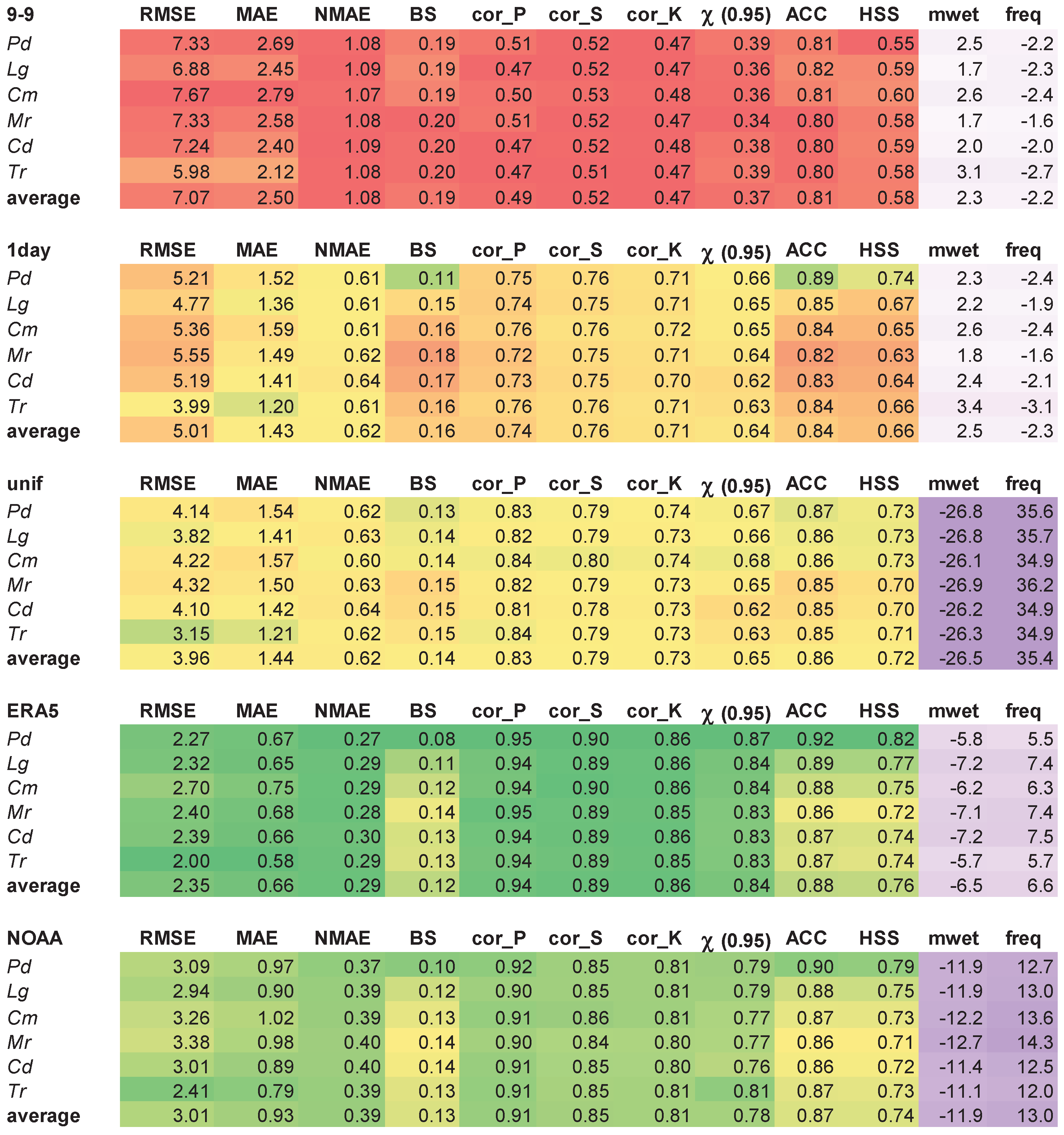
Figure 5.
Values averaged over all stations of precipitation (a) frequency; (b) mean value over wet days.
Figure 5.
Values averaged over all stations of precipitation (a) frequency; (b) mean value over wet days.
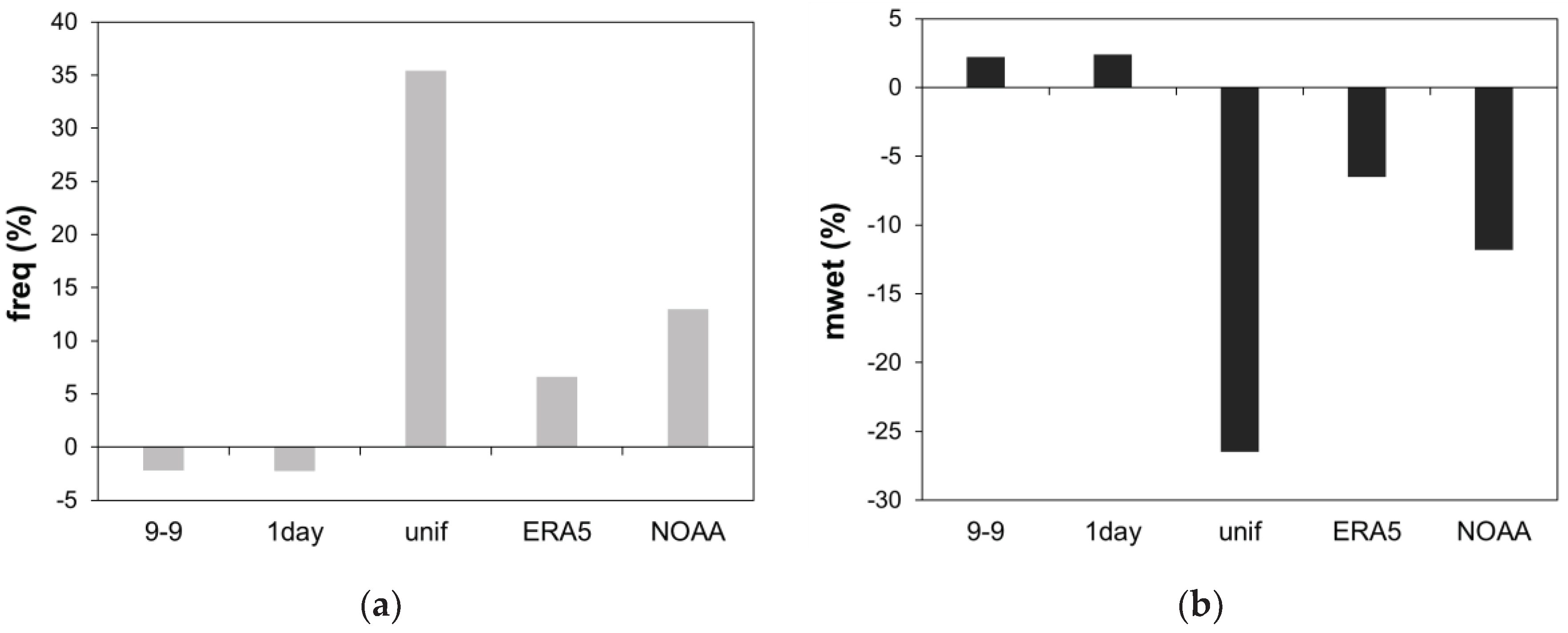
Figure 6.
Values of the indicators calculated for the adjusted Padua series compared to the 0-24 series of other stations. RMSE and MAE are expressed in mm.
Figure 6.
Values of the indicators calculated for the adjusted Padua series compared to the 0-24 series of other stations. RMSE and MAE are expressed in mm.

Figure 7.
Results of PCA applied to the dataset 10 (stations/methods) x 12 (indicators): (a) loading plot of PC1 vs PC2; (b) scores plot on PC1 vs PC2.
Figure 7.
Results of PCA applied to the dataset 10 (stations/methods) x 12 (indicators): (a) loading plot of PC1 vs PC2; (b) scores plot on PC1 vs PC2.
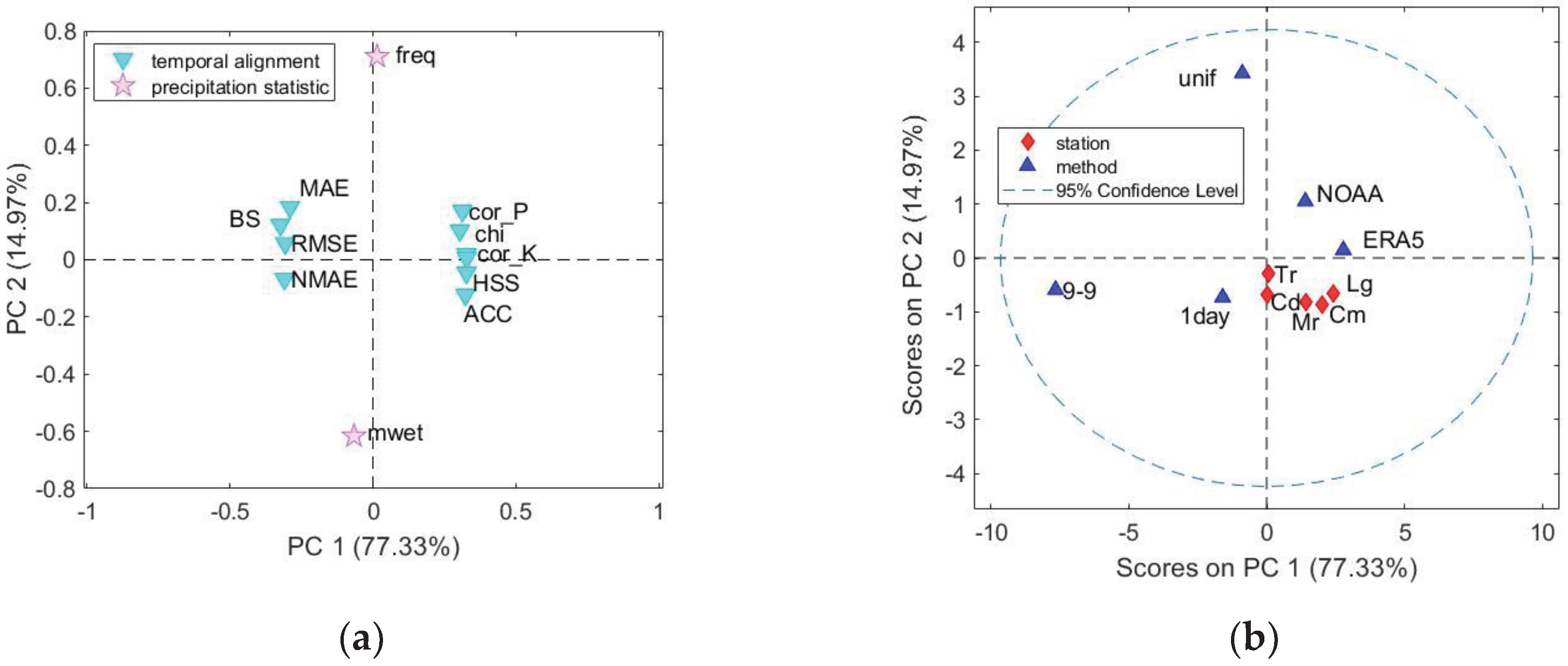
Figure 8.
3-way PARAFAC model of monthly values of performance indicators for Padua. Loadings on factor 1 of the three modes of data analysis: (a) Mode1-adjustment methods; (b) Mode2-performance indicators; (c) Mode3-month of the year.
Figure 8.
3-way PARAFAC model of monthly values of performance indicators for Padua. Loadings on factor 1 of the three modes of data analysis: (a) Mode1-adjustment methods; (b) Mode2-performance indicators; (c) Mode3-month of the year.
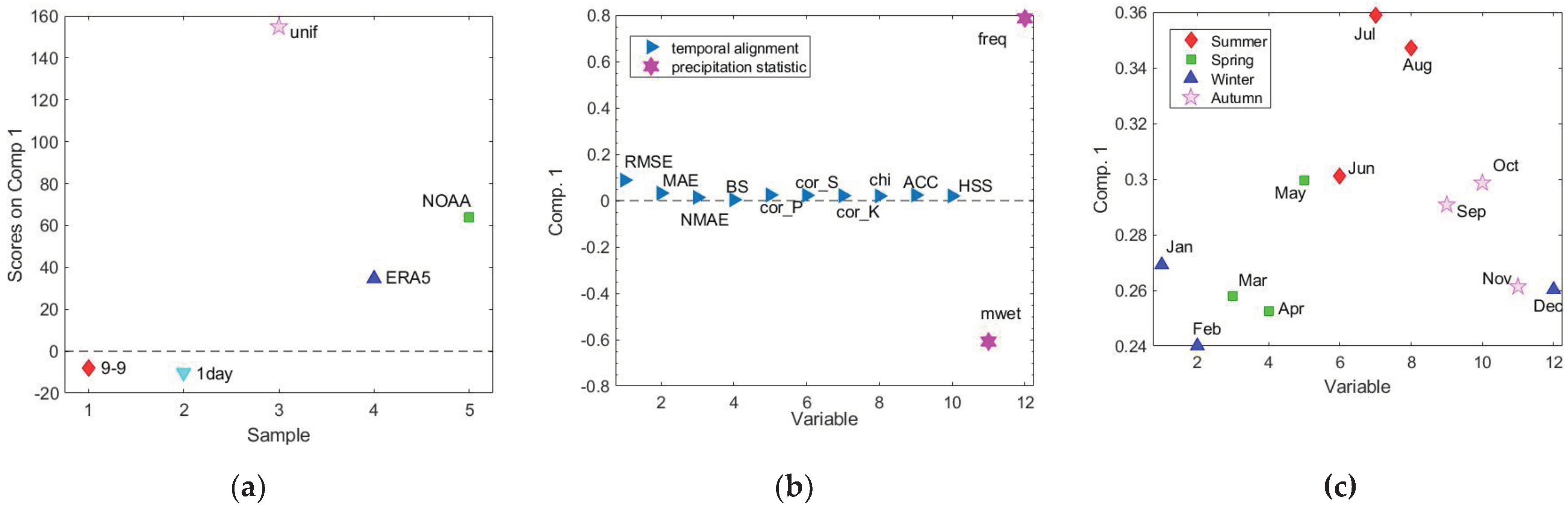
Figure 9.
3-way PARAFAC model of monthly values of performance indicators related to temporal alignment for Padua. Loadings on factor 1 of (a) Mode1-adjustment methods; (b) Mode2-performance indicators; (c) Mode3-month of the year.
Figure 9.
3-way PARAFAC model of monthly values of performance indicators related to temporal alignment for Padua. Loadings on factor 1 of (a) Mode1-adjustment methods; (b) Mode2-performance indicators; (c) Mode3-month of the year.
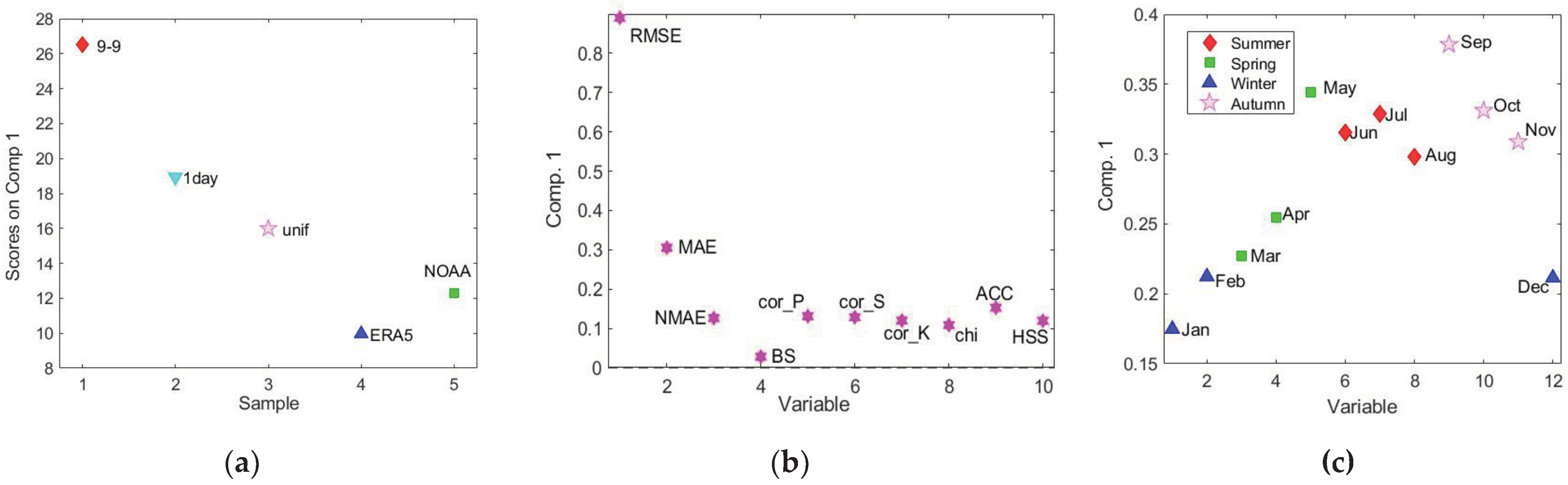
Figure 10.
Results of PCA applied to the dataset 60 (12 months x 5 methods) x 10 (indicators): (a) loading plot of PC1; scores plot on PC1 differentiating (b) the methods; (c) the seasons.
Figure 10.
Results of PCA applied to the dataset 60 (12 months x 5 methods) x 10 (indicators): (a) loading plot of PC1; scores plot on PC1 differentiating (b) the methods; (c) the seasons.
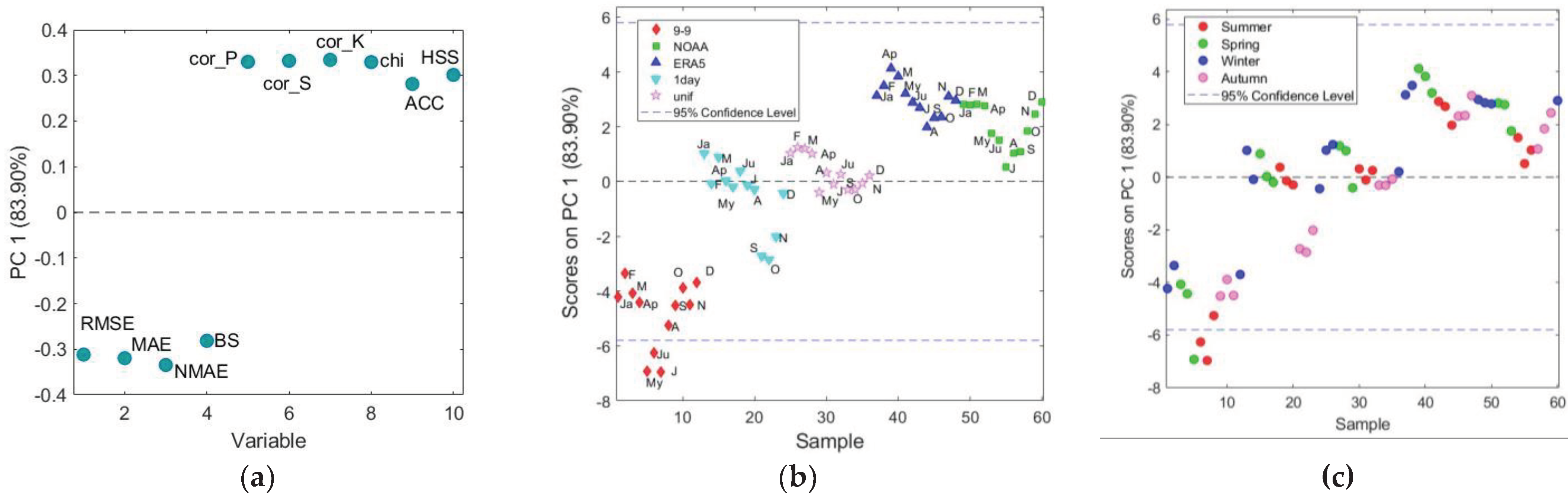
Figure 11.
Percentiles of the daily series: (a) values of the percentiles from the 50-ile to the 100-ile for the original and adjusted Padua series; (b) percentage difference between the percentile values from the 90-ile to the 100-ile of the adjusted Padua series and the neighboring series, and the 0-24 Padua series; (c) absolute values of the differences in (b).
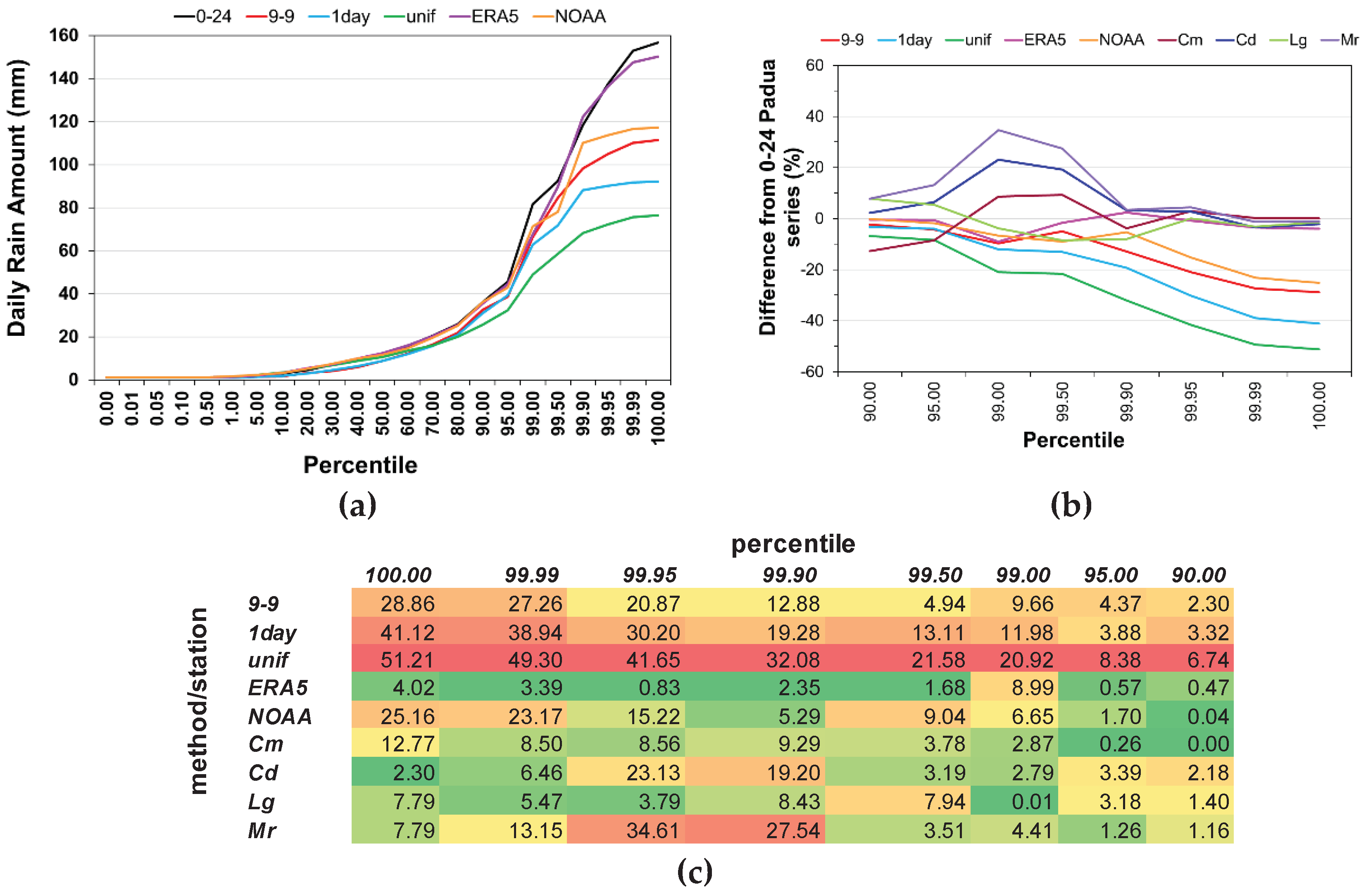
Figure 12.
Percentage difference respect to the 0-24 series of Padua of the precipitation amounts related to the 10, 20 and 30-year return periods for the different adjustment methods and the 0-24 series of Legnaro.
Figure 12.
Percentage difference respect to the 0-24 series of Padua of the precipitation amounts related to the 10, 20 and 30-year return periods for the different adjustment methods and the 0-24 series of Legnaro.
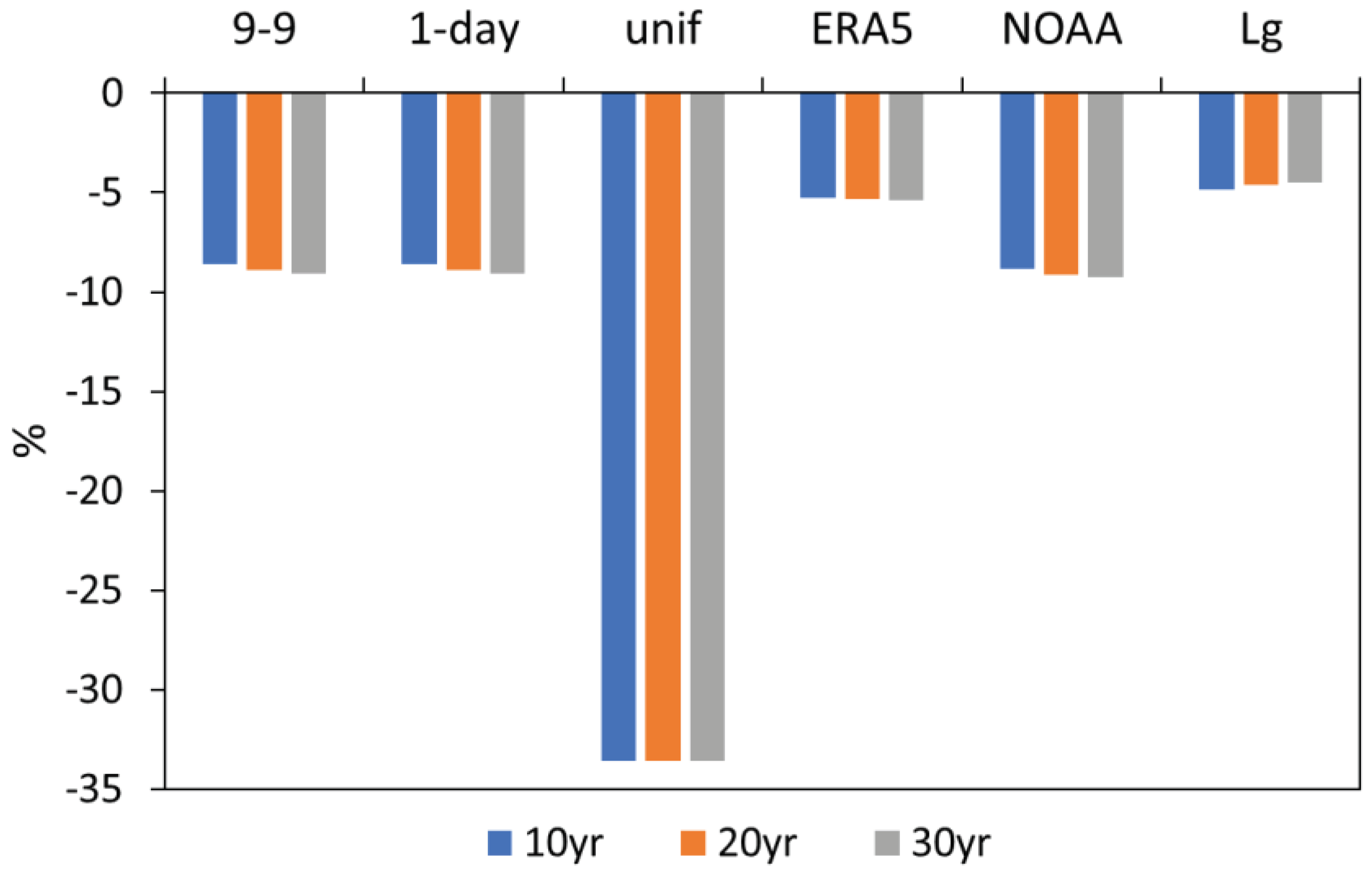

Table 1.
ARPAV meteorological stations in proximity of Padua, and data availability with respect to the 1993-2022 period.
Table 1.
ARPAV meteorological stations in proximity of Padua, and data availability with respect to the 1993-2022 period.
| Name | Acronym | Elevation (m a.g.l.) | Lat | Long | Distance from OB (km) | Data Availability |
|---|---|---|---|---|---|---|
| Orto Botanico | Pd | 12 | 45.39934 | 11.88049 | 0 | Oct 1993-Dec 2022 (97.1%) |
| Padova CUS | 12 | 45.40496 | 11.90848 | 2.3 | ||
| Legnaro | Lg | 7 | 45.34735 | 11.95217 | 8.0 | Jan 1993-Dec 2022 (99.5%) |
| Campodarsego | Cm | 16 | 45.49552 | 11.91336 | 11.0 | Jan 1993-Dec 2022 |
| (99.1%) | ||||||
| Codevigo | Cd | 0 | 45.24367 | 12.09971 | 24.4 | Jan 1993-Dec 2022 (99.4%) |
| Mira | Mr | 3 | 45.43935 | 12.11692 | 19.0 | Jan 1993-Dec 2022 (99.4%) |
| Tribano | Tr | 3 | 45.18669 | 11.84880 | 23.8 | Jan 1996-Dec 2022 (99.0%) |
Table 2.
Indicators used to evaluate the temporal alignment of the test and reference series.
| Name | Short Name |
|---|---|
| Root Mean Square Error | RMSE |
| (Normalized) Mean Absolute Error | (N)MAE |
| Brier Score | BS |
| Pearson correlation coefficient | cor_P |
| Spearman’s rank correlation | cor_S |
| Kendall’s rank correlation | cor_K |
| Tail dependence measure | χ(0.95) |
| Accuracy | ACC |
| Heidke Skill Score | HSS |
Table 3.
Indicators used to evaluate the precipitation statistics of the test and reference series.
| Name | Short Name |
|---|---|
| mean precipitation value over wet days | mwet |
| frequency of wet days | freq |
Table 4.
Significant parameters of the linear regression applied to original and adjusted Padua monthly series.
Table 4.
Significant parameters of the linear regression applied to original and adjusted Padua monthly series.
| Adjustment method | R2 | RMSE (mm) |
|---|---|---|
| 9-9 | 0.979 | 7.9 |
| 1day | 0.991 | 5.2 |
| unif | 0.994 | 4.2 |
| ERA5 | 0.998 | 2.3 |
| NOAA | 0.997 | 2.6 |
Disclaimer/Publisher’s Note: The statements, opinions and data contained in all publications are solely those of the individual author(s) and contributor(s) and not of MDPI and/or the editor(s). MDPI and/or the editor(s) disclaim responsibility for any injury to people or property resulting from any ideas, methods, instructions or products referred to in the content. |
© 2024 by the authors. Licensee MDPI, Basel, Switzerland. This article is an open access article distributed under the terms and conditions of the Creative Commons Attribution (CC BY) license (http://creativecommons.org/licenses/by/4.0/).
Copyright: This open access article is published under a Creative Commons CC BY 4.0 license, which permit the free download, distribution, and reuse, provided that the author and preprint are cited in any reuse.


